Dynamic Power Dispatch Considering Electric Vehicles and Wind Power Using Decomposition Based Multi-Objective Evolutionary Algorithm

Abstract

The intermittency of wind power and the large-scale integration of electric vehicles (EVs) bring new challenges to the reliability and economy of power system dispatching. In this paper, a novel multi-objective dynamic economic emission dispatch (DEED) model is proposed considering the EVs and uncertainties of wind power. The total fuel cost and pollutant emission are considered as the optimization objectives, and the vehicle to grid (V2G) power and the conventional generator output power are set as the decision variables. The stochastic wind power is derived by Weibull probability distribution function. Under the premise of meeting the system energy and user’s travel demand, the charging and discharging behavior of the EVs are dynamically managed. Moreover, we propose a two-step dynamic constraint processing strategy for decision variables based on penalty function, and, on this basis, the Multi-Objective Evolutionary Algorithm Based on Decomposition (MOEA/D) algorithm is improved. The proposed model and approach are verified by the 10-generator system. The results demonstrate that the proposed DEED model and the improved MOEA/D algorithm are effective and reasonable.

1. Introduction

Due to the serious deterioration of the global environment and the shortage of energy resources, protecting the environment and saving energy resources have become global concerns. Nowadays, most of the word’s power plants are consuming non-renewable energy such as coal and oil. Burning of fossil fuels, which exhaust gases, represent a major portion of global pollution emission. Therefore, reducing fuel costs and pollution emissions are an urgent problem that should be solved in power system.

Environment economic dispatch (EED) is a fundamental problem of power system dispatching, which aims at distributing available electric power generation to meet the load demand with the minimal possible fuel cost and pollution emission while satisfying all equality and inequality constraints in the power system [1]. In most studies, EED mainly focuses on optimizing the use of fossil fuels for convention generators, and model their work as a single objective function by linear combination of different objectives as a weighted sum [2,3]. Moreover, because of the environment damage caused by the burning of fossil fuels, renewable energy generation, such as wind power, is rapidly developing and getting the support of governments [4]. However, due to the randomness of wind speed, the output of wind power generation would be uncertain. The high penetration of wind power makes the EED problem significantly complicated. First, according to the U-shape emission function, adopting wind power will compensate for a part of the load demand and change the active power output of the thermal power units, but decreasing and increasing the wind power will not lead to the changes of the corresponding emission. Second, the stochastic fluctuation of wind power would also increase the operational risk of power system considering the power balance. Therefore, it is vital to reasonably model the uncertainty of wind power in the EED problem to ensure the effectiveness and rationality of the dispatch schemes.

In recent years, researchers have proposed many methods to deal with EED with wind power problems [5,6,7,8,9,10,11]. In [5], Ai et al. established the credibility distribution function model of wind power forecast errors. A fuzzy credibility index was presented to develop a fuzzy chance constrained model considering valve point effect for Dynamic Economic dispatch (DED) integrated wind farm. The chaotic particle swarm optimization was applied to optimize this model. Mondal et al. [6] employed the Price Penalty Factors (PPFs) to transform the multi-objective EED with wind power into one objective. Furthermore, a new optimization technique named Gravitational Search Algorithms (GSA) was applied. Yao et al. [7] proposed the Quantum-inspired Particle Swarm Optimization (QPSO) to solve the stochastic Economic Dispatch (ED) model involving wind power generation and carbon tax. The model of stochastic wind power is based on nonlinear wind power curve and Weibull distribution. In [8], Jiang et al. established a Wind-thermal Economic Emission Dispatch (WTEED) model, where the wind power cost was considered as a part of the optimization objective function. The cost of wind energy including overestimation and underestimation of available wind power was modeled by the Weibull-based probability densify function. The Gravitational Acceleration Enhanced Particle Swarm Optimization (GAEPSO) algorithm was applied to optimize the costs and emission objectives. In [9], Alham et al. proposed a multi-objective optimization model considering the wind power uncertainty. The multi-objective problem can be transformed into a single objective optimization problem by the weighted sum method, where the optimal Pareto front is obtained by changing weight factors. In [10], Zhu et al. described the stochastic of wind power application using the Weibull probability function, and established a multi-objective EED model. However, the influence of transmission losses on the dispatching system is still not considered. Finally, the rationality and feasibility of the model are verified by the improved evolutionary algorithm based on decomposition. In [11], Qu et al. applied the same processing method for wind power. In the established EED model, the constraint conditions, such as the transmission losses, the reserve capacity, etc. were considered. The Summation based Multi-Objective Differential Evolutionary (SMODE) algorithm was employed to optimize the EED problem and analyze the impact of wind power on power system.

The development of electric vehicles (EVs) is another new challenge to power system operation. Generally, EVs are completely or partly powered by electricity, which have significant advantages in reducing carbon emission, mitigating noise and improving energy efficiency over traditional cars. Governments have made series of policies to encourage the development of EVs. Studies demonstrate that, with the development of medium speed, electric vehicles’ market share in USA would reach 35% in 2020, 51% in 2030 and 62% in 2050 [12]. Due to the randomness of the charging behavior of EVs, it will bring great uncertainty to power system operation. On the other hand, EVs could also be used as energy storage devices. Study shows that most EVs are employed in only 4% of a day [13]. Furthermore, through Vehicle to Grid (V2G) technology, EVs can discharge to the power grid at the peak load and charge at low load from the power grid [14]. Therefore, EVs are an effective measure to relieve the intermittent of wind power by providing electricity. How to fully utilize the V2G function of EVs for power system service has been a hot topic in academia and industry [15,16,17,18,19,20,21,22,23,24,25].

Saber and Gholami et al. [15,16] established a single objective dispatch model by including economic and environmental factors, and the model was solved by the PSO algorithm. However, it only considered the registered EVs and the basic battery capacity rather than the user travel demand and the battery charging and discharging characteristics. In [17], Gan et al. pointed out that with an increased number of EVs and growing computational complexity, a decentralized approach could be potentially suitable. Zhao et al. [18] proposed an ED model, considering the uncertainties of EVs and wind power, and analyzed mathematical expectations of the generation costs of V2G power and wind power. An enhance Particle Swarm Optimization (PSO) was used to solve the ED model. Considering the user demand, Wu et al. [19] established three coordinated wind-EV energy dispatch models based on meeting the wind power efficiency and power load demands. In [20], Haque et al. proposed a model of Unit Commitment (UC) and Economic Dispatch (ED) based on an imbalance cost, which reflected the uncertainty of wind generation along with the marginal generation cost. The proposed UC-ED model utilized the flexibility of EVs to compensate the uncertainty wind power optimally. Many scholars established the model of EVs by considering either the power side demand or the user side demand [21,22,23,24,25]. However, few studies combine EVs with EED model for dispatch research, to realize dynamic management of EVs charging and discharging behavior.

The EED problem study is mostly focused on static dispatching. However, the above literature review shows that the dynamic economic emission dispatch (DEED) model is more suitable for the power system dispatching problem considering the EV and random wind power. At present, few works address the coordination dispatch of the wind power and EVs, especially, the DEED with wind power and EVs. In [26], Jiang et al. proposed a single objective dynamic optimization model, considering the coordination between EVs and renewable energy sources. However, the process of renewable energy such as wind power is not described in detail. In [27], Andervazh et al. presented a probabilistic optimization framework for the EED of thermal power generation units and considered the stochastic charging demand of EV and correlation wind power plants. Moreover, considering the uncertainty of wind power and EVs, the DEED model will become a high-dimension and multi-period form, which makes the problem more complex and a higher demand to the performance of the algorithms. Hence, the related work need to be further researched.

In this paper, a novel dynamic economic emission dispatch (DEED) model is developed by considering the EVs and uncertainties of wind power. The EVs power and the output power of thermal generator will be taken as the decision variables. The wind power will be treated as system constraints, including stochastic variables, and chance-constrained based programming method. Moreover, the power balance constraint, the user travel demand and on-board battery charging, discharging characteristics, etc., are included in the constraints. The total fuel cost and the total pollutant emission are set as the two optimization objectives. The MOEA/D algorithm which was proposed by Zhang et al. [28] in 2007 and has been successfully implemented in many fields [29,30,31], is applied to solve the proposed DEED model. At the same time, appropriate improvements are made to MOEA/D according to the characteristics of such a specific problem. The proposed DEED model and MOEA/D algorithm are tested by using a 10-generator system with EVs and wind farms, with the purpose of demonstrating the advantage of the proposed MOEA/D algorithm over other algorithms. The results demonstrate that proposed DEED model and MOEA/D algorithm are effective and reasonable.

The rest of the paper is organized as follows. Section 2 describes the modeling of the wind power and EVs. The modeling of DEED problem with EVs and wind power is presented in Section 3. In Section 4, the implementation of the algorithm and the constraints handing method are presented. The experiment setup, results and discussions are shown in Section 5. Section 6 concludes the paper.

2. Modeling of Wind Power and EVs

2.1. Modeling of Wind Power

The output power of the wind generator is determined by the change of wind speed, which has the typical stochastic and intermittent features. The study shows that the characteristic of wind speed can be modeled by a two-parameter Weibull probability distribution function [32]. The Cumulative Distribution Function (CDF) and Probability Destiny Function (PDF) of the wind speed can be written, respectively, as follow:

$$F(v)=1-\exp [-{(v/c)}^k],v\ge 0$$

(1)

$$f(v)=(k/c){(v/c)}^{k-1}\exp [-{(v/c)}^k],v\ge 0$$

(2)

where F(v) and f(v) are the CDF and PDF, respectively; v (m/s) is the wind speed; k is the shape factor; and c is the scale factor.

The relationship between the wind speed and output power of wind generator can be described as:

$$P_w=\{\begin{array}{ll}0,\hfill & v<v_{in}\mathrm{or}v\ge v_{out}\\ P_{rate}\frac{v-v_{in}}{v_{rate}-v_{in}},\hfill & v_{in}\le v<v_{rate}\\ P_{rate},\hfill & v_{rate}\le v<v_{out}\end{array}$$

(3)

where P_rate is the rated output wind power. v_rate, v_in and v_out are the rated cut-in and cut-out wind speed, respectively. As can be seen from Formula (3), P_w is a mixed random variable. In the interval (0, P_rate), P_w is continuous and the other intervals are discrete. The CDF of P_w in $\left(-\infty ,+\infty \right)$ is calculated as:

$$F(P_w)=\{\begin{array}{ll}0,\hfill & P_w<0\\ 1-\exp \{-{[(1+\frac{v_{rate}-v_{in}}{v_{in}{P}_{rate}}{P}_w)\frac{v_{in}}{c}]}^k\}+\exp [-{(\frac{v_{out}}{c})}^k],\hfill & 0\le P_w<P_{rate}\\ 1,\hfill & P_w\ge P_{rate}\end{array}$$

(4)

2.2. Modeling of Electric Vehicles

It is difficult to control a single EV, therefore, the model using the double-layer dispatch strategy is employed, i.e., the upper layer is the grid power dispatch center, the middle layer is the EVs agency, and the substratum is the user unit. The agency has a sub-regional management of EVs, and one region is an EVs cluster. First, the upper management sends the dispatch plan to the agency. Then, the agency management according to the actual situation assign the dispatch plan to the EVs cluster. As shown in Figure 1.

Since EVs are already registered in the power system, the owners have opted for their vehicles’ batteries to participate in V2G transactions. Assume that the number of EVs is N_v2g in the system and each of them has the same energy demand. The total EVs rated power in an interval of dispatch can be expressed as:

$$P_{v2g}={\displaystyle \sum _{i=1}^{N_{v2g}}{P}_{rv2g}}(i)$$

(5)

where P_rv2g (i) is rated power of the ith EV and P_v2g is the total EVs ratted power.

In each interval of dispatch, the EVs charging and discharging are not simultaneous, the states of which can be represented by the sign function (sgn) as follows:

$$\{\begin{array}{ll}{P}_{ch.t}=\mathrm{sgn}(x)P_{v2g},& x<0\\ P_{Dch.t}=\mathrm{sgn}(x)P_{v2g},& x>0\end{array}$$

(6)

where x < 0 and x > 0 denote the charge and discharge states, respectively. At x = 0, EVs do not participate in power system dispatch.

3. Modeling of DEED Problem with EVs and Wind Power

Many uncertain factors, such as the charging and discharging behavior of EVs, the wind power output, and the system load demand, are involved in the DEED problem. In this section, a DEED model is proposed to minimize the fuel cost and the pollution emission.

3.1. Objective Functions

Because EVs and wind farms participate in power system dispatch, the objective functions become dynamic compared with the classical EED problem.

Here, the total fuel cost objective can be defined as [33]:

$$\mathrm{Minimize}{F}_C={\displaystyle \sum _{t=1}^T{\displaystyle \sum _{i=1}^N(a_i+b_i{P}_{i.t}+c_i{P}_{i.t}^2)}}$$

(7)

where a_i, b_i, and c_i are the cost coefficients of ith power generator. T is the total dispatching period. P_i.t is output power of ith unit at time t. F_C is the total fuel cost of the system. N is the number of thermal generator units.

Furthermore, the total pollution emission objective can be defined as:

$$\mathrm{Minimize}{E}_M={\displaystyle \sum _{t=1}^T{\displaystyle \sum _{i=1}^N[({\alpha }_i+{\beta }_i{P}_{i.t}+{\gamma }_i{P}_{i.t}^2+{\zeta }_i\exp ({\phi }_i{P}_{i.t})]}}$$

(8)

where α_i, β_i, γ_i, ζ_i and ϕ_i are the emission coefficients of the ith power generator. E_M is the total pollution emission of the system.

3.2. System Constrain Conditions

Due to the presence of EVs charging and discharging power and wind power, which is different from the traditional environment economic dispatch, the system constraints are not deterministic but possess stochastic characteristics. The constraints are described in the form of probability, and the addition of stochastic variables makes the inequality constraints hold at a certain confidence level. The confidence level reflects the requirements of the power system operation.

3.2.1. Power Balance Constraint

The total output power of thermal generators, the output power of wind farms and EVs charging and discharging power must cover the total load demand and the transmission loss with certain confidence level.

$$P\left\{{\displaystyle \sum _{t=1}^N{P}_{i.t}}+P_{Dch.t}+P_w\ge P_{D.t}+P_{L.t}+P_{ch.t}\right\}\ge {\eta }_1$$

(9)

where P_ch.t and P_Dch.t are the EVs charging and discharging power in the time interval t. P_w is the active power output of wind farms. P_D.t is demanded power in the time interval t. ${\eta }_1$ is confidence level that represents the power system meets the load demand. It is generally selected to be close to 1 as value less than one means high operation risk. The other confidence levels in the following are similar to ${\eta }_1$. P_L.t is the transmission loss in the time interval t, which can be calculated by using the B-coefficients method [34].

$$P_{\mathrm{L}.\mathrm{t}}={\displaystyle \sum _{i=1}^N{\displaystyle \sum _{j=1}^N{P}_{i.t}{B}_{ij}}}{P}_{j.t}+{\displaystyle \sum _{i=1}^N{P}_{i.t}}{B}_{i0}+B_{00}$$

(10)

where B_i,j, B_i0 and B₀₀ are the network loss coefficients.

For chance-constrained programming problem a common method is to transfer the constraints into a deterministic form. Formula (9) can be modified as:

$$P\left\{P_w<P_{D.t}+P_{L.t}+P_{ch.t}-{\displaystyle \sum _{t=1}^N{P}_{i.t}}-P_{Dch.t}\right\}=F(P_{D.t}+P_{L.t}+P_{ch.t}-{\displaystyle \sum _{t=1}^N{P}_{i.t}}-P_{Dch.t})\le 1-{\eta }_1$$

(11)

The change of wind speed and direction determine the output power of wind farms. Assuming that the wind generators have the same speed and direction, the power balance inequality constraint by combining Formulas (4) and (11) can be described as follows:

$$P_{D.t}+P_{L.t}+P_{ch.t}-{\displaystyle \sum _{t=1}^N{P}_{i.t}}-P_{Dch.t}\le \frac{c{P}_{rate}}{v_{rate}-v_{in}}{\left|\ln [{\eta }_1+\exp (-\frac{v_{out}^k}{c^k})]\right|}^{1/k}-\frac{v_{in}{P}_{rate}}{v_{rate}-v_{in}}$$

(12)

3.2.2. Battery Remain Power Constrain

The EVs on-board battery remaining power S_t at time stage t is defined as follows:

$$S_t=S_{t-1}+{\lambda }_C{P}_{ch.t}\Delta t-\frac{1}{{\lambda }_D}{P}_{Dch.t}\Delta t-S_{Trip.t}$$

(13)

where λ_C and λ_D are the coefficients of the charging and discharging efficiencies, respectively. ∆t is the dispatch interval, and the value is 1 in this paper. S_Trip.t is the EVs consumption in the process of driving power, which can be calculated as follows:

$$S_{Trip.t}=\Delta SL$$

(14)

where ∆S is the average power consumption of unit distance and L is driving distance.

To ensure the safety of the operation and service lifespan of the battery, the remaining power S_t is constrained by minimum and maximum.

$$S_{\min }\le S_t\le S_{\max }$$

(15)

3.2.3. EVs Charging and Discharging Power Constraint

The charging and discharging power of the EVs is less than the rated power.

$$\{\begin{array}{l}{P}_{ch.t}\le P_{Nch}\\ P_{Dch.t}\le P_{NDch}\end{array}$$

(16)

where P_Nch and P_NDch are the charging and discharging rated power of the EVs, respectively.

3.2.4. User Travel Constraint

The basic function of EVs is to meet the user’s travel requirements. Suppose that a charging and discharging cycle is completed in dispatch period, the following formula should be satisfied.

$${\displaystyle \sum _{t=1}^T{S}_{Trip.t}}={\displaystyle \sum _{t=1}^T{\lambda }_C{P}_{ch.t}\Delta t}-{\displaystyle \sum _{t=1}^T\frac{1}{{\lambda }_D}{P}_{Dch.t}\Delta t}$$

(17)

3.2.5. Ramp Rate Limits

Since the power output cannot change significantly between two adjacent intervals, the generators’ power ramp rates are limited.

$$\{\begin{array}{l}{P}_{i.t}-P_{i.t-1}-U_{Rt}\Delta t\le 0\\ P_{i.t-1}-P_{i.t}-D_{Rt}\Delta t\le 0\end{array}$$

(18)

where U_Rt and D_Rt are the ramp-up and ramp-down rate limits of the ith power generator, respectively.

3.2.6. Reserve Capacity Constraint

To reduce the impact of stochastic wind power and EVs charging and discharging power for the system, the up and down spinning reserves must to be considered.

The up spinning reserve constrain can be represented as follows:

$$P\left\{[{\displaystyle \sum _{i=1}^N(P_{i.t}^{\max }-P_{i.t})+}{P}_{Dch.t}]\ge {\omega }_u{P}_w+P_{ch.t}+S_{R.t}\right\}\ge {\eta }_2$$

(19)

Likewise, the down spinning reserve constrain can be represented as follows:

$$P\left\{[{\displaystyle \sum _{i=1}^N(P_{i.t}-P_{i.t}^{\min })+}{P}_{Dch.t}]\ge {\omega }_d(P_{rate}-P_w)+P_{ch.t}\right\}\ge {\eta }_3$$

(20)

where $P_{i.t}^{\max }$ and $P_{i.t}^{\mathrm{m}\mathrm{in}}$ are the maximum and minimum power of the ith generator in the time interval t. ω_u and ω_d are the demand coefficients of wind farm output on up and down spinning reserve. ${\eta }_2$ and ${\eta }_3$ are the confidence level. P_rate is the rated output of the wind farm. S_R.t is spinning reserve capacity requirements in the time interval t.

Similar to the power balance constraint, Formulas (19) and (20) could also be transformed into deterministic inequality constraints. The formula after transformation are written as follows:

$$\frac{1}{{\omega }_u}[{\displaystyle \sum _{i=1}^N(P_{i.t}^{\max }-P_{i.t})+}{P}_{Dch.t}]\ge \frac{c{P}_{rate}}{v_{rate}-v_{in}}{\left|\ln [1-{\eta }_2+\exp (-\frac{v_{out}^k}{c^k})]\right|}^{1/k}-\frac{v_{in}{P}_{rate}}{v_{rate}-v_{in}}$$

(21)

$$P_{rate}-\frac{1}{{\omega }_d}[{\displaystyle \sum _{i=1}^N(P_{i.t}^{\max }-P_{i.t})+}{P}_{Dch.t}]\le \frac{c{P}_{rate}}{v_{rate}-v_{in}}{\left|\ln [{\eta }_3+\exp (-\frac{v_{out}^k}{c^k})]\right|}^{1/k}-\frac{v_{in}{P}_{rate}}{v_{rate}-v_{in}}$$

(22)

3.2.7. Output Power Constraint

The power generators output constrain is shown as follows:

$$P_{i.t}^{\min }\le P_{i.t}\le P_{i.t}^{\max }$$

(23)

The wind farm output constraint could be represented as follows:

$$0\le P_w\le P_{rate}$$

(24)

3.3. Problem Formulation

Based on the above objectives and constraints, the DEED problem with EVs and wind power could be mathematically formulated as a nonlinear constrained multi-objective optimization problem as follows:

$$\{\begin{array}{lll}\mathrm{Minimize}\hfill & [F_C,E_M]\hfill & \\ \mathrm{subject}\mathrm{to}:\hfill & h_i(P_G)\le 0,\hfill & i=1,2,\dots ,I\\ \hfill & g_j(P_G)=0,\hfill & j=1,2,\dots ,J\\ \hfill & P_{G\min }\le P_G\le P_{G\max },\hfill & k=1,2,\dots ,n\end{array}$$

(25)

where P_G is the n dimensional decision variables to be optimized, and, in this, the decision variables include output power of thermal generator units and V2G power. h_i(P_G) and g_j(P_G) are inequality and equality constraints, respectively.

The best emission and cost are non-commensurable and competing in nature, i.e., no objective function can be best, and each advantages the other at the same time. Hence, with conflicting objective functions, multi-objective optimization gives rise to a set of optimal solutions instead of one optimal solution. These optimal solutions set are known as Pareto optimal solutions (PSs), which constitute the Pareto optimal Front (PF) in the entire search space. The aim of multi-objective problems is to find the PSs as much as possible and make them evenly distributed on PF.

Figure 2 shows the PF of a typical multi-objective problem. The extreme solution x₁ gives the maximum objective 2 and minimum objective 1, while the extreme solution x₅ provides the maximum objective 1 and minimum objective 2 among all the solutions PF, respectively. Hence, the extreme solutions x₁ or x₅ focus on optimizing one of the objective [10]. The decision makers can make choices (e.g., x₂, x₃ and x₄ in Figure 2) based on the tradeoff between the objectives 1 and 2.

4. The Implementation of MOEA/D

MOEA/D provides a new method by decomposition approaches for multi-objective optimization. It solves the problem of approximating the PF by decomposing a multi-objective problem into a number of scalar optimization subproblems, which are optimized concurrently.

4.1. Decompose Approach

There are several decomposition approaches for converting a multi-objective problem into a number of scalar subproblems [28]. However, the weighted Tchebyceff approach is less sensitive to the shape of PF among these decomposition approaches, which can be used to find the PSs in both convex and nonconvex PFs. In this paper, this approach is also adopted and can be formulated as follows:

$$\{\begin{array}{ll}\mathrm{Minimize}\hfill & g^{te}(x|\lambda ,z^{\ast })=\underset{1\le i\le m}{\max }\{{\lambda }_i\left|f_i(x)-z_i^{\ast }\right|\}\hfill \\ \mathrm{subject}\mathrm{to}\hfill & x\in S\hfill \end{array}$$

(26)

where S is the feasible space, $z^{\ast }={(z_1^{\ast },\dots ,z_m^{\ast })}^T$ is the reference point, m is the number of objective function and λ = (λ₁ … λ_m)^T is the weight vector. For each i = 1, …, m, there should be as:

$$\{\begin{array}{l}{z}_i^{\ast }=\min \{f_i(x)|x\in S\}\hfill \\ {\displaystyle \sum _{i=1}^m\lambda =1}\hfill \end{array}$$

(27)

Note that g^te is continuous of λ; if λⁱ and λ^j are close to each other, then the corresponding optimal solution of g^te(x|λⁱ, z*) should be close to g^te(x|λ^j, z*). Here, ${\lambda }^i,{\lambda }^j\in \left({\lambda }^1,\dots ,{\lambda }^N\right),\left({\lambda }^1,\dots ,{\lambda }^N\right)$ is a set of even spread weight vectors of N subproblems. Therefore, any information about these g^tes with weight vectors close to λⁱ should be helpful for optimization, which is defined as a neighborhood of weight vector λⁱ hereinafter. Only the current solutions to its neighboring subproblems are exploited for optimizing a subproblem in MOEA/D.

4.2. Constraints Handing Method

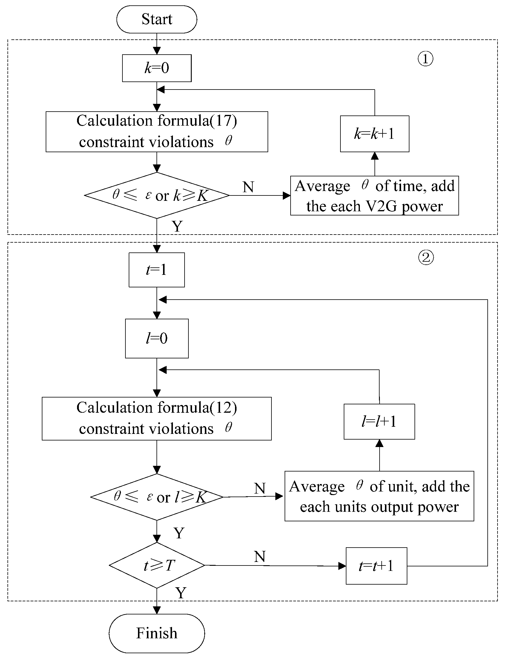
The key of the optimization model for DEED problem is how to solve the constraints condition, which is nonlinear, large-scale, high-dimension, non-convex and multi-period. In this paper, we propose a two-step strategy for dynamic adjustment of decision variables based on the penalty function.

(1)

The proposed model needs to meet the user travel demand equality constraints, according to Formula (17), to adjust the different time intervals of V2G power dynamically to meet the power balance of EVs.

(2)

Based on the V2G power and wind output power that have been obtained, adjust the thermal generator units output power in each time intervals by Formula (12), to ensure the system power balance.

The flow chart of the proposed two-step strategy is shown as Figure 3.

The above two-step process is described in detail as follows:

Step 1.

For Formulas (12) and (17), calculate their constraint violations (θ), respectively. If θ ≤ ε (threshold value), adjust the number of times k and l to reach the maximum value K then go to Step 3. Otherwise, go to Step 2.

Step 2.

According to the adjusted decision variables, θ/n (n is the time intervals or generator units number) is added to each decision variables. Perform the cross boundary processing according to the upper and lower output power limits of the variables.

Step 3.

If charging and discharging power adjustment to the demand of users, stop adjustment. If the generator unit output power balance is being adjusted, wait for all the time interval adjustments to be completed, and then stop.

In this paper, for other constraints in DEED model, the following classification method is used:

(1)

The EV charging and discharging power constraints, the output of generator unit’s constraints, and the ramp rate limit constraint are added to the cross-boundary processing of the dynamic adjustments.

(2)

Infeasible solutions after two-step processing, constraint violation of these solutions, battery remaining power constraint violation and spinning reserve constraint violation are set as the total of constraint violations V(x). In this paper, we adopt the following penalty function approach, which is simple but efficient: F(x) = f(x) + sV(x), where f(x) is one of the objective functions, s is the penalty coefficient, and V(x) can be defining as:

$$V(\mathit{x})=\left|{\displaystyle \sum _{i=1}^I\max (h_i(\mathit{x}),0)}\right|$$

(28)

Clearly, if V(x) = 0 the solutions are feasible. Otherwise, the solutions are infeasible.

4.3. Procedures of MOEA/D for DEED

Step 1.

(1)

Specify parameters of wind farms such as wind speed, active power limits and confidence level.

(2)

Specify parameters of each generator unit and EVs charging and discharging lower demand and active power limits, the cost and emission coefficients.

(3)

Set MOEA/D parameters such as the number of the weight vectors in the neighborhood of each weight vector (D) and population N_p.

(4)

Set the maximum number of generations, gen_max.

Step 2. Initialization

(1)

The decision variables of this DEED problem are generator active power outputs and the EVs charging and discharging power in each time intervals, which constitute the population x that can be expressed as: $\mathit{x}={\left[\begin{array}{cccc}{\mathit{x}}^1& {\mathit{x}}^2& \dots & {\mathit{x}}^{N_p}\end{array}\right]}^T$.

One of the dispatch schemes in the individual xⁱ can be represented as:

$${\mathit{x}}^i=\left\{\begin{array}{cccc}{P}_{1,1}& P_{1,2}& \dots & P_{1,T}\\ P_{2,1}& P_{2,2}& \dots & P_{2,T}\\ ⋮& ⋮& ⋮& ⋮\\ P_{N,1}& P_{N,2}& \dots & P_{N,T}\\ P_{ev,t}& P_{ev,t}& \dots & P_{ev,t}\end{array}\right\}$$

(29)

where P_ev.t is the charging or discharging power at time interval t. The dimensions of each individual is (N + 1) × T. When the EVs is charging, P_ev.t = P_ch.t, and, when discharging, P_ev.t = P_Dch.t.

(2)

For the each individual xⁱ, the objective function FVⁱ = F(xⁱ) = [F₁(xⁱ), F₂(xⁱ)]^T is calculated by the above constraints handing method. F₁(xⁱ) and F₂(xⁱ) are the cost and emission. Initialize the reference point z = [z₁, z₂]^T by setting $z_j=\underset{j=1,2,\dots ,N_p}{\min }[F_1(x^i),F_2(x^i)]$.

(3)

Initialize the weight vectors $\left({\lambda }^1,\dots ,{\lambda }^{N_p}\right)$, whose values are derived from $\left(\frac{0}{N_p-1},\frac{1}{N_p-1},\dots ,\frac{N_p-1}{N_p-1}\right)$ for two objectives. Choose the closest weight vectors to each weight vector based on the computed Euclidean distances between any two weight vectors. For each i = 1, ..., N_p, set B(i) = {i₁, ..., i_D}, and ${\lambda }^{i_1},\dots ,{\lambda }^{i_D}$ are the D closest weight vectors to ${\lambda }^i$.

(4)

Set the number of generations, and make gen = 0.

Step 3. Update

For i = 1, …, N_p, perform the following.

(1) Reproduction

Randomly select three indexes r₁, r₂ and r₃ from B(i), such that r₁ ≠ r₂ ≠ r₃ ≠ i. Then, generate a new solution y from $x^{r_1},x^{r_2}$ and $x^{r_3}$ by a DE operator according to the following formula as:

$$y=\{\begin{array}{ll}{x}^{r_1}+F\times (x^{r_2}-x^{r_3}),\hfill & CR\hfill \\ x^i,\hfill & 1-CR\hfill \end{array}$$

(30)

where F and CR are two control parameters.

To increase the diversity of population, generate a new solution y′ from y by a mutation operator with the probability of p_m as follow.

$$y^{\prime }=\{\begin{array}{ll}y+\sigma \times (u-l),\hfill & p_m\hfill \\ y,\hfill & 1-p_m\hfill \end{array}$$

(31)

with

$$\sigma =\{\begin{array}{ll}{(2\times rand)}^{\frac{1}{\eta +1}}-1,\hfill & rand<0.5\hfill \\ 1-{(2-2\times rand)}^{\frac{1}{\eta +1}},\hfill & \mathrm{otherwise}\hfill \end{array}$$

(32)

where u and l are the upper and lower bounds of decision variable, respectively. η is the distribution index.

(2) Repair

If any element of y′ is out of the boundary, reset it to be the boundary value.

(3) Update z

For each j = 1 or 2, if z_j < F_j(y′), set z_j = F_j(y′).

(4) Update the neighboring solutions

As shown in Equation (26), $g^{te}(y^{\prime }|\lambda ,z)=\underset{1\le i\le m}{\max }\{{\lambda }_i\left|F_i(y^{\prime })-z\right|\}$, including the penalty function. For each $j\in B(i)$, if $g^{te}(x^j|{\lambda }^j,z)\ge g^{te}(y^{\prime }|{\lambda }^j,z)$, then set x^j = y′, FV^j = F(y′).

Step 4. Stopping criteria

If gen = gen_max, then stop. Otherwise, set gen = gen + 1, and go to Step 3.

4.4. Best Compromise Solution

The results of the proposed MOEA/D optimization are called the PSs, which can provide one solution as the best compromise solution for the decision makers by a fuzzy-based method. Because of the imprecise nature of decision makers’ judgment, the ith objective function value of a solution in the Pareto-optimal set F_i is represented by membership function defined as [35]:

$${\mu }_i=\{\begin{array}{ll}1,\hfill & F_i\le F_i^{\min }\hfill \\ \frac{F_i^{\max }-F_i}{F_i^{\max }-F_i^{\min }},\hfill & F_i^{\min }\le F\le F_i^{\max }\hfill \\ 0,\hfill & F_i\ge F_i^{\max }\hfill \end{array}$$

(33)

where $F_i^{\min }$ and $F_i^{\mathrm{m}\mathrm{ax}}$ are the minimum and the maximum values of ith objective function, respectively.

For each non-dominated solution k, the normalized membership function values μ^k can be expressed as follow:

$${\mu }^k=\frac{{\displaystyle {\sum }_{i=1}^m{\mu }_i{}^k}}{{\displaystyle {\sum }_{k=1}^{N_{PF}}{\displaystyle {\sum }_{i=1}^m{\mu }_i{}^k}}}$$

(34)

where m is the number of objective functions, here m = 2; and N_PF is the number of non-dominated solutions, i.e., the number of solutions in PF. When μ^k is the maximum value, the corresponding solution is the best compromise solution. Then, all of the solutions are in a descending order according to their membership function, and, in view of the current operating conditions, the decision makers can be guided to get the tradeoff relations between cost and emission.

5. Experiment Result and Discussion

A 10-unit system with registered EVs and one wind power farm is selected in this section. The dispatch period is one day which is divided into 24 intervals. Load demand and unit characteristics of the 10-unit are obtained from [36,37] and can be found in

Table 1. Load demands for 24 h (10-unit system).

Hour	PD/MW	Hour	PD/MW	Hour	PD/MW	Hour	PD/MW
1	1036	7	1702	13	2072	19	1776
2	1110	8	1776	14	1924	20	1972
3	1258	9	1924	15	1776	21	1924
4	1406	10	2022	16	1554	22	1628
5	1480	11	2106	17	1480	23	1332
6	1628	12	2150	18	1628	24	1184

and

Table 2. Generator characteristics.

Unit	${\mathit{P}}_{\mathit{i}}^{\mathbf{min}}$	${\mathit{P}}_{\mathit{i}}^{\mathbf{max}}$	UR	DR	ai	bi	ci	αi	βi	γi	ζi	ϕi
	MW		MW/h		$/h	$/MWh	$/(MW)2h	lb/h	lb/MWh	lb/(MW)2h	lb/h	1/MW
P1	150	470	80	80	786.7988	38.5379	0.1524	103.3908	−2.4444	0.0312	0.5035	0.0207
P2	135	470	80	80	451.3251	46.1591	0.1058	103.3908	−2.4444	0.0312	0.5035	0.0207
P3	73	340	80	80	1049.9977	40.3965	0.0280	300.391	−4.0695	0.0509	0.4968	0.0202
P4	60	300	50	50	1243.5311	38.3055	0.0354	300.391	−4.0695	0.0509	0.4968	0.0202
P5	73	243	50	50	1658.5696	36.3278	0.0211	320.0006	−3.8132	0.0344	0.4972	0.0200
P6	57	160	50	50	1356.6592	38.2704	0.0179	320.0006	−3.8132	0.0344	0.4972	0.0200
P7	20	130	30	30	1450.7045	36.5104	0.0121	330.0056	−3.9023	0.0465	0.5163	0.0214
P8	47	120	30	30	1450.7045	36.5104	0.0121	330.0056	−3.9023	0.0465	0.5163	0.0214
P9	20	80	30	30	1455.6056	39.5804	0.1090	350.0056	−3.9524	0.0465	0.5475	0.0234
P10	10	55	30	30	1469.4026	40.5407	0.1295	360.0012	−3.9864	0.0470	0.5475	0.0234

. To demonstrate the effectiveness of the proposed method and model, four different cases are considered as follows:

Case 1:

The feasibility of the proposed DEED model and the validity of the proposed MOEA/D are verified in this case.

Case 2:

The influence of the different number of EVs on the power system, and the impact of EVs on environmental and economic under different permeability are studied.

Case 3:

The influence of wind power output on power system in DEED model is analyzed under three different parameters of wind power, i.e., confidence level η₁, shape factors k and scale factors c.

Case 4:

The interaction between EVs and wind power and the influence of different EVs and wind power on the power system are analyzed.

MATLAB R2014b is used as the simulation platform for comparing all the algorithms and the simulation are executed on a computer with Core I7-4790 CPU, 16 GB RAM and windows 10 64-bit operating system. The population sizes are set to 100 for all algorithms, and the maximum number of generations is set as 5000, except for the special instructions. Penalty coefficients are set to 100. Parameters set of proposed MOEA/D as follow: F = 0.6, CR = 0.9 and the distribution index η = 20, ε and K are selected as 10⁻⁶ and 10, respectively. The neighborhood D is selected as 20 and the mutation rate is selected p_m = 1/[(N + 1) × T].

5.1. Case 1

The purpose of this case is to verify the rationality of the proposed DEED model and MOEA/D. The battery capacity is 24 kWh and power consumption is 15 kWh/100 km. Suppose that the state of charge (SOC) of an EV every morning is 100%. Commuting occurs on roads (total 50 km) during 07:00–08:00 and 17:00–18:00, and the rest of the time the car participates in power grid dispatch. In dispatch cycle, minimum SOC and the rated power of charging and discharging are limited to 20% of the rated power, on-board battery charging and discharging power efficiency is 0.85, and the system’s spinning reserve demand is set as the load value of 10%.

To validate the proposed MOEA/D, other existing algorithms are compared to the proposed one, in the same test case. The other experimental parameters are set as follows. In MOPSO, the personal and global learning coefficients were selected as 2.05, the inertia weight coefficient was 0.729 [38]. In MODE, the scaling factor and crossover constant were set as 0.5 and 0.1, respectively, and the DE/rand/1 strategy was used [39]. In SPEA2, the crossover and mutation probabilities were chosen as 0.7 and 0.3, respectively [36]. In NSGA-II, the crossover and mutation probabilities were selected as 0.9 and 0.2, respectively [40]. Total number of wind turbines of a wind farm was 20, each turbine’s rating was 1.5 MW, and total rated output of wind farm was 30 MW. The v_in, v_rate and v_out were 5 m/s, 15 m/s and 45 m/s, respectively. The w_u and w_d were selected as 0.2 and 0.3, respectively. The confidence levels of ${\eta }_1$, ${\eta }_2$ and ${\eta }_3$ were selected as 0.5, 0.9 and 0.9. The shape factor k and scale factor c were set as 2.2 and 15 m/s, respectively.

All algorithms were run 30 times independently and the solutions were recorded. As shown in

Table 3. The solutions and average computation time (seconds) of different methods. (Cost (×10⁶) and Emission (×10⁵)).

Methods	MOEA/D		MODE		MOPSO		SPEA2
	Cost	Emission	Cost	Emission	Cost	Emission	Cost	Emission
Best cost	2.4238	2.9917	2.5447	2.9930	2.4304	3.0426	2.4481	3.0072
Best emission	2.5090	2.8175	2.5739	2.9460	2.4960	2.8965	2.4875	3.0057
Best compromise	2.4564	2.8652	2.5429	2.9722	2.4576	2.9648	2.4878	3.0063
Average time	3366.01		6582.86		5791.785		6737.04

, the best cost solutions obtained by MOEA/D, with reductions of $0.1209 × 10⁶, $0.0066 × 10⁶ and %0.0637 × 10⁶ compared to MODE, MOPSO and SPEA2, respectively. The best emission solutions obtained by MODE, MOPSO and SPEA2, increasing emissions by 0.1465 × 10⁵ lb, 0.0790 × 10⁵ lb and 0.1882 × 10⁵ lb compared with MOEA/D, respectively. The compromise solution obtained by MOEA/D is less than other algorithms. 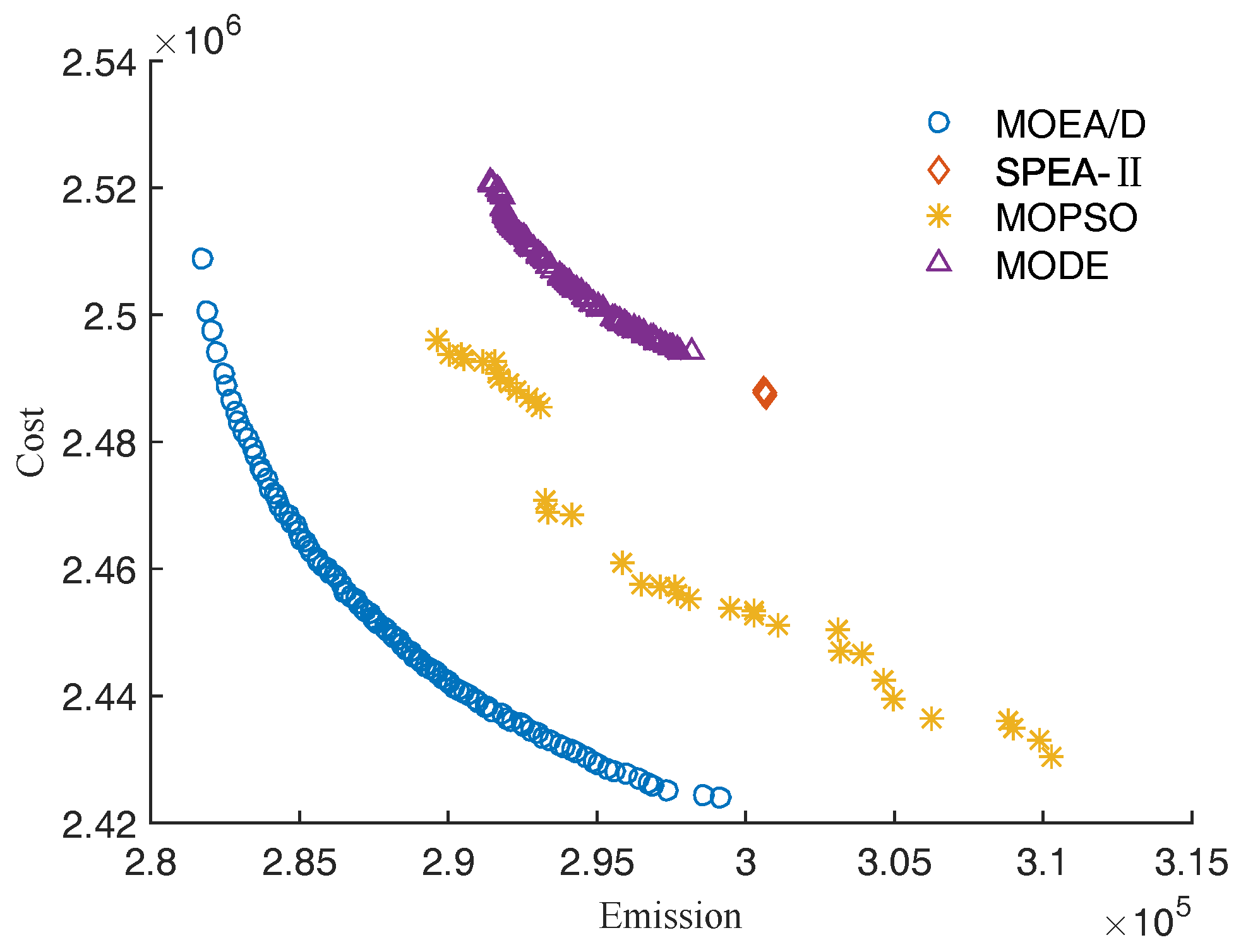The fuel cost and emission increased by a minimum of $0.0012 × 10⁶ and 0.0096 × 10⁵ lb, respectively. All the PFs obtained by corresponding methods are shown in Figure 4, in which MOEA/D is compared with other methods.

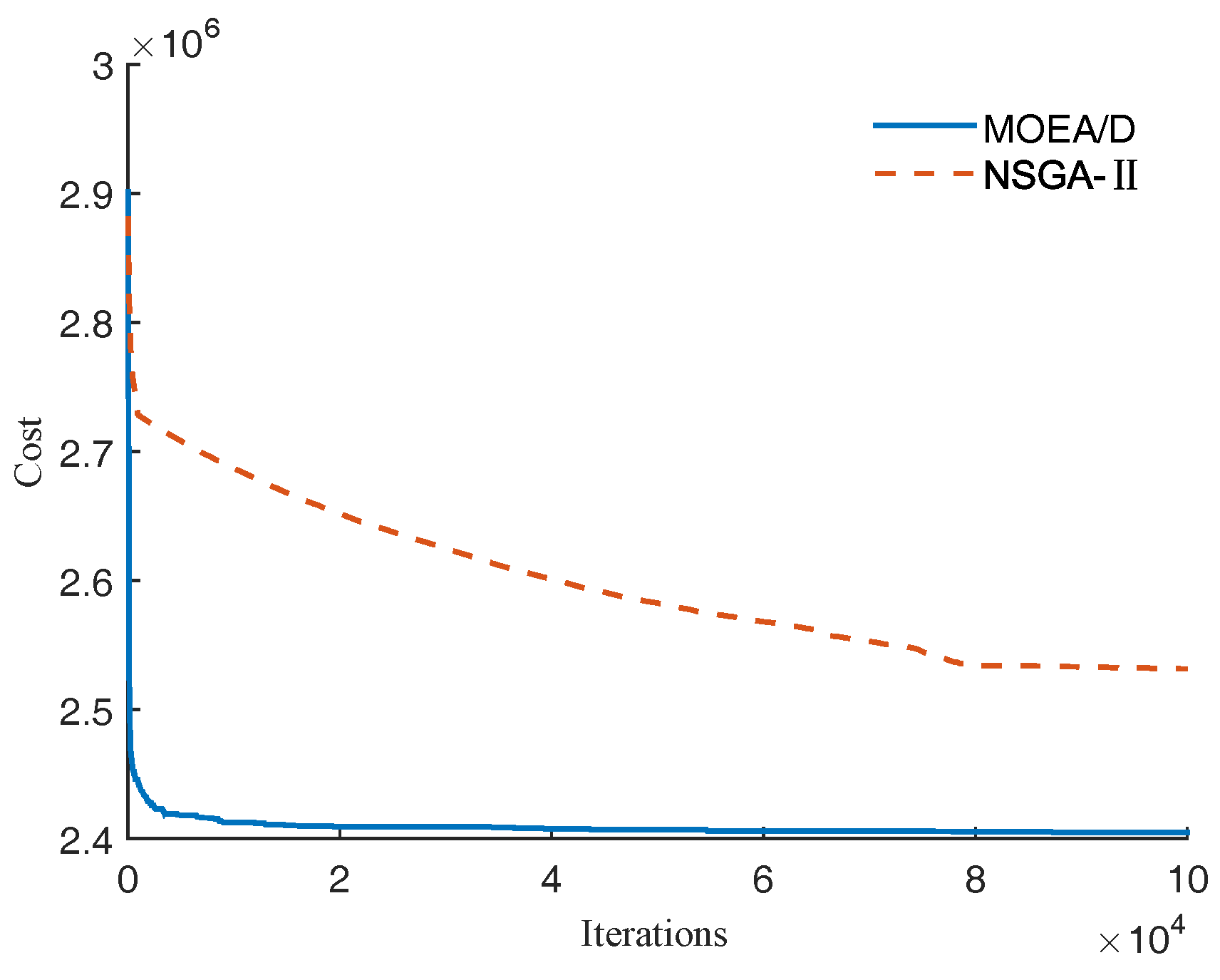
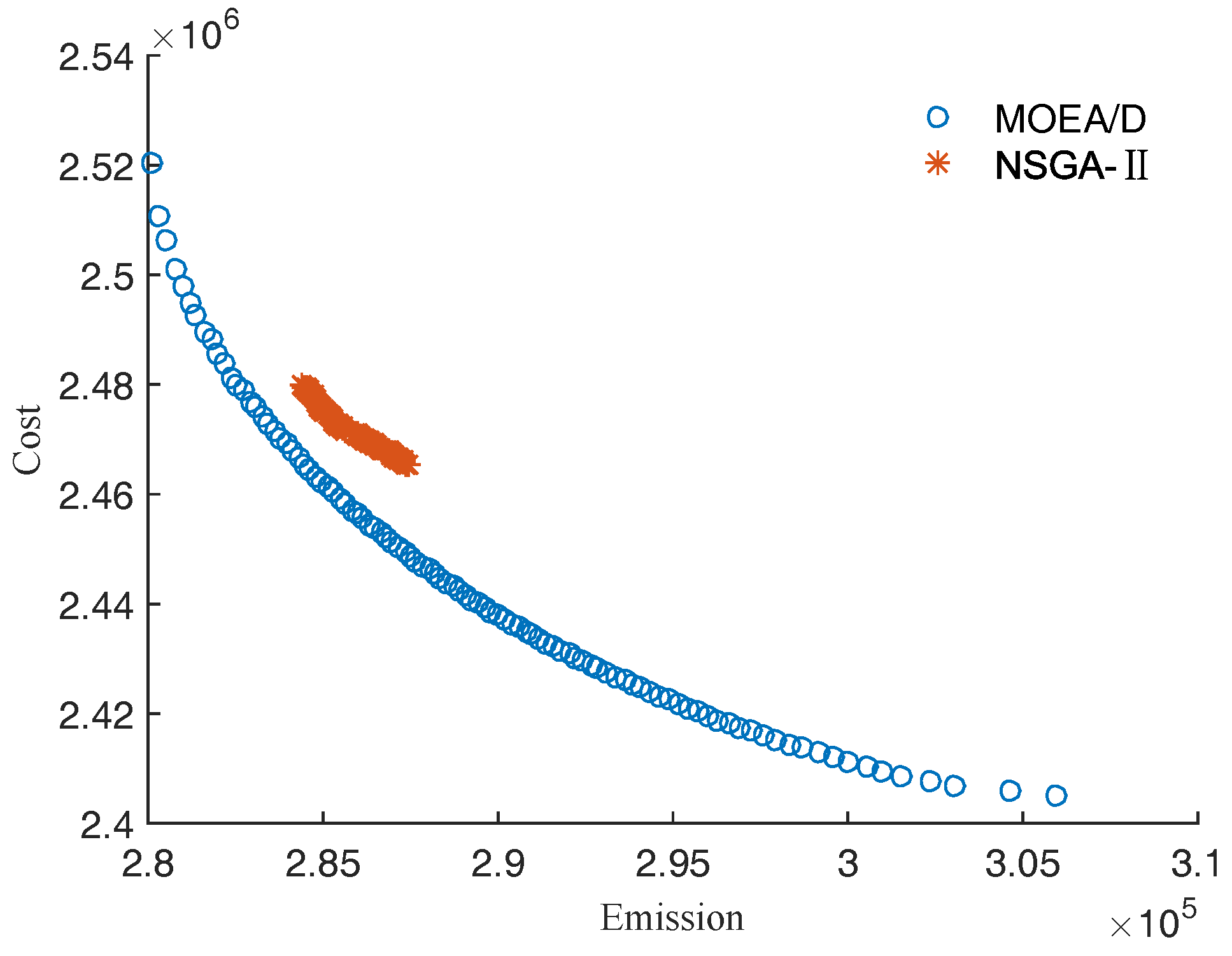
NSGA-II is a classical algorithm; however, it cannot obtain feasible solution with the same generations above. When increasing the generations to 10⁵, the NSGA-II could get a set of feasible solutions; MOEA/D also obtained a set of feasible solutions in the same condition. The results in

Table 4. The solutions and average computation time (seconds) of MOEA/D and NSGA-II (Iterations = 10⁵).

Methods	MOEA/D		NSGA-II
	Cost	Emission	Cost	Emission
Best cost	2.4050 × 106	3.0594 × 105	2.4653 × 106	2.8736 × 105
Best emission	2.5203 × 106	2.8007 × 105	2.4801 × 106	2.8436 × 105
Best compromise	2.4478 × 106	2.8765 × 105	2.4715 × 106	2.8560 × 105
Average time	39,345.24		44,827.5

show that the best cost and the best emission obtained by MOEA/D are lower by $0.0603 × 10⁶ and 0.0429 × 10⁵ lb compared with NSGA-II, respectively. For the best compromise solution, compared with MOEA/D, the emission obtained by NSGA-II was reduced by 0.0205 × 10⁵ lb; however, the cost increased by $0.0237 × 10⁶. In Figure 5, the PF distribution of the MOEA/D is even more uniform, which can help decision makers select the more reasonable dispatch schemes.

As can be seen from the results of the analysis, the extreme solutions obtained by MOEA/D are the best among all of the methods. When choosing the minimum cost dispatch scheme, MOEA/D can save a minimum of $0.0066 × 10⁶. When choosing the minimum emission dispatch scheme, MOEA/D can decrease emissions by at least 0.0429 × 10⁵ lb. It will provide a better choice for decision makers. The best compromise solution offers the trade-off relations between the best cost and the best emission in PF.

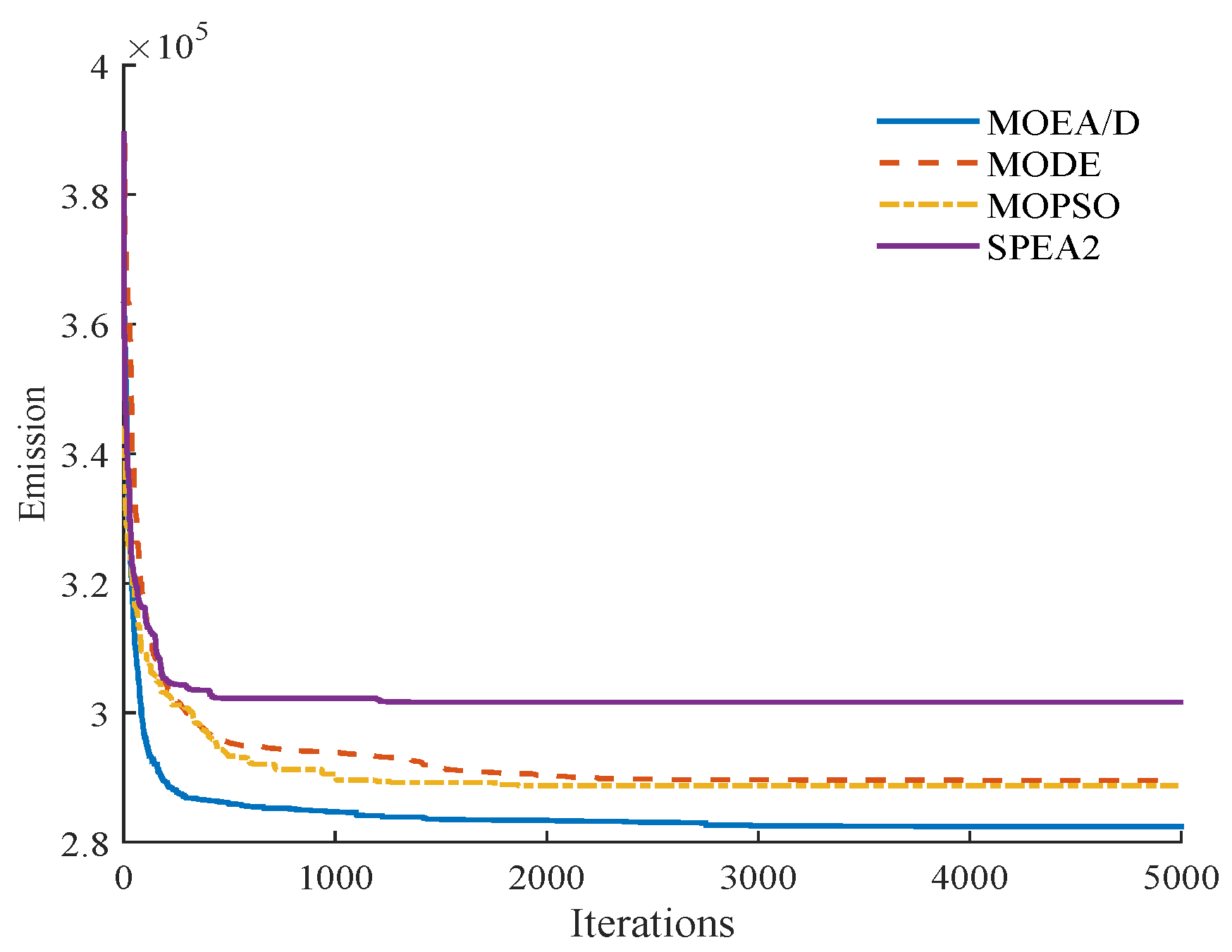
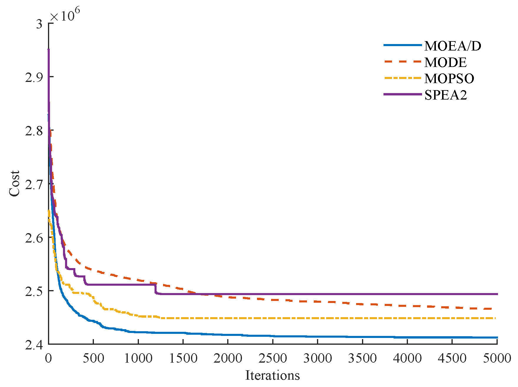
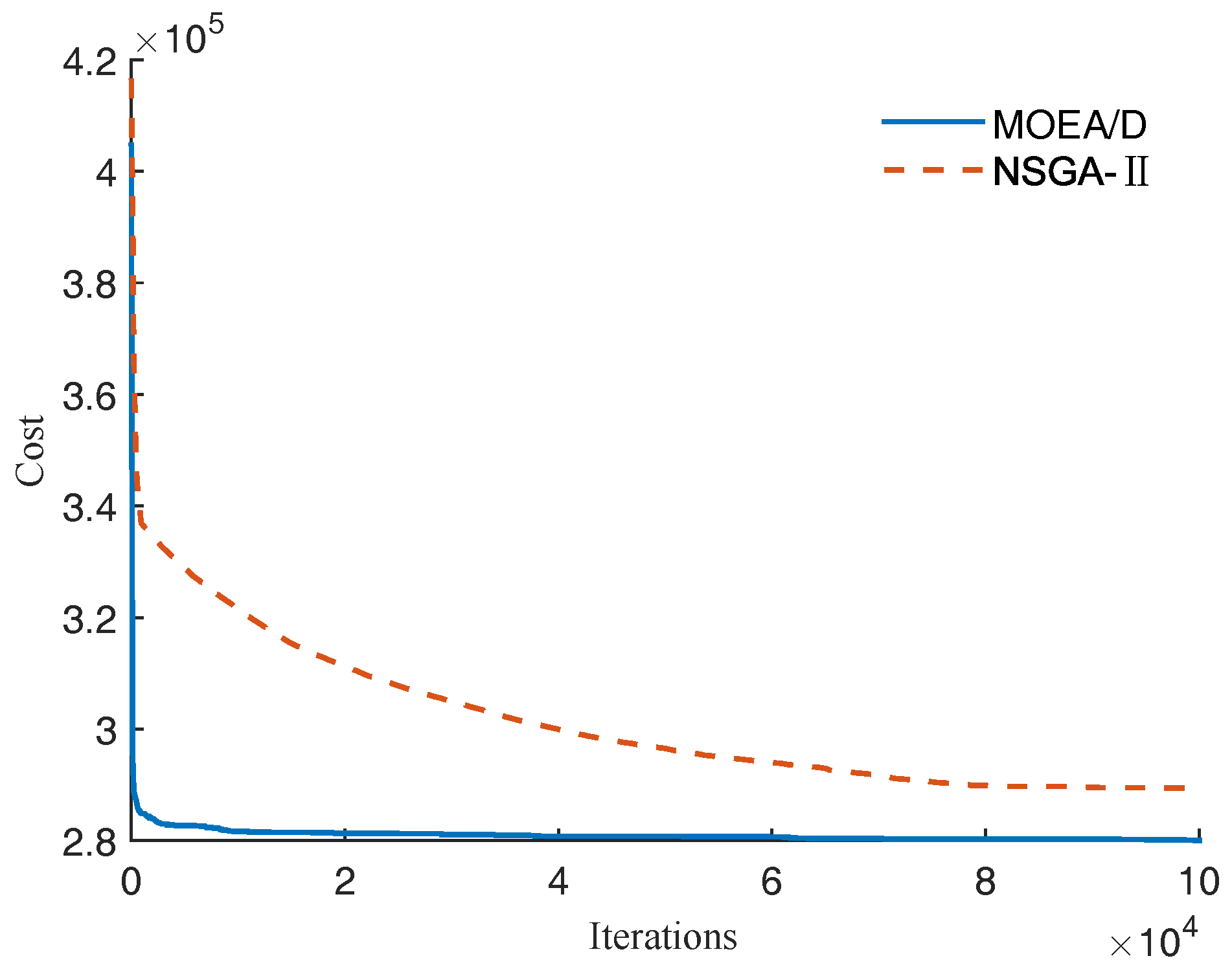
All five methods can obtain relatively integrated PF. However, compared with MODE, MOPSO, SPEA2 and NSGA-II, the proposed MOEA/D is much better. Due to its advantages in algorithm design, it performs well in search capability and solutions diversity. The solutions are well distributed and can provide the decision makers more and better choices. The convergence property of cost and emission in this dispatch system obtained by MOEA/D, MODE, MOPSO, SPEA2 and NSGA-II are shown in Figure 6, Figure 7, Figure 8 and Figure 9. In addition, Table 3 and Table 4 show that MOEA/D requires less computation time than the other methods with the same number iterations and population size for DEED problem.

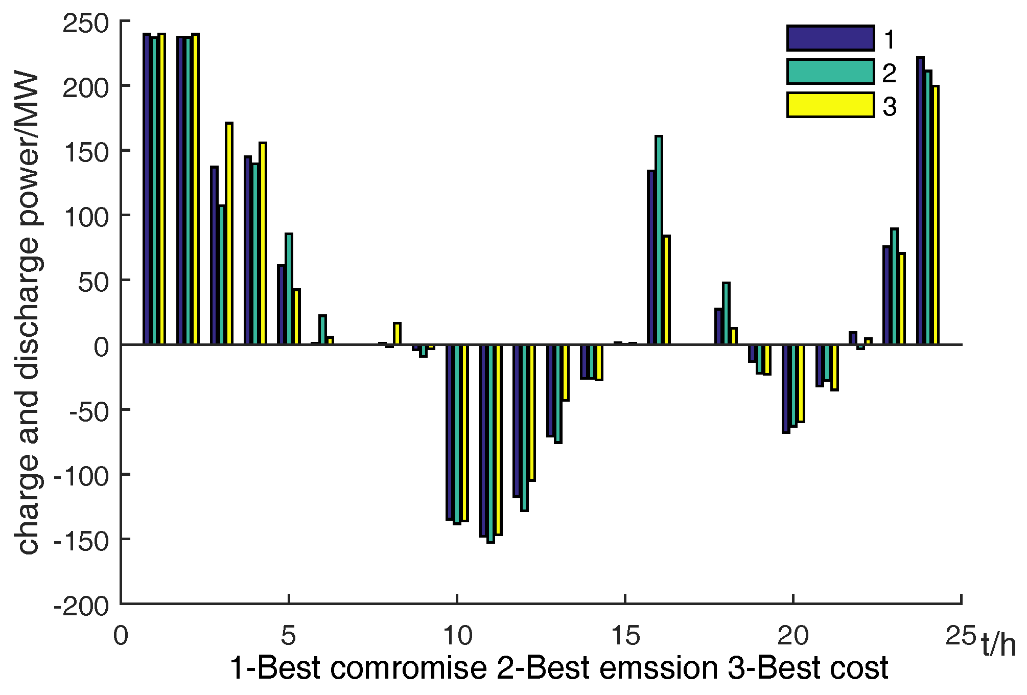
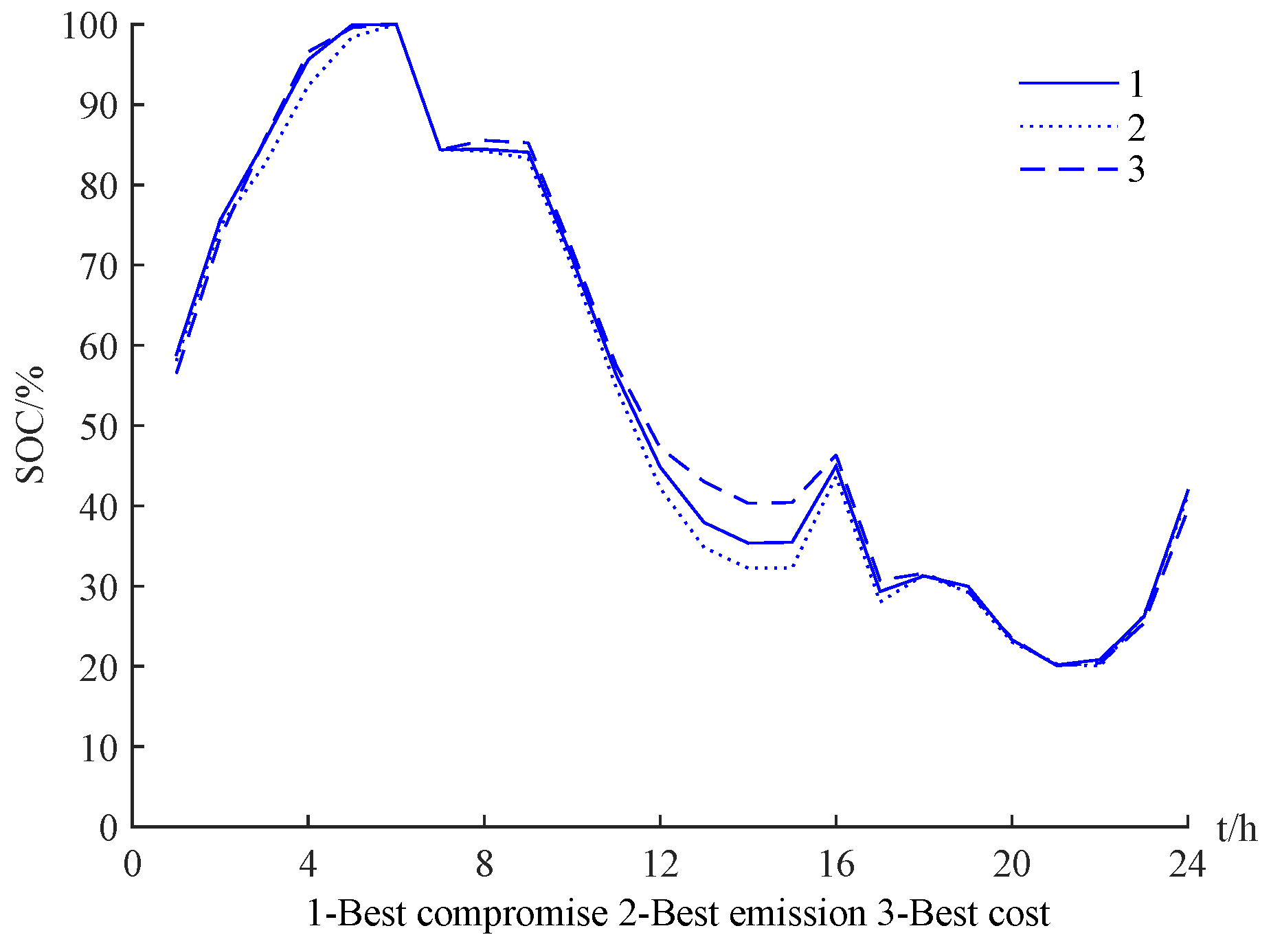
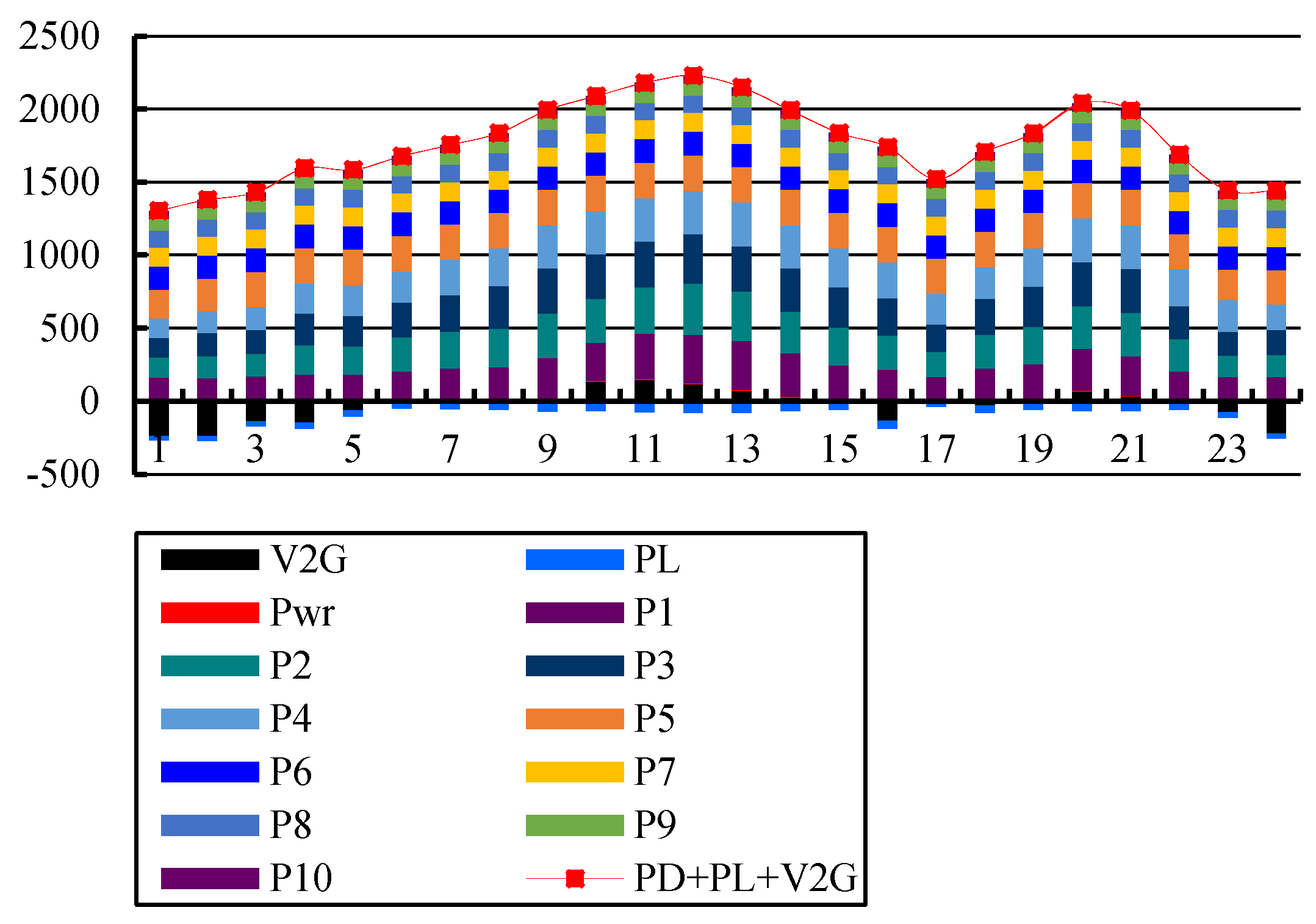
To verify the dispatch scheme, in Figure 10, comparison of EVs charge and discharge power among different solutions, and, in Figure 11, the EVs charge and discharge power and State of Change (SOC) under different schemes (in figure, time l represents 00:00–01:00, and so on) are illustrated. The output power of each generator and EVs charging and discharging power are shown in Figure 12.

Figure 10 and Figure 11 shows that the extreme solution and best compromise solution corresponding to the EVs charging and discharging rule is similar, only different on the specific power. It changes the load distribution among the conventional units, and, eventually, leads to a great difference in fuel costs and pollution emissions.

As it can be seen from the above results, the EVs during 22:00–06:00 are in charging status, and SOC reaches 100% by 07:00, which ensures the EVs travel demand. During 07:00–08:00, the EVs are driving on the road, with on-board battery discharging, leading to SOC falling. From 08:00 to 15:00 is the peak period of power consumption; the highest and the lowest loads are 2150 MW and 1776 MW, respectively. During this period, the EVs in the discharging state alleviate the pressure of the conventional thermal power units, and the SOC continues to fall. Since the driving needs of the owner occur during 17:00–18:00, the EVs are charging from 16:00, and the SOC rises. However, from 20:00 to 21:00 is the nighttime peak load, and the EVs continue to discharge to SOC reaching the lower limit. Then, EVs charge during the nighttime valley load until the next day trip.

5.2. Case 2

This case considers the impact of different EVs scale on DEED problem. Meanwhile, the parameters of MOEA/D and wind farm are the same as Case 1 and, referring to the wind power handling method in [41], the penetration level of EVs can be defined as:

$$p=\frac{P_{NCh}}{P_{D.peak}}\times 100\%$$

(35)

where P_D.peak is the peak load of the system. The extreme solutions and change trends of different penetrations are shown in

Table 5. Extreme solutions of different penetrations.

EVs	p/%	Objective	Cost	Emission
20,000	4.47	Best cost	2.4269 × 106	3.0172 × 105
		Best emission	2.5014 × 106	2.8646 × 105
30,000	6.70	Best cost	2.4254 × 106	3.0423 × 105
		Best emission	2.4963 × 106	2.8315 × 105
40,000	8.93	Best cost	2.4243 × 106	3.0419 × 105
		Best emission	2.5011 × 106	2.8387 × 105
50,000	11.16	Best cost	2.4238 × 106	2.9917 × 105
		Best emission	2.5090 × 106	2.8175 × 105
60,000	13.40	Best cost	2.4189 × 106	3.0006 × 105
		Best emission	2.5272 × 106	2.8148 × 105
70,000	15.63	Best cost	2.4220 × 106	3.0495 × 105
		Best emission	2.5164 × 106	2.8240 × 105
80,000	17.86	Best cost	2.4315 × 106	3.0312 × 105
		Best emission	2.5204 × 106	2.8317 × 105

and Figure 13 and Figure 14.

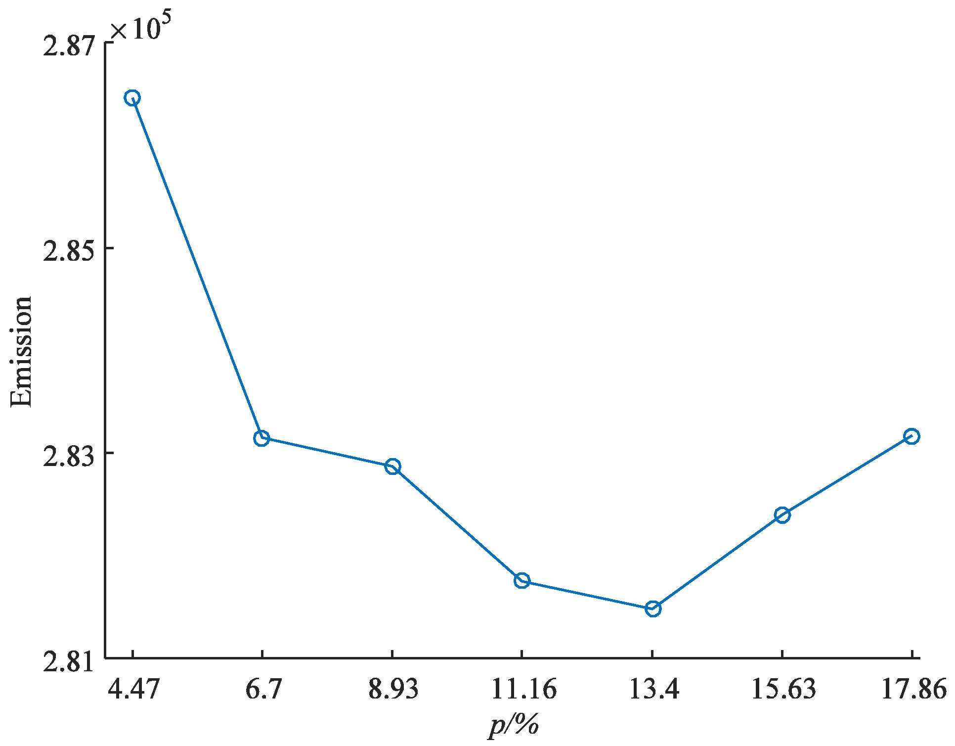
As the continuous expansion of the scale of EVs, the penetrations are increasing, and the corresponding optimal fuel cost and pollution emission will continue to decrease. Therefore, the EVs can be accessed to power grid by forming the V2G, which reduces the economic and environmental pressures of conventional thermal power units in initial stage. However, when the number of EVs reaches 60,000 (the penetration is 13.40%), the optimal fuel cost and pollution emission are reduced to minimum. On the contrary, as the scale of EVs keeps increasing, the optimal fuel cost and pollution emission also rise, which implies that the benefits to the economy and environment are weakening, with the penetration of EVs after reaching an inflection point. Instead, large scale EVs charging demand continues to increase, and the power system should sacrifice a certain amount of fuel cost and pollution emission for the extra charging load. Therefore, when considering the scale of EVs access to the power grid and setting the relevant dispatch planning, it is not simply that more EVs mean bigger benefit to the power grid. A comprehensive evaluation based on the actual situation of the power system should be conducted.

5.3. Case 3

Analyses of the wind farm parameters influence on the power system in DEED model will be given in this section. One hundred identical wind turbines are in the wind farm, and the v_in, v_out and v_rate are 3 m/s, 25 m/s and 15 m/s, respectively. The other parameters of wind turbines and thermal power generators are the same as Case 1. The total rated power of wind farm is 150 MW, and the scale of EVs is 50,000. The EVs and MOEA/D parameters remain unchanged. The load peak period of 2150 MW is selected to analyze the effect of three factors (confidence level η₁, shape factors k and scale factors c) on the power system.

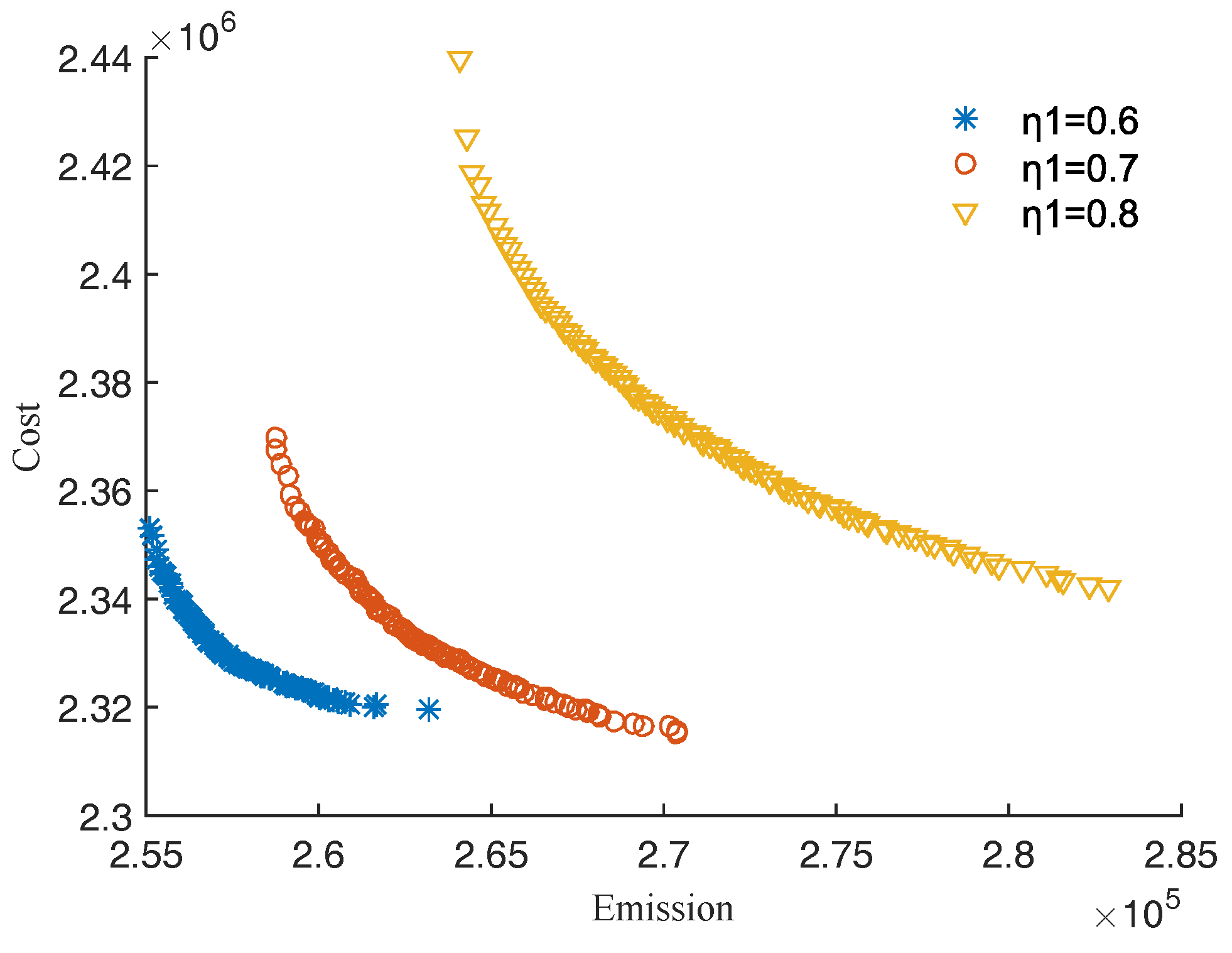
5.3.1. Different Confidence Level

Select the shape factor k = 2.2 and the scale factor c = 15 m/s to analyze the dispatch scheme of the confidence levels η₁ of 0.8, 0.7 and 0.6, respectively. The PF of the system obtained by different confidence levels is shown in Figure 15. The compromise solutions of generator output power at peak load and total cost and total emission in dispatch period obtained by different confidence levels are listed in

Table 6. Compromise dispatch schemes obtained by different confidence levels of ${\eta }_1$.

Parameters	${\mathit{\eta }}_{\mathbf{1}}$
	0.8	0.7	0.6
P1/MW	287.93	300.57	270.92
P2/MW	310.86	271.42	292.12
P3/MW	312.01	313.6	301.36
P4/MW	299.16	300	281.33
P5/MW	243	243	242.98
P6/MW	160	160	159.98
P7/MW	130	130	129.98
P8/MW	120	120	119.98
P9/MW	80	80	79.976
P10/MW	55	55	54.979
V2G/MW	−177.54	−175.8	−191.56
Pw/MW	45.6392	69.7958	91.1714
Total Cost/$	2.3777 × 106	2.3333 × 106	2.3295 × 106
Total Emission/lb	2.6915 × 105	2.6261 × 105	2.5727 × 105

.

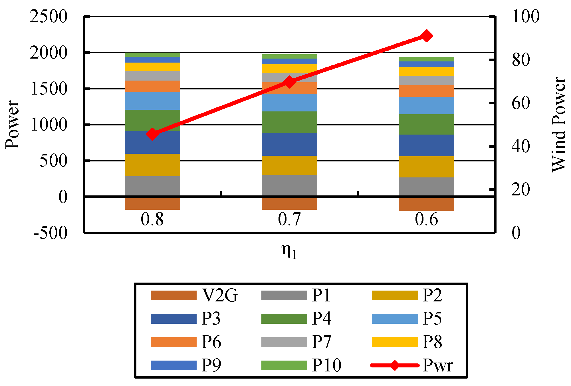
Table 6 and Figure 16 show that, with the decrease of the confidence level, the output of the wind farm increases monotonically. The total output power of generator unit in peak load is monotonically reduced. The total fuel cost is reduced by $0.0482 × 10⁶, while the total pollution emission is reduced by 0.1188 × 10⁵ lb. The result demonstrates that the increase in wind power effectively reduces fuel cost and pollution emissions. However, it also brings greater security risks for the safe operation of the power system. Therefore, decision makers should choose the right scheme according to need.

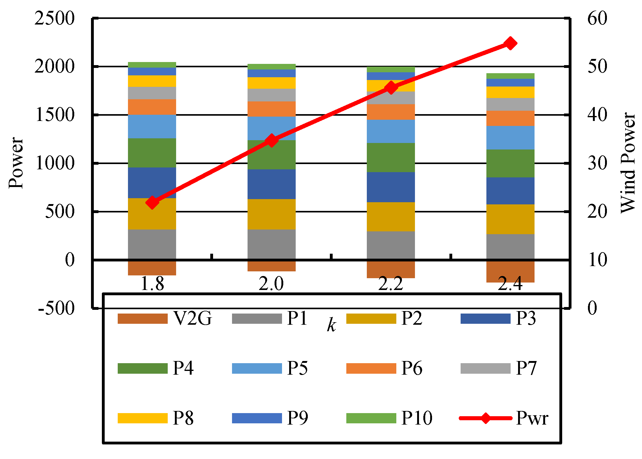
5.3.2. Different Shape Scale

Select the confidence level η₁ = 0.7 and the scale factor c = 15 m/s. The shape parameter of k is selected as 1.8, 2.0, 2.2 and 2.4, respectively, for optimizing the DEED model. The PF of the power system shown in Figure 17 is obtained by different shape scale. The compromise solutions at the peak load and total fuel cost and pollution emission obtained by different shape scale are listed in

Table 7. Compromise dispatching schemes obtained for different shape factors.

Parameters	k
	1.8	2.0	2.2	2.4
P1/MW	318.01	315.8	296.75	267.22
P2/MW	323.3	315.1	302.73	307.97
P3/MW	317.79	308.15	301.61	281.01
P4/MW	299.91	299.99	299.97	287.29
P5/MW	242.89	242.9	242.87	242.85
P6/MW	159.9	159.66	159.97	159.7
P7/MW	129.58	130	129.91	129.85
P8/MW	119.85	119.93	119.86	119.86
P9/MW	79.84	79.999	79.964	80
P10/MW	54.897	54.998	54.866	54.785
V2G/MW	−157.25	−116.19	−186.37	−230.9
Pw/MW	21.8754	34.7046	45.6392	54.8138
Total Cost/$	2.4296 × 106	2.3999 × 106	2.3814 × 106	2.3665 × 106
Total Emission/lb	2.7904 × 105	2.7483 × 105	2.6848 × 105	2.6563 × 105

.

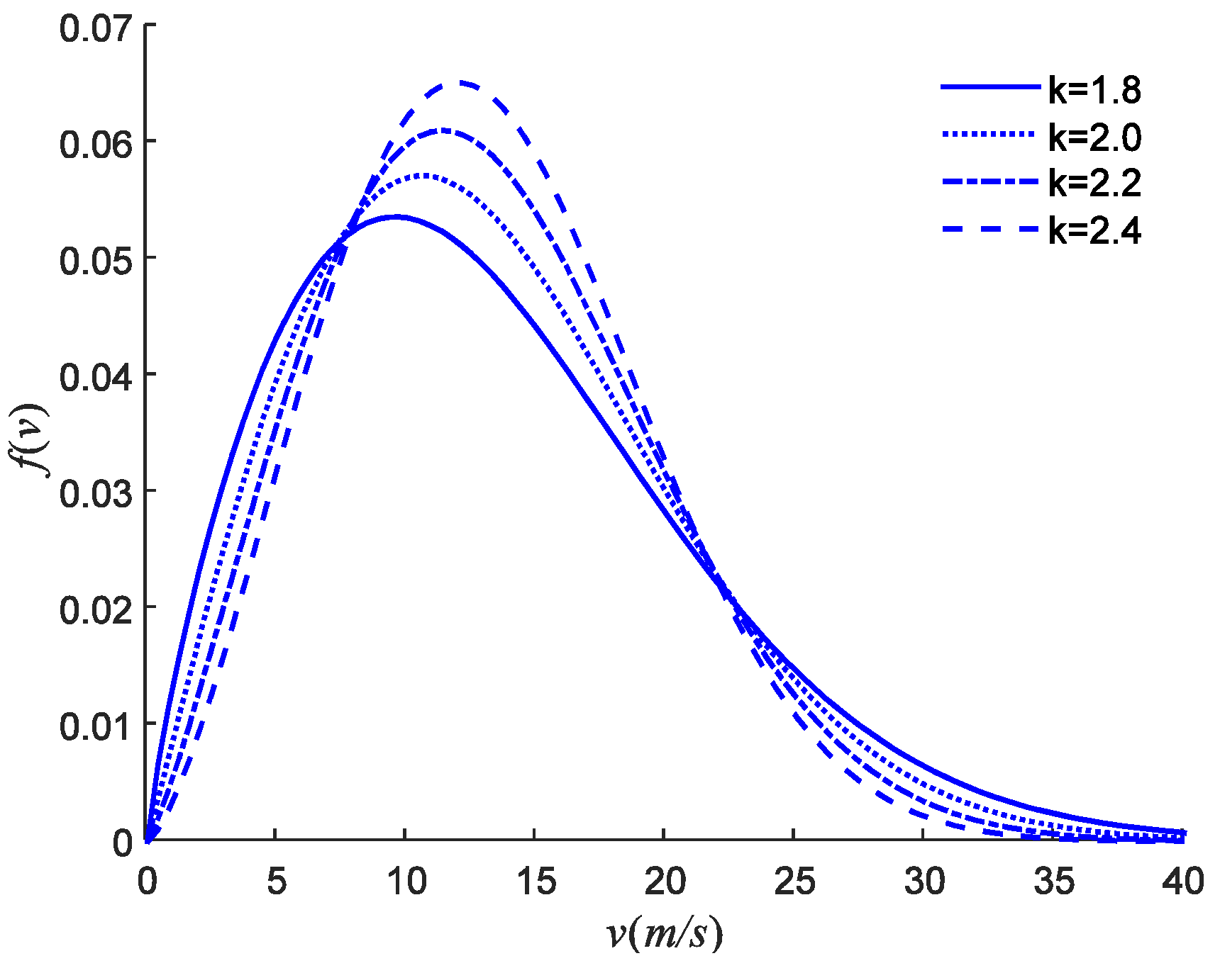
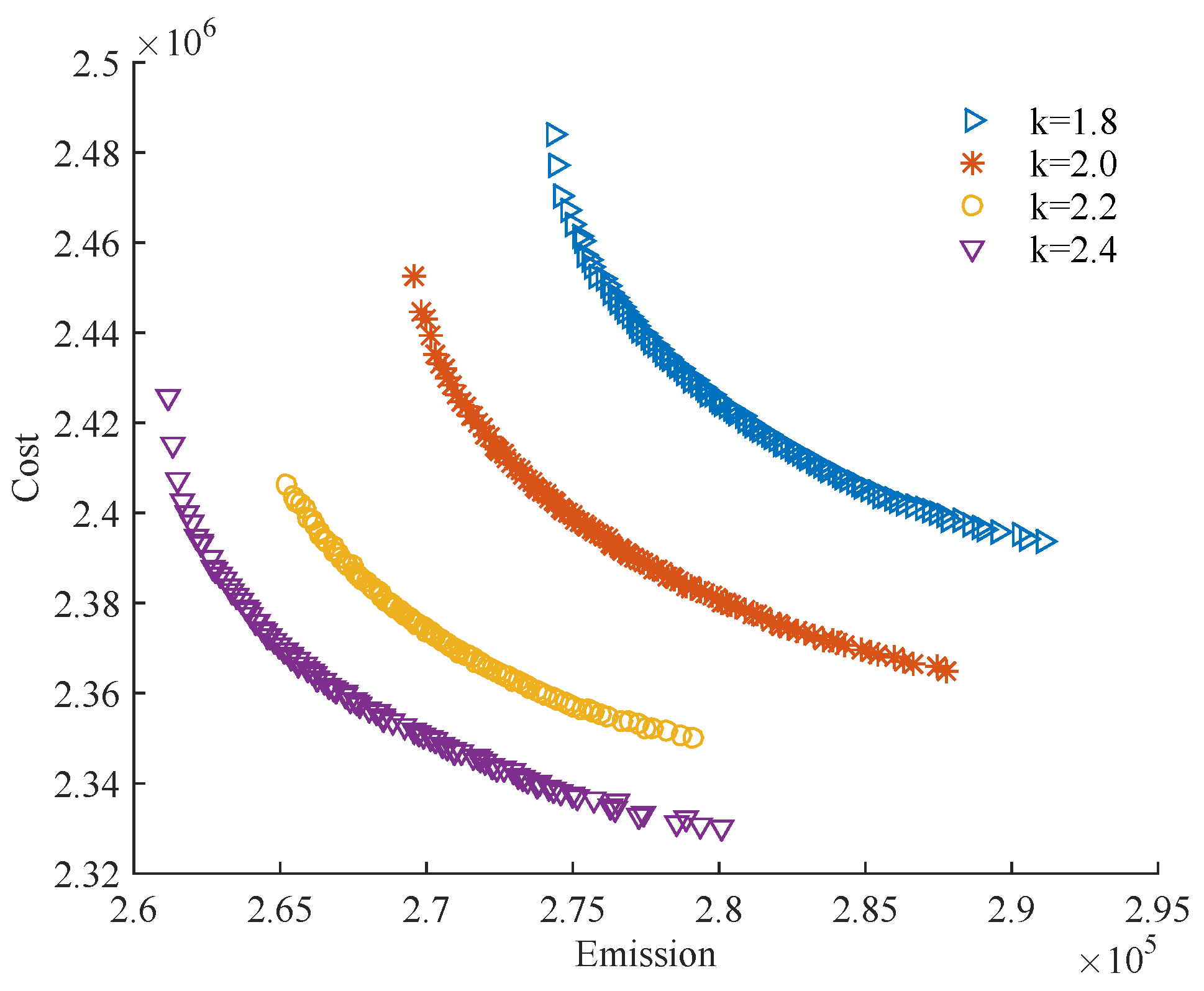
Table 7 and Figure 18 show that the output power of the wind farm increases monotonically as the shape scale increases. Meanwhile, the total output power of generator unit in peak load is monotonically reduced. The total fuel cost reduces from $2.4296 × 10⁶ to $2.3665 × 10⁶, and the total pollution emission reduces from 2.7904 × 10⁵ lb to 2.6563 × 10⁵ lb at the same time. Due to the variation of the wind speed PDF in different shape factors, Figure 19 shows that, in the vertical direction, with the increasing of k, the PDF curve of wind speed becomes steeper gradually and the peak value increases. With the increasing of wind speed, the corresponding peak value increases gradually. It suggests that the wind speed distribution is more concentrated near the probability peak of wind speed with increase of shape factors. Therefore, within the rated power range, the output of the wind farm increases correspondingly.

5.3.3. Different Scale Factors

Select the confidence level η₁ = 0.7 and the shape factor k = 2.0 to calculate the dispatch scheme where the c is 13 m/s, 16 m/s, 19 m/s and 21 m/s, respectively. The PFs of the system obtained by different scale are shown in Figure 20, and the compromise solutions at the peak load and total fuel cost and pollution emission obtained by different scale are listed in

Table 8. Compromise dispatching schemes obtained for different scale factors.

Parameters	c/(m/s)
	13	16	19	21
P1/MW	255.73	311.05	317.81	334.27
P2/MW	313.81	307.54	356.38	324.16
P3/MW	284.79	304.7	339.52	334.24
P4/MW	299.33	299.71	300	299.99
P5/MW	243	243	242.99	242.95
P6/MW	160	159.96	159.97	159.96
P7/MW	130	129.96	130	129.98
P8/MW	119.9	120	120	119.98
P9/MW	80	79.898	79.928	79.989
P10/MW	55	55	54.986	54.989
V2G/MW	−220.67	−151.12	−79.442	−120.89
Pw/MW	54.6970	60.3730	48.5219	26.4460
Total Cost/$	2.4097 × 106	2.3573 × 106	2.3250 × 106	2.4215 × 106
Total Emission/lb	2.7644 × 105	2.6339 × 105	2.7232 × 105	2.7924 × 105

.

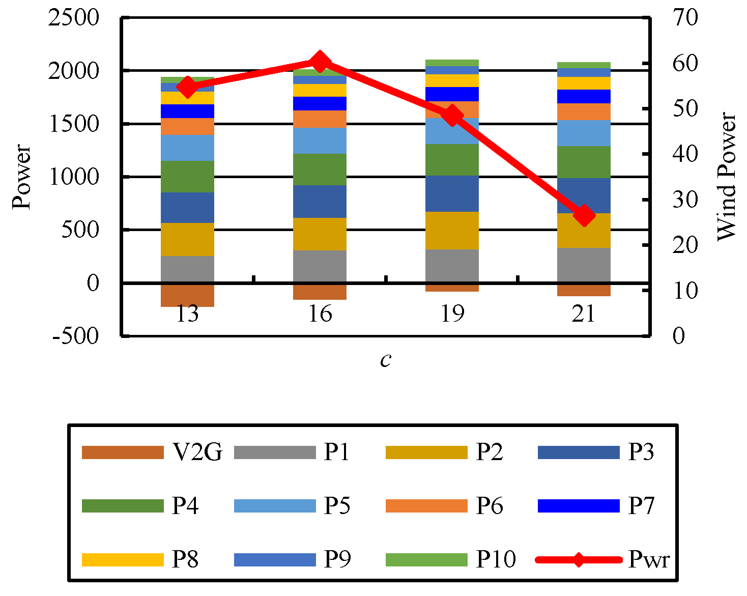
The scale factor represents the average wind speed, which determines the active power of the wind farm. However, as shown in Table 8 and Figure 21, the output of the wind farm does not increase monotonically, but displays an increasing trend at first and then a decreasing trend as c increases. The total fuel cost and emission all decrease at first and then increase.

The above results indicate that, as the load demand of confidence levels decline and the shape factors increase, the output of wind farm increases monotonically. With the increase of scale factors, the output of wind farm increases at first, and then decreases. Hence, this trend is in line with the real characteristics of wind turbines that, with the increasing of the wind speed, the wind turbine’s output power increases at first and then decrease [42].

5.4. Case 4

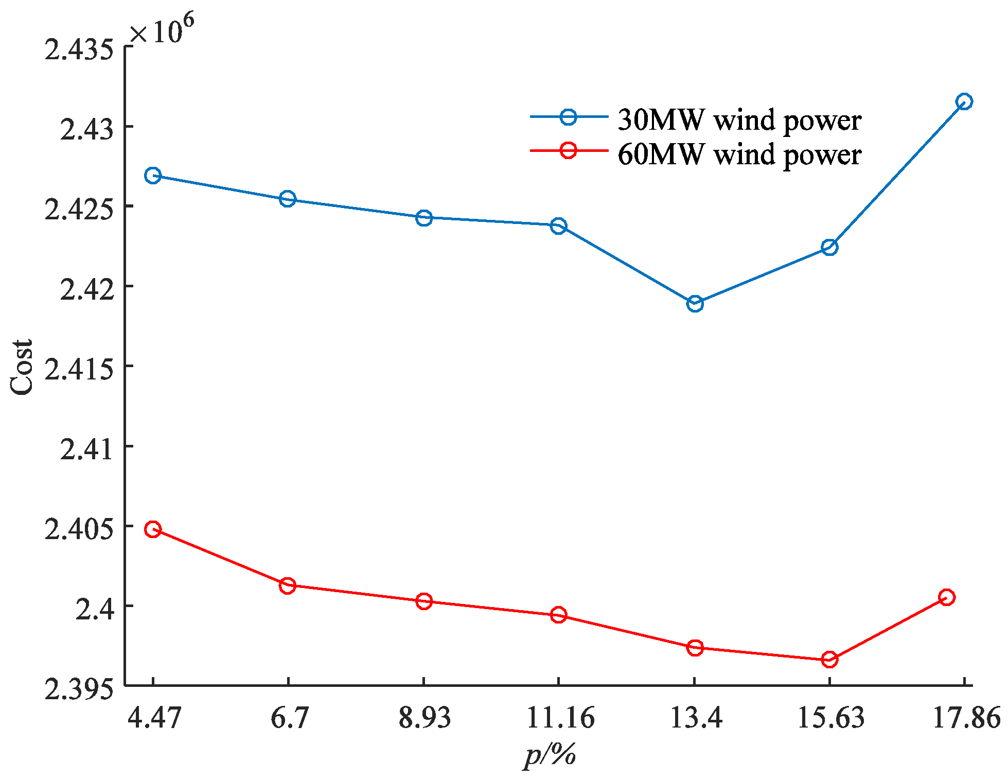
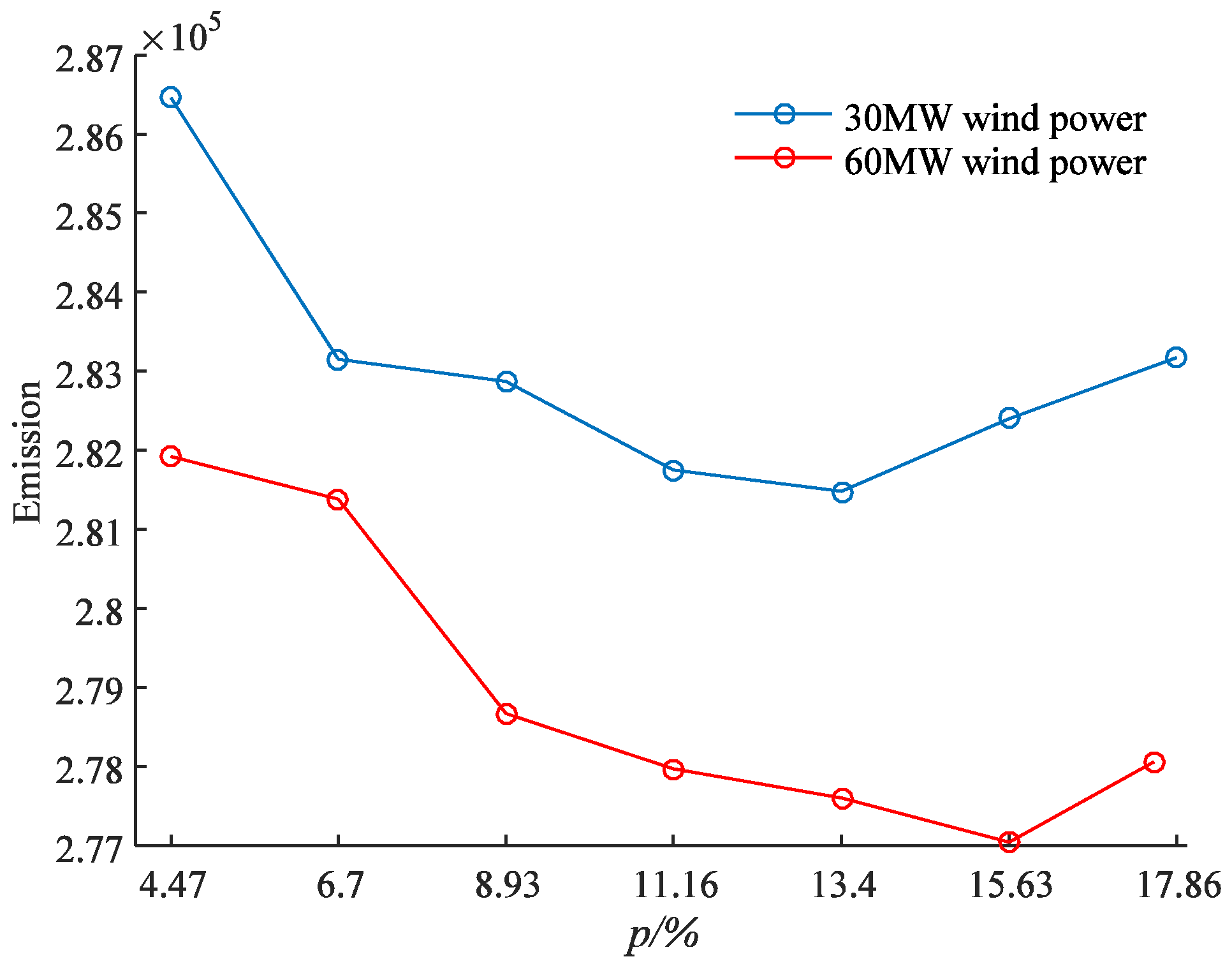
From the result of Case 2, we can see that, with the increase of the number of EVs and the resulting increase of the load of the power grid, the stability of the power grid is adversely affected. Based on Case 2, wind turbines in the wind farm have been doubled, i.e., the rated output of the wind power is changed to 60 MW. Other parameters of wind farm and thermal power generators remain unchanged. Similar to in Case 2, the scale of EVs accessing the power grid dispatch is from 20,000 to 80,000. The EVs and MOEA/D parameters are consistent with the cases above.

The results of the optimization are listed in

Table 9. Extreme solutions with different penetrations at two times wind power.

EVs	p/%	Objective	Cost	Emission
20,000	4.47	Best cost	2.4048 × 106	3.0089 × 105
		Best emission	2.4821 × 106	2.8192 × 105
30,000	6.70	Best cost	2.4013 × 106	2.9606 × 105
		Best emission	2.4846 × 106	2.8138 × 105
40,000	8.93	Best cost	2.4003 × 106	2.9703 × 105
		Best emission	2.4962 × 106	2.7867 × 105
50,000	11.16	Best cost	2.3994 × 106	2.9679 × 105
		Best emission	2.4870 × 106	2.7797 × 105
60,000	13.40	Best cost	2.3974 × 106	2.9624 × 105
		Best emission	2.5133 × 106	2.7760 × 105
70,000	15.63	Best cost	2.3966 × 106	3.0400 × 105
		Best emission	2.5035 × 106	2.7704 × 105
80,000	17.86	Best cost	2.4005 × 106	3.0542 × 105
		Best emission	2.5166 × 106	2.7806 × 105

. When the number of EVs is 20,000, the extreme solutions of best cost and best emission were reduced by $0.0221 × 10⁶ and 0.0272 × 10⁵ lb, respectively, compared with Case 2. When the penetration is 13.4%, i.e., the number of EVs is 60,000, which is the inflection point of the permeability in Case 2, the best cost decreased by $0.0224 × 10⁶ and the best emission was reduced by 0.03888 × 10⁵ lb compared with Case 2. When the scale of EVs is 70,000, the fuel cost and the pollution emission increase compared with 60,000 in Case 2. In this section, however, the fuel cost and the pollution emission continue to decline. They were decreased by $0.0008 × 10⁶ and 0.0056 × 10⁵ lb, respectively, compared to 60,000. Moreover, when the scale of EVs increases to 80,000, the corresponding extreme solutions also increase by $0.0039 × 10⁶ and 0.0102 × 10⁵ lb compared with 70,000, which indicates that the inflection point value of the EVs penetration becomes 15.63% at two times the wind power. The corresponding extreme solutions with the penetrations curve are shown in Figure 22 and Figure 23.

From the above analysis, it can been see that the increased in wind power, to a certain extent, relieves the pressure to the power system load caused by the large scale EVs: the inflection point of EVs rises from 13.40% to 15.63%. Therefore, the proper rise of wind power would increase the number of EVs, while reducing the economic and environmental pressure of the power system. Furthermore, comparing Case 3 with Case 2 shows that interaction exists between EVs and wind power. Therefore, the decision makers can appropriately increase the number of EVs and the output of the wind farms as needed. It also provides a way for decision makers to be involved in co-scheduling with electric vehicles and wind power.

6. Conclusions

In this paper, a novel multi-objective DEED model is formulated to consider EVs and wind power. When dealing with the wind power uncertainty, this paper uses the Weibull probability distribution function. For EVs charging and discharging control, we carry out the double-layer dispatch strategy. To solve the high dimension DEED problem with various constraints, this paper has improved the standard MOEA/D by employing a two-step constraint processing method based on dynamic adjustment of decision variables. A 10-unit system with 50,000 registered EVs and one wind power farm is tested and a series of Pareto optimal solutions are obtained. Moreover, the performance and the effectiveness of the proposed method are examined on four power systems. From the comparison of numerical results, it is known that the improved MOEA/D has a better convergence performance and can obtain more uniformly distributed PFs than the other algorithms. From the results of the case study, this work obtained the impacts of EVs charging/discharging and wind power on power grids, as well as their mutual influence. Finally, we obtained the impact of wind power parameters on the PDF, which provided a novel thought for wind power grid connection. The formulation present in EVs is focused on charging/discharging process and users demand. However, battery cost and battery degradation are key factors in the overall price of EVs. Our future work will consider different charging/discharging policies, battery cost and management services cost that are more consistent with the real situation. Another important avenue for future research is to analyze the constraints handing method and improve other multi-objective optimization algorithms.