1. Introduction
The production of energy from wind has become economically and technically viable, with high potential for growth. However, the uncertainty associated with production forecasts, linked to the stochastic nature of wind, is a critical issue for the existing distribution networks, due also to the increased supply of power generation from other renewable sources [
1].
The problem becomes even more evident if the grid is small and possibly not connected to the distribution and transmission network. This is particularly the case on small islands, where the introduction of renewable sources requires particular attention because of the limited size of the distribution grid and of the concentration of the production [
2].
To reduce the negative impact of the variability of energy production from renewables, in particular from wind power, different strategies can be applied: geographical dispersion of the production plants, load management, temporary power production cuts, energy storage and wind power forecast (WPF). Energy storage and generation forecasts are the most attractive strategies for a small grid, and in particular for use on an island. These procedures are one of the subjects studied in the European NETfficient project (
http://www.netfficient-project.eu), to which this work is related. The project aims to propose effective innovation on the use and distribution of electric power through the development of several energy storage technologies and an energy management system, enabling the implementation of a smart grid on the German island of Borkum in the North Sea.
The improvement of the forecasting techniques for the power produced by wind turbines is essential for an increase in network input and an optimal sizing of the storage capacity required for grid stability. To this end, an accurate forecast is critical as well as knowing the uncertainty associated with that prediction [
3].
It’s hard to compare the many different techniques that have been developed over the years to predict turbine power from wind velocity, due to the peculiarities of each application, which depend on the type of installation, geographic characteristics, time horizons of interest, and also on the purpose for which a prediction is required. A recent and complete review of the techniques proposed in the literature can be found in [
4].
The estimated power production is the output of the representative model of the turbine, which, according to the forecasting technique used, can receive, as input, different types of weather variables, which in turn are the output of some Numerical Weather Prediction (NWP) models.
The simplest way of building a turbine model is to obtain a functional relationship between produced power and wind speed. This model can be supplied directly from the manufacturer or derived by applying regression techniques to historical data series of electric power and wind speed simultaneous observations, and in this case is known as the wind turbine power curve.
The power curves provided by turbine manufacturers are valid for a brand new turbine in standard ideal conditions. Wind turbines seldom operate under such conditions [
5], and there is often a discrepancy between the empirical and theoretical power curve, which results in inaccurate power prediction and motivates some research works in the recent years [
3,
6,
7].
The forecasting models presented in the literature are usually divided in parametric and non-parametric.
The parametric models are built from a set of mathematical equations that include some parameters that have to be determined through regression methods from the available data for weather conditions and power generation [
3]. Through the years many parametric models have been proposed, examples include: the piecewise linear model [
8,
9], polynomial power curve of various degrees as discussed in [
10,
11], the maximum principle method by Rauh as proposed in [
12], the dynamical approach using the Langevin Model presented in [
12], a probabilistic method proposed in [
13], the so-called ideal power curve [
14], four and five parameters logistic functions [
5,
15] , as well as Modified hyperbolic tangent (MHTan) function [
6].
With the recent availability of powerful database tools for the management of large amounts of data, the non-parametric methods emerged. These methods instead of assuming a physical or analytic relationship between the input and output data, establish a correlation based only on the data provided.
Among these, the following can be recalled: the copula power curve model [
16], cubic spline interpolation [
9], different types of artificial neural network [
8,
10,
17,
18,
19], multi-layer perceptron, random forest, k-nearest neighbors and support vector machines [
8,
15,
20]. Among the non-parametric methods, there is the Method Of Bins on which the IEC 61400-12-1 standard is based [
21]. This standard is the most prescribed method for power performance evaluation of wind turbines.
All these methods are based on a set of simultaneous data on wind conditions and measured power. When the turbine model is constructed from Supervisory Control And Data Acquisition (SCADA) system measurements, the resulting model can be used for forecasting purposes only through a statistical postprocessing of the wind speed forecast obtained from the NWP systems, to have a reasonable estimation of the wind at the hub of the turbine. If the model serves only for forecast purposes, the power measurements may be directly related to NWP’s output, without the need of using the wind speed at the hub as an intermediate variable.
In this paper a simple but effective modeling technique for wind power forecasting is introduced, having several distinctive features:
It is based on the correlation between measured power and NWP wind speed forecast, specifically their probability distributions, and thus includes implicitly some of the influences of the local terrain and environment;
A good model can be obtained from a set of a few hundred of independently taken power measures and wind speed forecasts;
In spite of its simplicity, the results obtained are comparable and, when mean absolute error is used as an error measure, better than those obtained using other much more complicated and computationally expensive methods;
The approach could, in principle, also be applied to wind speed and generated power data observed in separate campaigns, with different sample rates, as long as the measured sets have significant statistical representativeness;
The remainder of this paper is organized as follows. The problem and the available datasets are described in
Section 2. The method is presented and discussed in
Section 3.
Section 4 introduces the accuracy metrics that are applied in the evaluation of the results, presented and briefly discussed in
Section 5. Finally, the conclusions are drawn in
Section 6 and some directions for future research are also given.
2. Observational and Forecast Data Sets
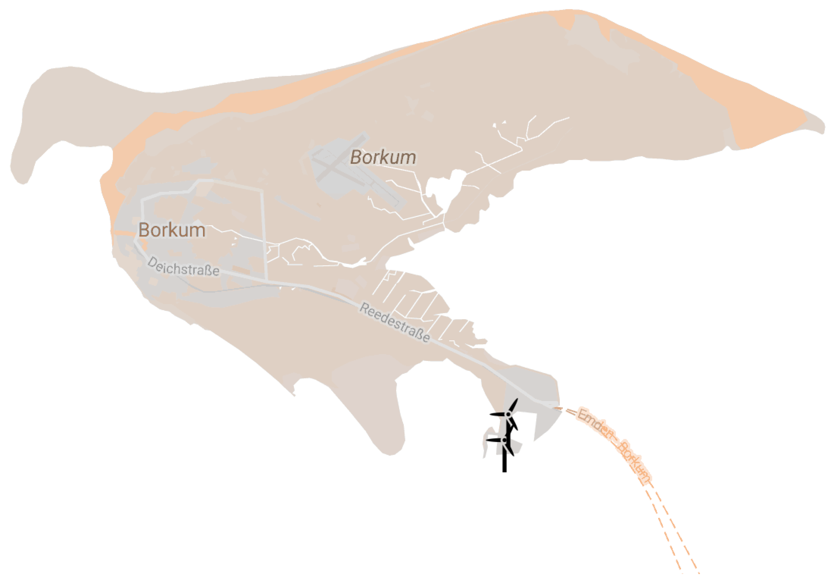
The problem consists in forecasting the electrical generation of two turbines located on the island of Borkum in Germany (
Figure 1). The two pitch controlled turbines (from the manufacturer Enercon) are identical, have a nominal power of 1.8 MW, a rotor diameter of 66 m, and are approximately 400 m apart. The manufacturer suggests installation heights for the hub between 68 and 114 m. The declared cut-in speed is 2.5 m/s, the cut-out speed is 34 m/s, and the rated speed is 12.5 m/s.
The observed data consists of one year (2014) of power measurements, with a frequency of 15 min. In-situ wind speed measurements are not available.
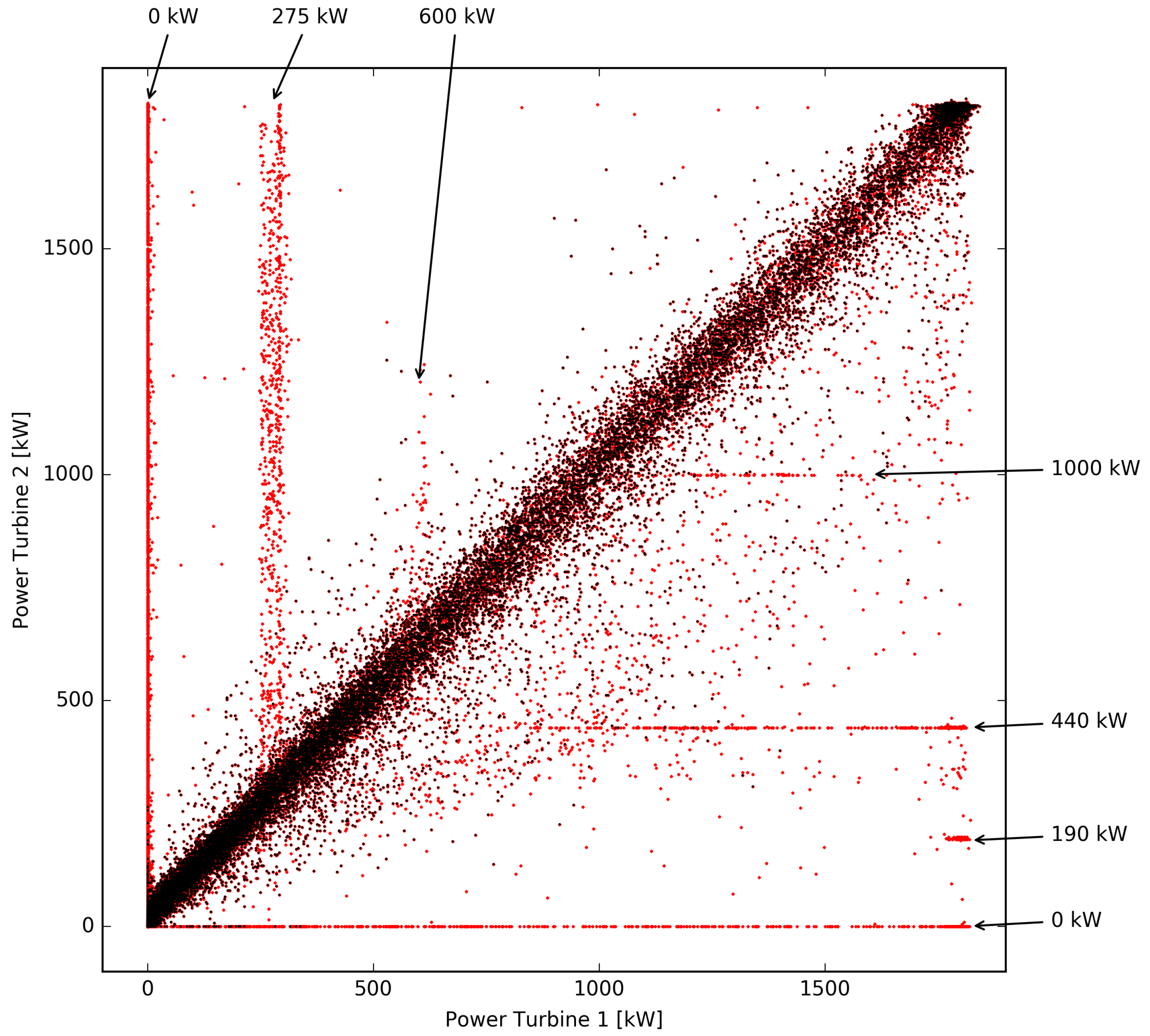
Given the relative proximity and the almost flat shape of the island, one can expect that the two turbines, sharing the same meteorological condition, must have very similar performances. In the
Figure 2, the scatter-plot of power measures for the two turbines is shown for each measurement available, using red dots.
As expected, the two data sets are very similar, but a more careful analysis reveals that, at least for wind speeds in a medium to high range, the power developed by turbine 1 systematically overrides the other. This fact can be related to a different level of efficiency of the two turbines, to a deterioration in performance due to use, or small differences in the local wind field.
The
Figure 2 highlights with arrows the instances where the power produced by the two turbines is significantly different, for reasons that can be related to temporary turbine malfunctioning or because the maximum output power is limited (power curtailment). Specifically, the plateaus of produced power (indicated by the arrows at the edge of
Figure 2) at about 0, 275 and 600 kW for turbine 1 and 0, 190, 440 and 1000 kW for turbine 2, can be noticed. This data has to be filtered out from the performance evaluation of a prediction system [
6]. The filtering operation was performed using the information provided by the turbines operator, and filtered data sets are represented in
Figure 2 with black dots. It is clear that, without a proper filtration procedure, any energy production forecasting method would have been biased because, in power-curtailment conditions, there is no direct link between the wind conditions and the power produced.
The power measurements were sub-sampled at a frequency of one hour, corresponding to the resolution of the weather forecast.
The weather forecasts of the wind speed at 100 m from the ground (height level that is most representative of the effect of the wind on the turbine) at 10 m and of wind gust are provided by the operative model (OP) of the ECMWF [
22]. In 2014, the ECMWF OP model was the TL1279L137 (horizontal resolution equivalent to approximately 14 km at medium latitudes with 137 vertical levels). The data were collected from the ECMWF MARS archive for 00GMT analysis and forecast time up to 48 h with a prediction interval of 1 h.
The wind speed was interpolated from the values on the nearest four grid points with weights inversely proportional to the distance.
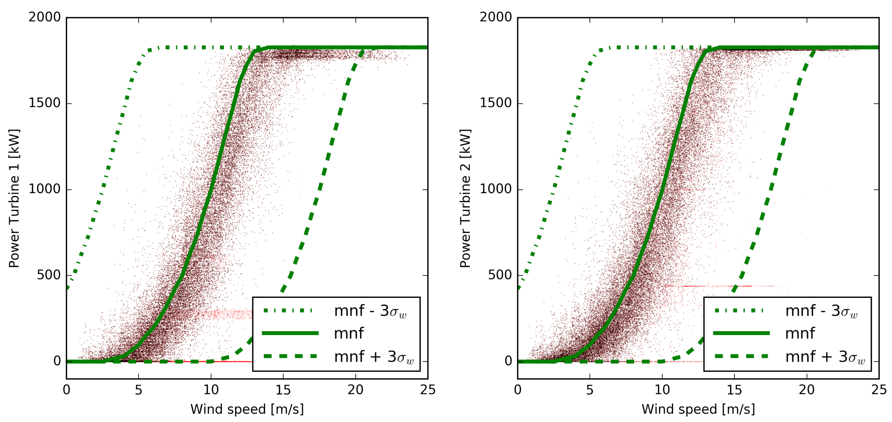
The
Figure 3 shows the measured power as a function of the wind speed forecast of the ECMWF model with the manufacturer’s power curve (mnf) in green, overlapped. It is evident that values corresponding to a power curtailment or where the turbines have been switched off have been appropriately filtered, as already evident from
Figure 2. In both figures, the presumable configuration of the power curve that relates wind speed and power produced is apparent. It is also apparent that there are wind speed and power pairs that significantly deviate from any plausible regression curve. These deviations can be due to power measurement errors, to modifications of the standard operation of the turbines not reported by the operator, and, of course, to wind speed forecast errors of the meteorological model.
It is perhaps useful to point out that a standard filtering procedure based on the direct relationship between produced power and wind speed, such as that described for example in [
6], is virtually ineffective in our case, once the wind speed forecast error are considered. Taking, in fact,
= 2.5 m/s as representative of the 48-h wind forecast uncertainty of the ECMWF model [
23] and using a
range around the manufacturer’s curve (which to a first approximation can be considered representative of the turbine’s behavior) we would obtain a range of uncertainty such as that represented by the area between the green curves in the
Figure 3. It can be seen that, at least in this case, the uncertainty of the wind estimate is such as to make practically any value of the measured power plausible.
3. Distribution Mapping Power Forecast
3.1. Introduction
Many techniques have been proposed in the literature for the construction of an efficient turbine model, integrating weather data measured in-situ or predicted from NWP models, with measures of the recent power generation.
The most straightforward model is known as the power curve. It relates generated power to wind speed at the height of the hub and can be formalized both as a lookup-table between discrete wind speed and corresponding power values or through a continuous analytic function.
The turbine builder often provides an estimate of the power curve. The model is obtained under controlled conditions by simultaneously measuring the power generated and the wind speed at the turbine hub height, and using a regression procedure between these two data sets.
The limit of this curve is related to the standard conditions under which it is obtained. Installation and operating conditions of the turbine, any deterioration of its performance, or the particular shape of the surroundings cannot be taken into account. For example, it was observed that there could be notable discrepancies between manufacturer’s power curves and the test results carried out at high wind speeds [
24].
A possible limitation to its use in predictive contexts is the fact that the power curve of the constructor is obtained using actual wind measurements and, in general, it can not be shifted automatically for use with wind speed forecasts taken from a weather model. Therefore its use for power forecasting usually requires a statistical post-processing of the weather forecasts to be able to reduce the effects of possible systematic errors [
25,
26].
To overcome this limitation, the forecasting models may be built through regression or the training of a machine learning system, by directly correlating the output of an NWP system to the measured power. The generated model may use the NWP forecast directly as an input to obtain the power forecast.
3.2. The Proposed Method
If in situ measurements of wind speed are not available, as in our study, when implementing a procedure for predicting the power generated by a wind turbine, one must operate with a high level of uncertainty due mostly to the weather forecasting errors (see also discussion of
Figure 3).
Forecast errors are amplified by the high non-linearity of the turbine power curve, and any effective forecasting procedure must, at least on average, implicitly take these errors into account. The uncertainty of the power forecasting can be estimated once the bivariate distribution that links the wind velocity forecast to the measured power is known.
Even hypothesizing to know the wind probability distribution and the turbine power curve, the joint distribution of wind speed and power produced is practically impossible to know given the stochastic nature of the wind forecasting errors and of course of the power measurements errors.
The methodology introduced in this work, which to our knowledge has not yet been discussed in the literature, estimates the turbine model as the curve that maps the distribution function of the wind speed forecast into that of the measured power. We will refer to this methodology as distribution mapping and we will identify it with the acronym dm.
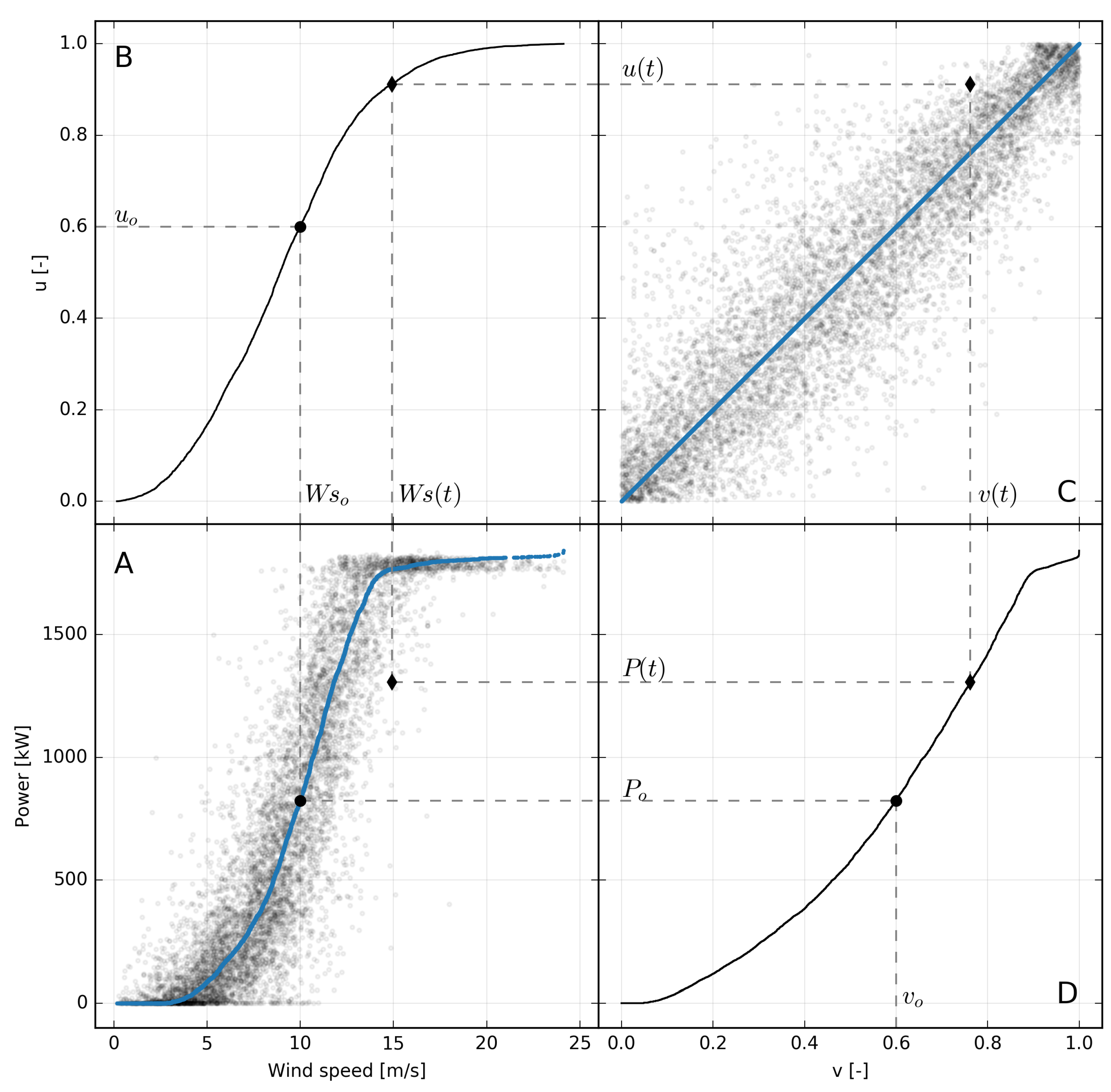
The procedure is illustrated in detail in boxes A, C and D of
Figure 4. Box A shows measured power production against 100 m wind speed forecast for turbine 1. B and D boxes show the quantile
of the cumulative distributions of wind speed and power. In practice,
plots are calculated by sorting the respective time series of
and
P separately and dividing their rank by the total number of samples. In the box A the blue line associates the value of the wind speed for each quantile
to the value of the power in the same quantile:
. This curve correlates wind speed with the power generated by mapping their distributions and constitutes the functional relation for the proposed model.
As a consequence of the independent sorting of the time series needed to calculate the dm curve, the time correspondence between the wind forecast and power measurements is lost. This, which could appear to be a weakness, in practice turns out to be a strong point of the method as it allows, in theory, to apply the same technique also to situations where wind and power are evaluated at different times. For the transformation to make sense, in this case, it is necessary to hypothesize that both data sets are a statistically representative sample of the actual distribution of the two quantities.
A strong argument that can be used to justify the introduction of dm come from its relation with the well known copula method. Copulas have been extensively discussed in literature primarily as a method to characterize the uncertainty of the forecast.
When operating with a sufficiently large sample set, a non parametric copula can be easily generated considering the response curve of the turbine to the wind speed forecast as a bivariate joint distribution
mapping values, evaluated at a given time
t, of wind
and power
into the corresponding quantiles
and
.
Figure 4 illustrates schematically the procedure applied to the wind speed forecast, and corresponding measured power data and the resulting copula shown in box figure D. As it can be seen, the cloud of points, representing wind speed forecasts and corresponding power measurements, in the copula space
, follows the straight line joining (0,0) and (1,1) points. This fact is confirmed by the high value of the correlation coefficient between
u and
v, that in the specific case of
Figure 4 is
.
The more massive concentration of points at the tails reflects the lower correlation between the u and v near the cut-in and the rated powers. Apart from this, the fact that u and v are well linearly correlated is a consequence of a monotonic relationship between wind speed predictions and measured powers. This is also indirectly an indication of the quality of wind speed forecast which, despite being affected by consistent errors, on average has a behavior similar to that which would have the in situ measurements compared to the real power generated by the turbine.
Following these considerations, a reasonable way to choose the "most probable" response curve of the turbine as a function of the wind speed forecast is along the line that bisects the copula space and where the bivariate distribution has its maximum. This line pairs the quantiles of wind speed with the same quantiles of the power production and in the space of physical variables is what we have indicated as dm.
Of course, the choice of dm as response curve to the wind speed forecast doesn’t assure the minimization of any measure of error as it has not been obtained by an optimization algorithm. However, as we will see in the discussion of the results, our method, being obtained from considerations in the space of probabilities shows some interesting characteristics that make it of sure interest due also to its simplicity and immediate applicability.
It is perhaps useful to underline that the quantification of the error obtainable by using the dispersion of points in the space of the copula is only of a statistical nature and not in any way linked to the uncertainty of the specific meteorological forecast. A quantification of the uncertainty “weather-dependent” can only be obtained by using a probabilistic meteorological forecast such as that provided by the ECMWF EPS.
3.3. Benchmark Methods
This technique is compared in the following with a few significant non-parametric methods. The first two benchmark models are based on the so-called Method of Bins. Given a data set of wind speed measurements and the corresponding power values produced by the turbine, the data is divided into wind speed intervals of equal amplitude, typically 0.5 m/s, next, the average wind speed and power output for each bin are calculated. The power curve is obtained by the interpolation of the points. This procedure may be influenced by the presence of outliers in the data. A more robust version of the method can be simply obtained taking the median of the power measurements in the bin instead of the mean. These two methods are identified in the following as mean and median respectively.
The previous methods relate the power output to the value of wind speed at a height level close to the hub height. The result of the NWP is richer than this since it contains information on the wind speed at several levels and the intensity of gusts, for instance. This information may be introduced through machine learning techniques.
A simple data-mining technique is evaluated for comparison, based on the well-known k-nearest-neighbors (kNN) approach [
27]. The features selected to represent the wind conditions at the point of interest are the forecasts of the wind speed 10 m and 100 m above ground and the forecast of the wind gust. This prediction is coupled with a measured power generated by the turbine. Given the NWP forecast, the power prediction is obtained evaluating the k closest points in the feature space from a set of training samples and taking the mean of the associated measured power values. In this case, the parameter k has been chosen by an optimization procedure and is a function of the number of samples in the training set; the method is referred to as
knn in the following.
Artificial Neural Networks (ANN) seem to be the preferred method in the recent literature to predict the power generation by the NWP forecast, a comparison of the proposed methodology with a model based on neural network is therefore necessary. The model is labeled with
ann in the following and is based on a Multilayer Perceptron Model [
18], the input layer takes as input the forecasts of the wind speed at 10 m and 100 m above ground as well as the wind gust. The number and size of the hidden layers and activation function were selected through an optimization procedure, which resulted in a single hidden layer of 5 neurons and a sigmoid activation function.
In both knn and ann, the features and outputs have been scaled to improve the stability.
5. Results and Discussion
First of all the power data available at a frequency of 15 min were filtered, following the indications of the plant operator (see
Figure 2 and discussion in
Section 2), and resampled every 1 h. The NWP data of the 00 UTC analysis time, for forecast times from +25 h to +48 h inclusive were put in line with the recorded power measurements at the same time resolution. This generates a time series of forecasts and corresponding generated power, with a forecast time of at least one day in advance, which cover the whole year 2014.
For the ann and knn models, the wind speeds at 10 m, 100 m and wind gust at 10 m above ground are considered, while for the dm, mean and median models, only the wind speed at 100 m have been used.
The data set for each of the two turbines is divided into a test set and a training set. The train set is filled with some samples taken at random from the complete dataset; the test set consists of all remaining samples. The regression models are trained on the train set, their effectiveness in forecasting is verified on the test set through the error metrics defined in
Section 4.
Different values of the number of samples included in the train set were considered to assess the sensitivity of regression methods to the number of samples of the training set.
The training procedure and the related performance testing is carried out 50 times on randomly taken sets, the results of the reported performances are obtained as an average of the realizations.
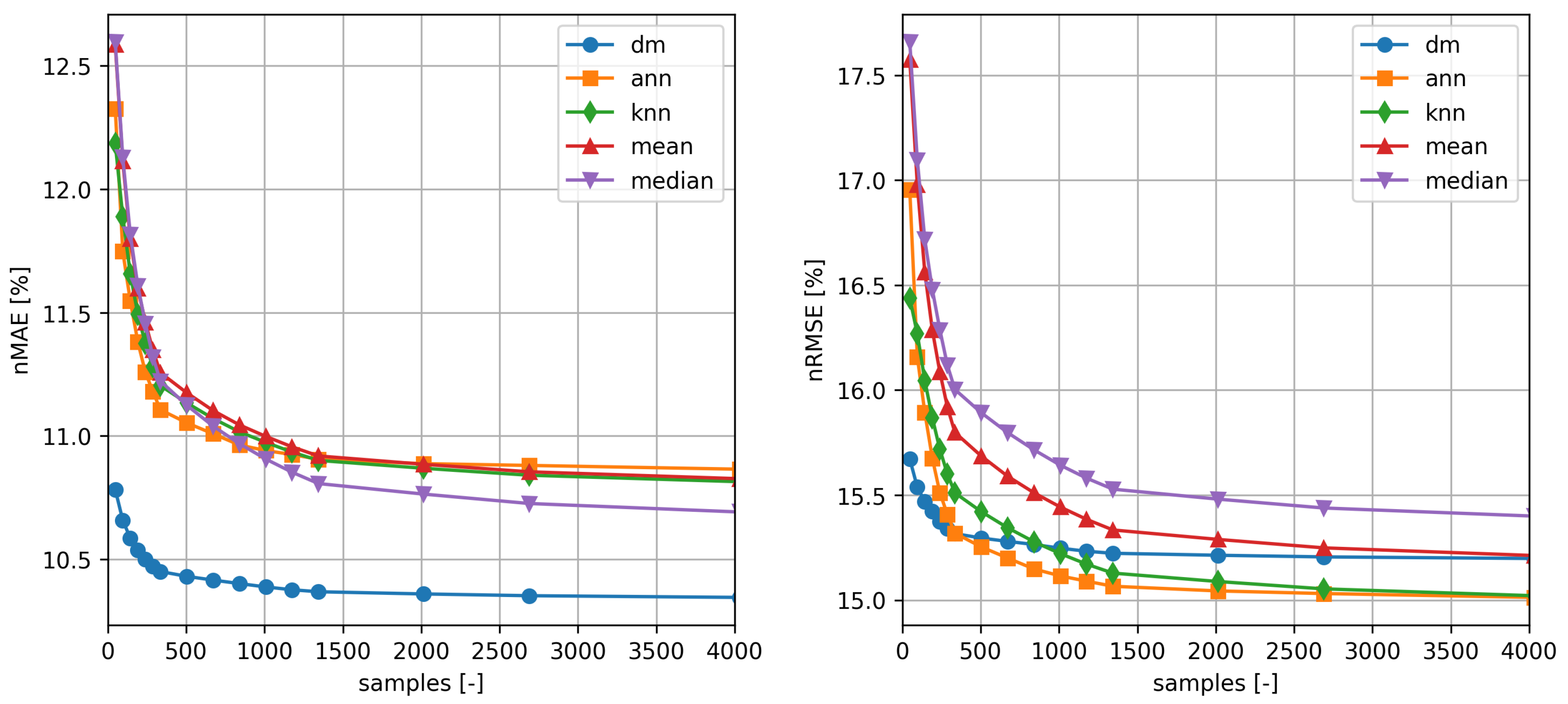
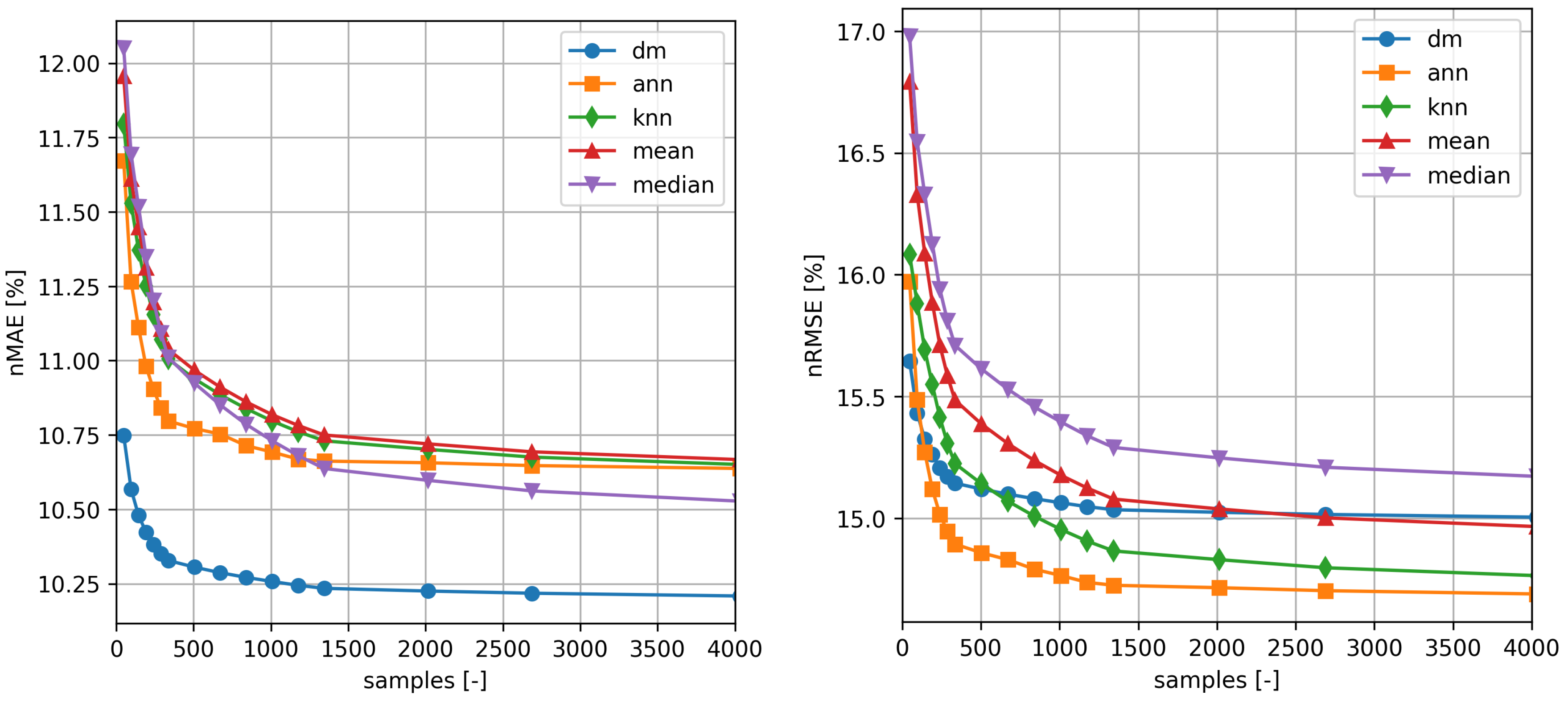
The results for the two turbines for the distribution mapping method and the other methods used as a comparison are shown in the
Table 1 and
Table 2 and in the
Figure 5 and
Figure 6.
As expected, the performance of all methods improves as the number of samples used for training increases. It is also noticeable how the distribution mapping exhibit satisfactory skill even if a dataset with relatively few samples is available. Even the knn and ann methods can be trained with relatively few samples, while Method of Bins models offers satisfactory performance only for larger train sets.
In
Table 1 and
Table 2, the best results for each method, error measure and training time are shown in bold. As it can be seen the performance of the proposed method is not excellent when measured for n
RMSE, while it is considerably better than all the benchmark for n
MAE. Note, also, that the comparison with
ann and
knn methods, it is not completely fair, as the latter by using more features, benefits of additional information about the wind speed profile.
The same kind of information can be extracted from inspection of
Figure 5 and
Figure 6 that show n
MAE and n
RMSE as a function of the number of samples used for training. It is evident that
method performance is better than the maximum that can be obtained with any other method already for a sample of only a couple of hundreds of elements (∼10 days).
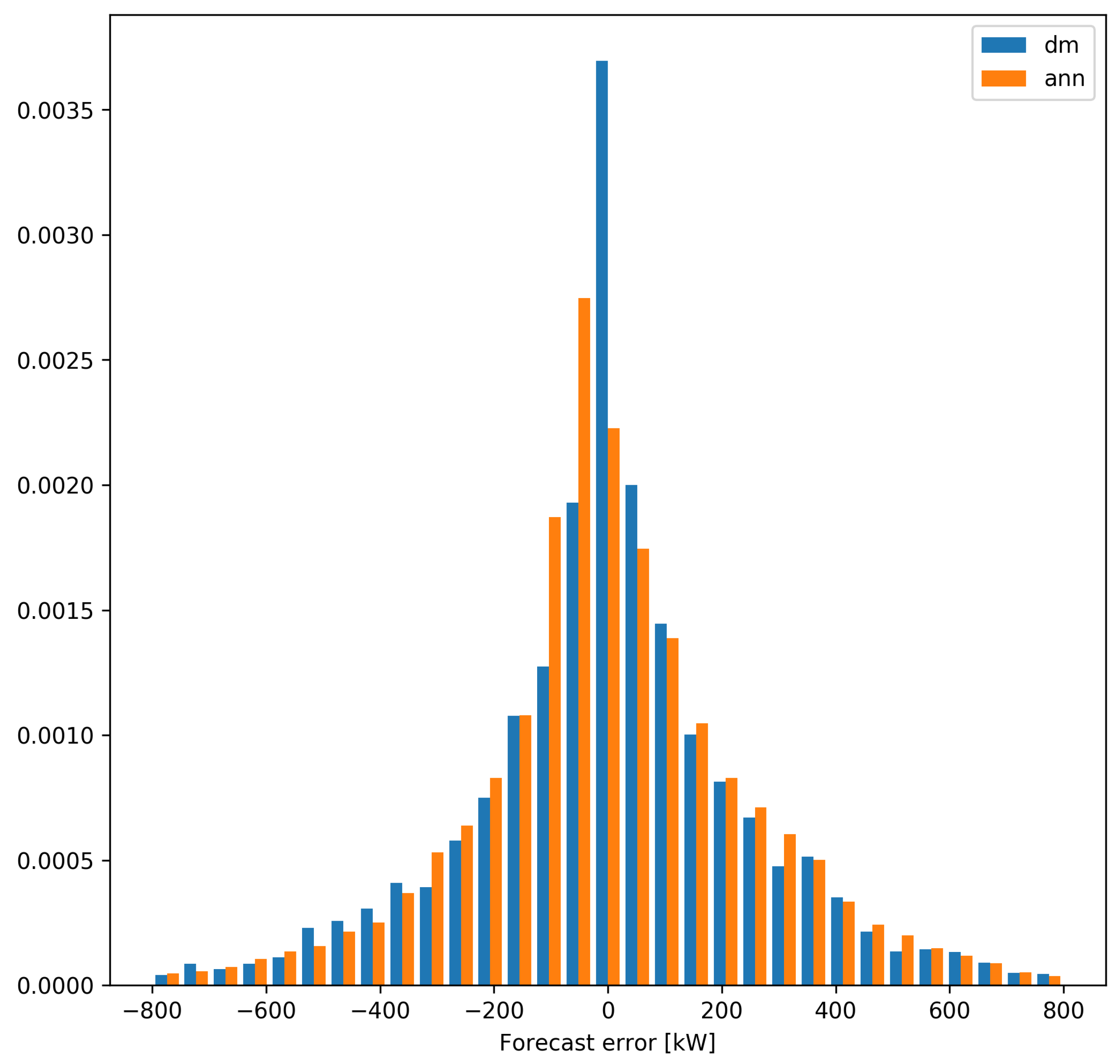
The substantial differences between the forecast errors produced by the
dm and
ann models can also be appreciated in
Figure 7, where the histogram of forecasting errors of turbine 2 is shown. It can be seen that the distribution of errors obtained from the
dm model has a much more marked peak at zero and this behavior is the cause of the smaller size of n
MAE.
As is well known, the n
RMSE measure penalizes large forecasting errors and is preferred in regression procedures for often purely computational reasons, while n
MAE is a flat measure of uncertainty, which can be more practical, sometimes. For example, if the turbine production forecast is used to comply with the manufacturer’s supply contract with the network operator, penalties are paid for errors in the power delivered, and no weight is applied based on the deviation [
28]. Even in a scenario in which the generation error forecast is used as a parameter for the sizing of a storage system serviced to a wind power plant, to guarantee the contracted production profile, the error is, in general, not weighed [
29]. Finally, also the optimal control of a storage system is based on the prediction error without any weight applied to the error itself [
30].
6. Conclusions
This paper introduces a technique for wind power forecasting from meteorological forecast data of wind speeds, which we named distribution mapping (dm), that is suitable for pitch-regulated turbines with a monotonically increasing response curve.
The methodology defines a functional relation between the predicted wind speed and the power, as the transformation between the distribution function of the wind speed and that of the measured power. It has been tested on two turbines installed on the island of Borkum, Germany, within the framework of the European NETfficient project, using the wind speed prediction obtained from the ECMWF model. The accuracy of power forecasting one day in advance and with a resolution of 1 h was assessed and compared with those obtained with other well known methods found in the literature.
The accuracy of the forecasts obtained are remarkable when expressed in terms of MAE, even with respect to the results of much more complex and computationally expensive methods. The method performs well also if a low number of samples is available for its training. Moreover, it can be applied even in unfavorable conditions in which data is fragmentary, asynchronous and with considerable uncertainty (as in the case of the wind forecast used), providing in any case good accuracy.
The aspects of uncertainty, which were overlooked when the deterministic behaviour, that follows from the imposed monotonic trend to the curve dm, was assumed, will be dealt with in a future article using the probabilistic data of the ECMWF ensemble prediction systems (EPS) to quantify the ’weather dependent’ errors of the wind forecast.
Another interesting aspect currently under investigation is the use of the dm curve as a method for the assessment of the operational condition of the wind turbine. The dm technique seem to be appropriate to this purpose due to the short length of the data series needed to calculate it, that therefore can highlight failures of the turbine when a sizable modification of the dm curve is observed.


