A Naive Bayesian Wind Power Interval Prediction Approach Based on Rough Set Attribute Reduction and Weight Optimization

School of Control and Computer Engineering, North China Electric Power University, Beijing 102206, China
*
Author to whom correspondence should be addressed.
Energies 2017, 10(11), 1903; https://doi.org/10.3390/en10111903
Submission received: 19 October 2017
/
Revised: 13 November 2017
/
Accepted: 15 November 2017
/
Published: 19 November 2017
(This article belongs to the Special Issue Wind Generators Modelling and Control)
Abstract
:Intermittency and uncertainty pose great challenges to the large-scale integration of wind power, so research on the probabilistic interval forecasting of wind power is becoming more and more important for power system planning and operation. In this paper, a Naive Bayesian wind power prediction interval model, combining rough set (RS) theory and particle swarm optimization (PSO), is proposed to further improve wind power prediction performance. First, in the designed prediction interval model, the input variables are identified based on attribute significance using rough set theory. Next, the Naive Bayesian Classifier (NBC) is established to obtain the prediction power class. Finally, the upper and lower output weights of NBC are optimized segmentally by PSO, and are used to calculate the upper and lower bounds of the optimal prediction intervals. The superiority of the proposed approach is demonstrated by comparison with a Naive Bayesian model with fixed output weight, and a rough set-Naive Bayesian model with fixed output weight. It is shown that the proposed rough set-Naive Bayesian-particle swarm optimization method has higher coverage of the probabilistic prediction intervals and a narrower average bandwidth under different confidence levels.
1. Introduction
Wind power generation has become one of the most popular renewable energy sources in the world due to its clean energy and wide availability. However, because of the intermittent and fluctuating nature of wind power generation, relying on wind for the safe and stable operation of a power grid is challenging [1]. In order to solve this problem, it is very important to predict the wind power more effectively [2,3]. A lot of physical and statistical prediction methods have been put forward in recent years. The physical models use numerical weather prediction (NWP) to predict wind speed and then input the data into wind power output models to obtain the output power [4]. The common statistical forecast methods include the time series method [5,6], artificial neural network (ANN) method [7,8], and support vector machine (SVM) [9]. The main focus of these methods is to reduce the point forecast errors of wind power by introducing new models. In [10], the original wind power data are decomposed by Ensemble Empirical Mode Decomposition (EEMD) and the decomposition sequences that are reduced by the principal component analysis are predicted by the least squares support vector machine. However, prediction errors cannot be fully eliminated, even if the best forecasting tools are adopted [11]. Epistemic uncertainty errors originate from incomplete knowledge about the stochastic characteristics and heavy fluctuation of wind speed, and from the nonlinear relationship between wind speed and wind power. As a result, probabilistic interval forecasting to provide uncertainty information for wind power [12] has gotten much attention in recent research.
Probabilistic interval forecasting tries to predict a range of potential output power comprising a lower and upper bounder under a given confidence level, and clarify uncertain information in a wind power forecast. Decision makers can analyze this information to make better decisions to plan and operate a power grid safely. In recent years, significant probabilistic forecasting research has been carried out. The conventional methods of a probabilistic forecast often require some special prior assumptions of error distribution of point prediction [13]. It is not reasonable to assume a specific point error distribution such as Gaussian or Beta for any wind farm. In [14], the probability intervals of the uncertain power output of wind power are established by analyzing the error distribution characteristics of the studied case. In [15], after conversion of multivariate Gaussian random variable by using prediction errors generated in a series, a statistical method for efficient wind power prediction is established. However, these methods have heavy computation requirements and are unattractive for real applications. The advantages of the alternate methods for determining probabilistic wind power prediction intervals (PIs), such as the kernel density forecast method [16,17] and quantile regression [18,19], include the lack of specific assumptions about error distribution. However, the forecasting accuracy of these methods depends on the point forecasting value, so if the accuracy of point forecasting is very weak, then the prediction intervals will have poor performance. Without prior knowledge of point forecasting, some intelligent models have been employed to generate probability intervals. The authors of [20] reported a wind power prediction system that is trained using ANN, in which the optimal choice of hidden neuron is chosen by a heuristic method. In [21], the prediction model is established through a kernel extreme learning machine (KELM). One key issue for these methods is how to select reasonable trained data to obtain a high-precision intelligent model that approximates the nonlinear relationship between the input and output variables. The existing researches have obtained wind power prediction intervals by either analyzing the error characteristics of point prediction or using intelligent model, however they are commonly lacking the consideration about probabilistic information of wind speed or power data in historic operation data.
The Naive Bayesian method provides a probabilistic means of reasoning. It assumes that the variables to be tested comply with some probability distribution. Inferences can be further done based on these probabilities and the observed data, and then optimal decisions can be achieved. In [22], a Bayesian estimation of remaining useful life is implemented for wind turbine blades. In this paper, by making use of the prior knowledge of data and priori probability, a probabilistic interval forecasting model is constructed based on Naive Bayesian theory. As is known, identifying significant input variables is critical when constructing an accurate prediction model. Rough set (RS) theory can be utilized to deal with data-sets with poor information and to remove irrelevant attributes from a data-set [23]. So, in our designed model, RS is employed to use to select significant variables as input variables for the Naive Bayesian prediction interval model. A Naive Bayesian classifier is established to predict the power class. Particle Swarm Optimization (PSO) algorithm is a random search and parallel optimization, and it can easily search the global optimal solution. In [24], PSO are used to produce an optimal weight strategy for weighted evaluation indexes. In order to improve the accuracy of the prediction intervals, a PSO algorithm, which is based on an objective function, is employed to optimize the output weight of Naive Bayesian predictive power, in order to calculate reasonable lower and upper bounders.
The rest of this paper is organized as follows. In Section 2, the overall structure and basic theoretical knowledge of the proposed approach are described. The construction step of the Rough Set-Particle Swarm Optimization-Naive Bayesian (RS-PSO-NBC) wind power intervals model is presented in Section 3, and the simulation results of the proposed approach, which are compared with other methods, are presented in Section 4. Finally, conclusions are given in Section 5.
2. Proposed Approach for Forecasting Wind Power Intervals and General theory
The structure of the proposed prediction intervals model is shown in Figure 1.
In the prediction model, represents the relevant input variables used to predict model learning, and is the Naive Bayesian classifier input for the model whose attributes are roughly reduced by rough sets. and are the upper and lower bounds of the wind power prediction intervals, respectively, and is the output weight of the Naive Bayesian Classifier, named and . In order to improve the prediction accuracy, the optimal value of (including and ) is determined by particle swarm optimization.
2.1. Basic Theory of Rough Sets
Rough set theory [25,26] is a data analysis theory proposed by academician Z. Pawlak of the Poland Academy of Sciences. It mainly deals with information systems that are characterized by inexact, uncertain, or vague information. One advantage is that rough set theory does not need any preliminary or additional information about the data. It can effectively process data and information in complex systems, and it can analyze and reason data. It has been widely used in data mining, decision analysis, pattern recognition, and so on.
The basic object of a rough set is a knowledge system. In rough set theory, the expression of a knowledge system is:
In this formula, is the domain; is a set of attributes, where is the condition attributes of the decision attribute and is the decision attribute. is the collection of attribute values, and is the value range of the attribute value ; is information system. A knowledge expression system that has both conditional attributes and decision attributes is often referred to as a decision system. The decision system is represented by a decision table, the rows of the decision table represent the elements of the domain, and the columns represent different attributes.
Let be a condition attribute of the decision system. In rough set theory, the dependency degree of condition attribute to decision attribute is defined as:
In the formula, is the positive domain of the knowledge of the decision attribute , which is the set of objects in the domain . This domain can be accurately divided into the equivalence classes of the relational according to the classified information; is the number of elements in a domain. represents the proportion of objects that can be accurately assigned to the decision class under the condition attribute , and describes the extent to which the conditional attribute supports the decision attribute .
For a decision system, every condition attribute has a different degree of dependency to the decision attribute , and the dependency degree of the conditional attributes to the decision attributes is called the significance of the conditional attributes. In rough set theory, after removing the condition attribute, the significance of the condition attribute is evaluated by the change of the classification ability of the decision system.
The significance of is expressed as :
Larger values for show that in the condition attributes of set , the greater the impact of conditional attribute on decision-making, the more important the conditional attribute is; conversely, the smaller impact the conditional attribute has on decision-making, the less important the conditional attribute is, or it may even be the result of an error.
The selection of the input variables for the Naive Bayesian Classifier will affect the prediction accuracy. Since the rough set does not need any a priori information, only data analysis, the objective significance of each condition attribute, can be obtained. Therefore, we employ rough set theory to identify significant conditional attributes as the input of the Naive Bayesian.
2.2. Naive Bayesian Classifier
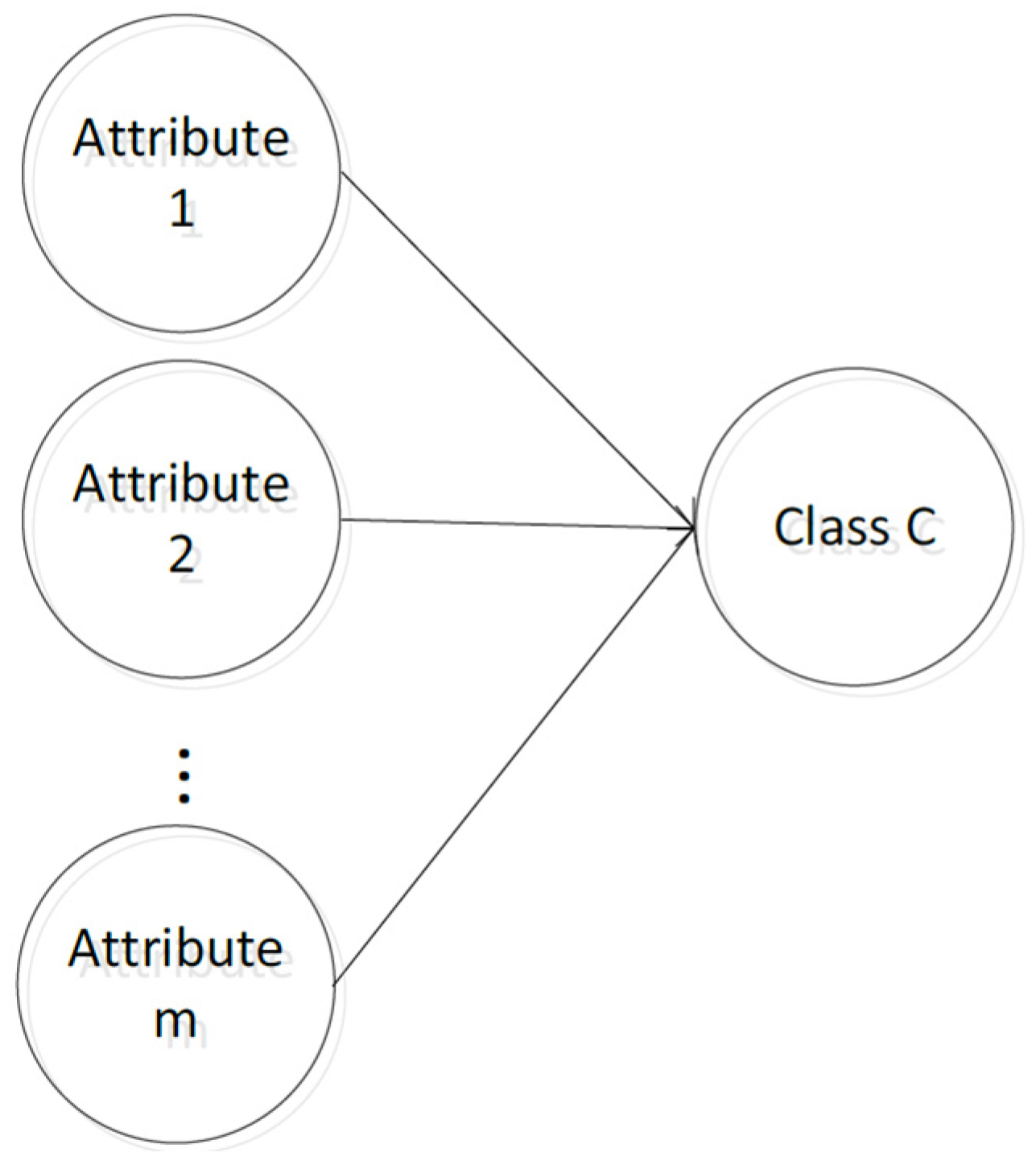
A Naive Bayesian Classifier (NBC) is one of the most widely used models among Bayesian Classifiers [27,28]. The Naive Bayesian Classifier model is shown in Figure 2:
Suppose a set of variables , where includes conditional attributes. , containing class labels. The Naive Bayesian Classifier model assumes that the conditional attributes are all child nodes of the class variable . Assign a given sample to be assigned to class and only if: .
According to Bayes’ theorem, there are:
where is the unconditional probability (also known as the priori probability) of the sample to be sorted, and is the conditional probability (also called posterior probability) that is given for the category in the case of a given class .
If you do not know the probability of the data set in advance, you can assume that the probability of each category is equal. Use this to maximize :
Otherwise, maximize . Since is constant for all of the categories,
By the Naive Bayesian Classifier algorithm, the conditional properties are independent of each other:
where , is the number of instances of class in the training sample, and is the total number of training samples. Thus, the NBC model formula expression is:
The probability of can be estimated by the training sample. By this formula, the sample to be classified is of the class .
2.3. The PSO Algorithm
PSO is a kind of evolutionary computation technique that is based on swarm intelligence, simulating the migration and clustering behavior in the process of birds foraging, and was proposed in 1995 by Kennedy and Eberhart [29]. In PSO, each solution to an optimization problem is a bird in the search space, called a “particle”. Each particle has an initialization speed and position, and an adaptive value is determined by the fitness function. All of the particles have a memory function so that they can remember the best location that has been searched, and each particle has a speed that determines the direction and distance that they fly, so that particles can search the solution space in the optimal particle.
In the process of each iteration, the two most important operators of PSO are velocity and position update. By comparing the fitness value and two extreme values, we can finally find the individual optimal solution (pbest) and global optimal solution (gbest). The classic formulas for velocity and position update are shown below:
where is the number of iterations and is the inertia weight. is represented as the position velocity of the ith particle. are two positive constants. are uniformly distributed random numbers. is the history of the individual optimal location of the ith particle, and is the population’s optimal location.
With a random search and parallel optimization, PSO algorithm has proven its simplicity, robustness, ease of implementation, and rapid convergence. It can easily find the global optimal solution of a problem. Therefore, in this paper, we chose the PSO algorithm to optimize the output weight , satisfying the objective function minimization. According to the optimization criteria of PSO, we get the model’s best output , which will be used to obtain the optimal PIs in the future.
3. Establishing the RS-PSO-NBC Wind Power Intervals Model
Probabilistic interval forecasting is composed of an upper and lower boundary with a certain probability level. As shown in Figure 1, this paper constructs an upper and lower bound estimation model of RS-PSO-NBC. After the original input, was put into a rough set to remove irrelevant attributes, the significant inputs identified by RS are used as conditional attributes for the NBC. The NBC uses the data distribution hypothesis and prior knowledge to classify power into a reasonable class. Then, the dual output bounds of upper and lower for the wind power are calculated with optimized weight (the upper-weight and the lower-weight ) by PSO. The detailed prediction process is described below.
3.1. Rough Set Selects Criteria Attribute
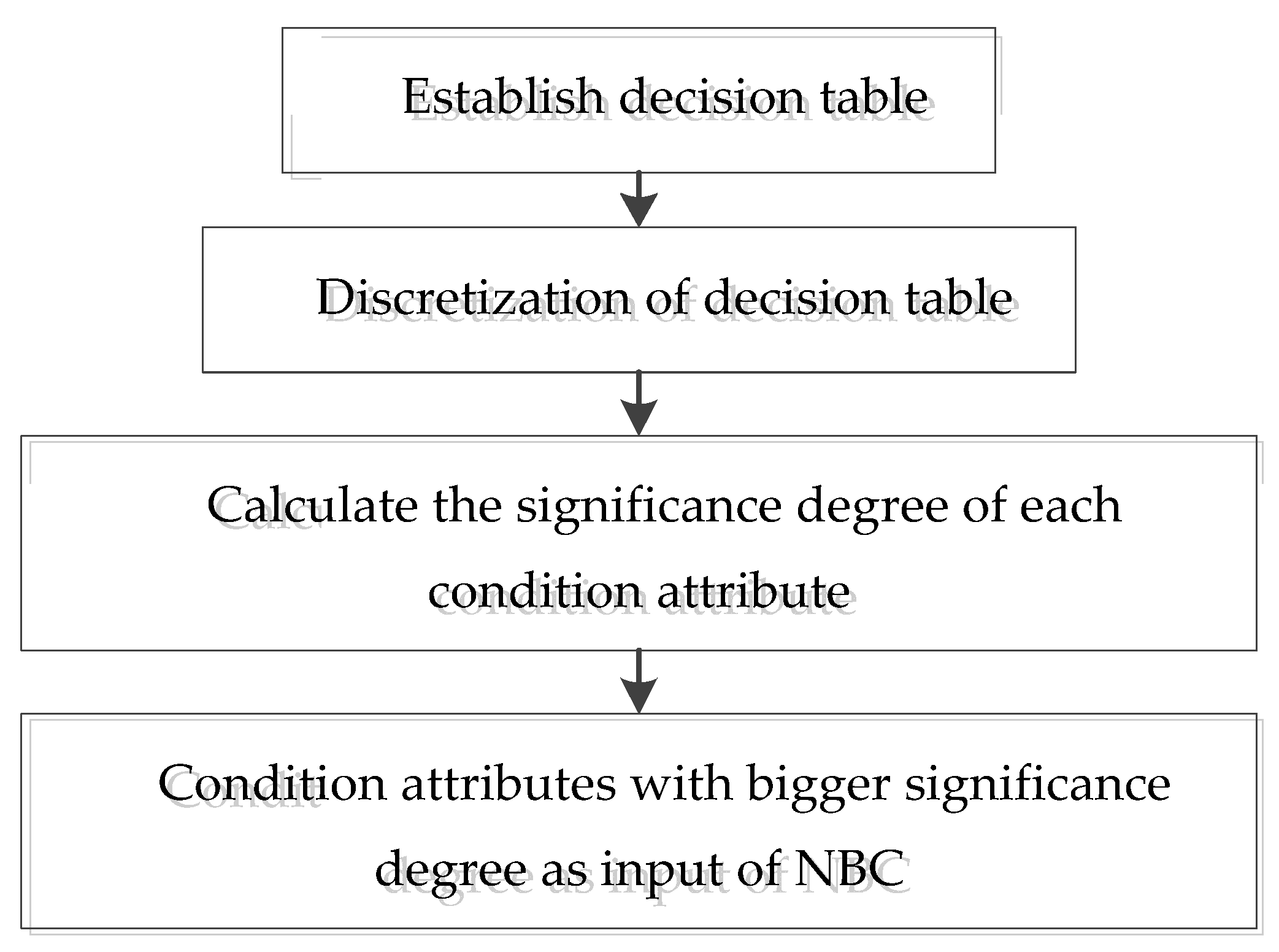
The rough set is employed to identify the significant condition attribute as an input of NBC. A flowchart of the reduced condition attributes is shown as Figure 3.
The decision process is as follows:
- (1)
- Establish a decision table. For a sample , the wind speed ; ; , the power of ; ; ; and are taken as original condition attributes, , . Wind power output is selected as the decision attribute . One element of universe can be defined as ,
- (2)
- Discretize the decision tables. Rough sets can only deal with discrete information, so the decision table needs to be discretized. In this paper, an equidistant interval algorithm is used. According to the maximum and minimum values for wind power, the value interval of is divided into 20 discrete intervals, and the values falling in each interval are equal to 1, 2, 3, ..., 20 respectively. is also discretized according to the maximum and minimum values of the wind speed.
- (3)
- Calculate the attribute significance of each condition attribute and determine the input for NBC.
According to Formula (3), the significance degree of each condition attribute is calculated, and the appropriate condition attribute is selected according to the significance degree as the input of the NBC prediction model.
3.2. The Naive Bayesian Classifer Infers the Power Class
A Naive Bayesian classifier firstly uses the condition attribute that is selected by rough sets as the input vector, and then uses the preliminary knowledge and distribution of data to process known data. Finally, the inference and analysis are implemented according to the prior probability distribution of data, and an optimal decision about the predictive power class is made.
3.3. PSO Optimizes Output Weight
Because wind power varies widely from zero to rated power during operational conditions, if only one optimum weight in the prediction model is used for the whole of the wind power, it will reduce the accuracy of the prediction intervals. We adopt the model to optimize weight individually in specified ranges of wind power, to improve accuracy. In other words, we divided wind power into n power intervals. Applying the particle swarm optimization algorithm, a different optimum weight could be found for every power interval. The equal interval method is used to divide the power interval. The power range is , and assuming that the power interval length is , then the partition is:
For , is the number of sections.
3.3.1. Optimizing the Objective Function
The accuracy of the prediction intervals model can be evaluated in terms of reliability and accuracy. Reliability indicates the probability of actual observations falling into PIs, so it should be as large as possible. The PI width expresses sharpness. This value should be as small as possible, so that the predicted widths are as narrow as possible. However, the two indices are contradictory. In this paper, we construct a comprehensive optimization objective function F, as follows:
where and are the weights of PINE, PINAW. is the absolute value for PICE, PINAW. PICE = |PINC-PICP|, PINC is the Confidence level. The PICP reflects the probability that the target value falls within the upper and lower bounds of the predicted intervals:
where is the number of predicted samples. is the Boolean quantity, and if the predicted target value is included in the upper and lower bounds of the intervals prediction, then ; otherwise . For an effective prediction interval, PICP should be close to PINC.
PINAW is the predicted intervals’ average bandwidth, and to some extent can reflect sharpness. If PINAW is too wide, it cannot give an effective predictive information of uncertainty:
Adjusting the weight factor can control the ratio of different criteria’s influence on the optimization results.
3.3.2. Weight optimization by PSO
Using the objective function F shown in (13) as a fitness function, and taking a power partition as an example, the steps for weight optimization by PSO are as follows:
- (1)
- Initialize the particle swarm, via random initialization of the particles.
- (2)
- Calculate the fitness of each particle according to the objective function F, as shown in (13).
- (3)
- For each particle, its fitness is compared with its historical optimum fitness, and if the current fitness is better, that fitness is denoted as the historical optimum value.
- (4)
- For each particle, compare its fitness and the fitness of the best position experienced by the swarm; if better, it is optimal as a swarm.
- (5)
- The velocity and position of the particle are evolved according to the velocity and position update Equations (9)–(10).
- (6)
- If the end condition is reached (an optimal solution or the maximum number of iterations), then the swarm optimal position is the optimal output weight , otherwise go to step (2).
3.4. The Prediction Process
A flowchart of the proposed strategy for forecasting wind power intervals is illustrated in Figure 4.
The detailed steps are as follows:
- (1)
- Firstly, the rough set is used to reduce the input variables, and the selected condition attribute is taken as the input for the NBC interval prediction model. The data is pre-processed. The data is divided into a training data set and test data set. Training data output (wind power) fluctuates up and down slightly, as the upper and lower bounds for the initial prediction model to determine the initial output weight .
- (2)
- The conditional attribute selected by the rough set is taken as the input of the Naive Bayesian, and the Naive Bayesian model is established by using training data.
- (3)
- Initialization parameters of PSO are established, including set population and iteration, initial particles position around , random initial velocity, and individual and global optimum position.
- (4)
- The wind power is divided into power partitions with equal intervals, and the different power segments are optimized by particle swarm to find the respective optimum values of output weight. The fitness, the speed, the position, and the global optimal value of each particle are calculated according to relative equations in each iteration. After the iteration, the optimal output weight obtained.
- (5)
- Applying the trained Naive Bayesian prediction intervals to the test data, the output result of the wind prediction intervals is calculated, and the PIs are evaluated by the evaluation index.
4. Simulation Results and Analysis
In our simulation, the proposed prediction model is tested using the wind power data from a wind farm in Gansu province, Northwest China. The total installed capacity is 199.5 MW. There are 100 wind turbines in wind farm and the rated power for wind turbine is 2 MW. The data was recorded in 15 min intervals. A numerical weather prediction (NWP), including wind speed, was also recorded. Taking the data of three months as an example, the data was divided into a training set and a testing set. The feasibility of this method is verified by simulation, and the results are compared with the Naive Bayesian method and the rough set Naive Bayesian method to verify the superiority of the new method.
4.1. Significant Condition Attributes Reduced by Rough Set
According to the procedure described in Section 3.1 using the trained data, the predicted wind speed of numerical weather ; ; the power of ; ; ; are taken as the condition attribute , the true value of the wind power output is taken as the decision attribute , and the decision table is established and discretized as shown in Table 1.
The discrete decision table is processed, and according to Formula (3), the attribute significance is calculated, as shown in Table 2.
It can be seen from Table 2 that the significance degrees of variables ; are relatively smaller. Thus, we can choose the input variables of ; ; or ; ; ; ; as the inputs of the Naive Bayesian interval prediction model. The simulations have been done for different input variables under confidence levels 90%. The results indicated that the PICP(Prediction Intervals Coverage Probability) = 90.03% and PINAW(Prediction Intervals Normalized Average Width) = 194.2064 were obtained under case of three input variables. The PICP = 89.7% and PINAW = 229.4473 were achieved under case of five input variables. The reason is probably that the power data and have already been embedded with wind speed information and , and due to the increasing of the input variables, the Naive Bayesian prediction model will increase the complexity and reduce the accuracy of the results. So, the wind speed and power ; are determined as the input variables.
4.2. Results of Predictive Intervals
The operation of a power system always requires a higher level of confidence in order to obtain more accurate information, so the confidence levels were chosen to be 80%, 85%, and 90%. Let , . The power interval is . The PSO population size was set to 80, and the initial position of the particle was calculated by the initial output weight, with particle velocity as a random number from 0 to 1. Particle dimension was chosen for the output weight dimension. The fitness value of each particle is calculated in accordance with the optimization criterion F given above, during each iteration. The inertia weight is an important parameter of the PSO algorithm, because a larger inertia weight can enhance the ability of a global search, while a smaller inertia weight will enhance the local search ability of the algorithm. This article uses the dynamic adjustment of inertia weight strategy, and the dynamic adjustment with linearly decreasing inertia weight strategy:
where , , , is the number of iterations, to the current number of iterations.
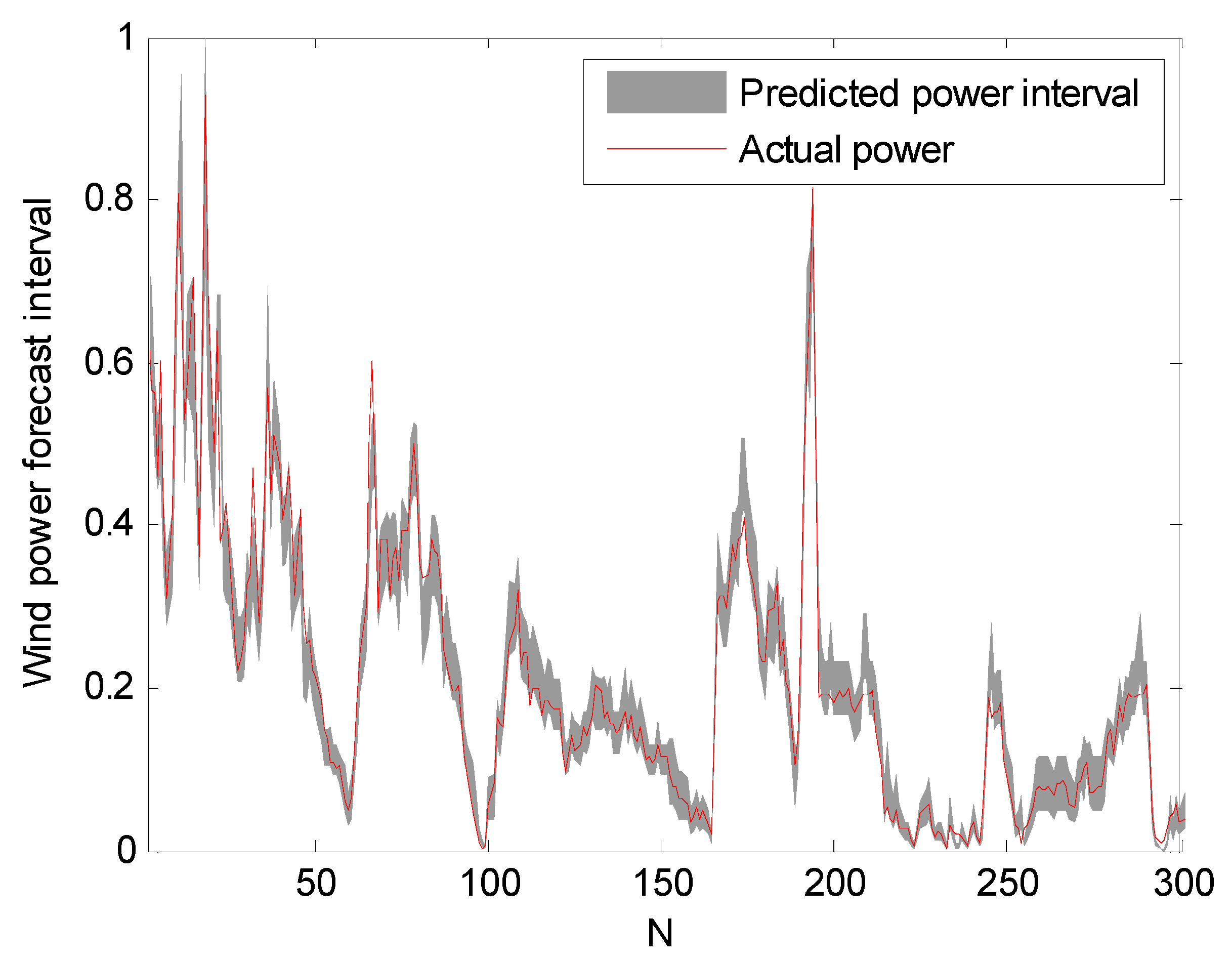
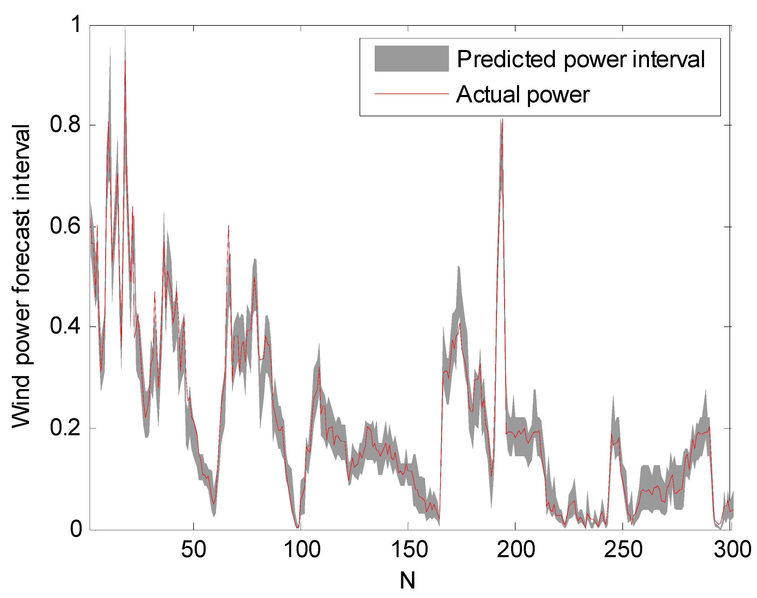
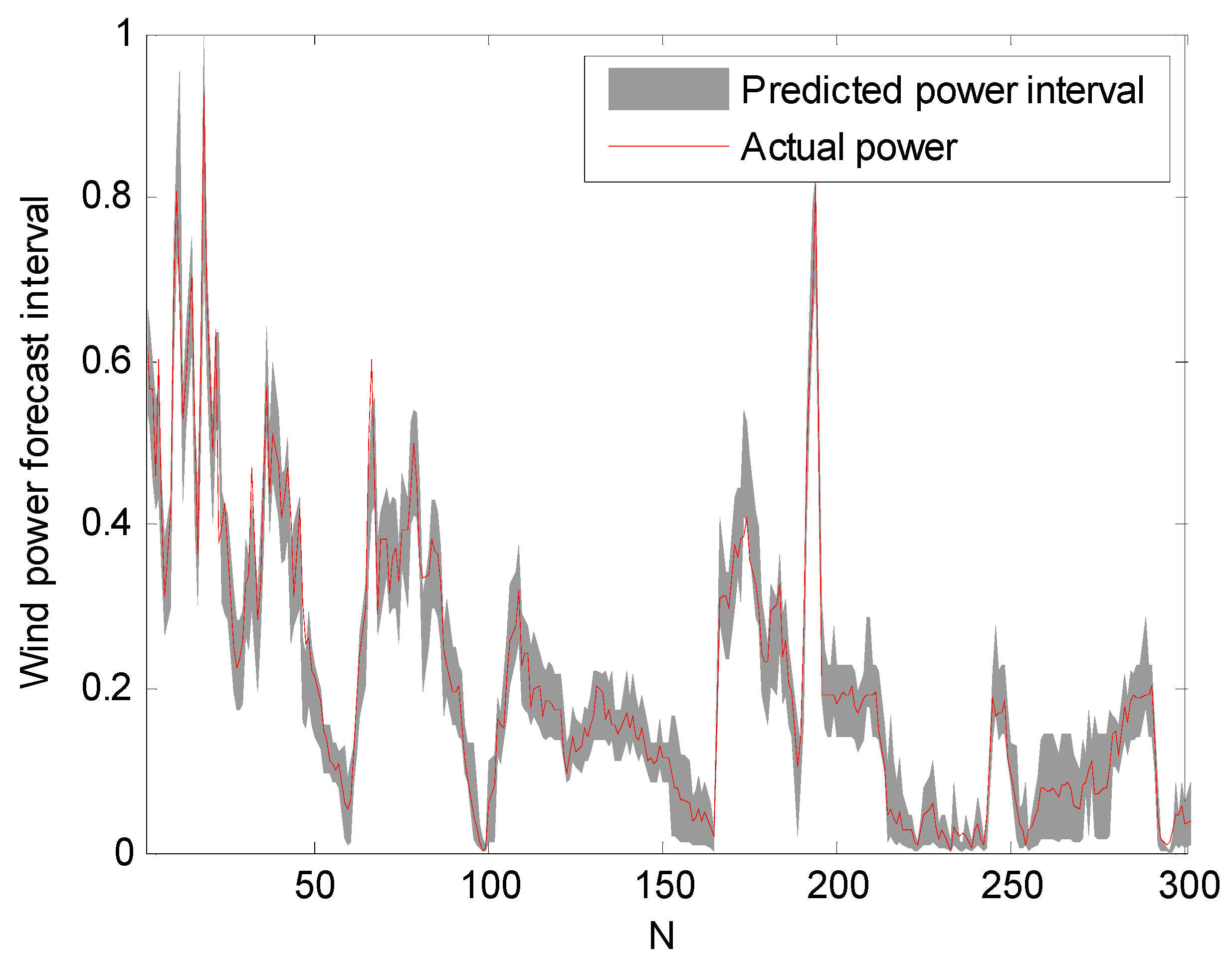
The prediction intervals at confidence levels 80%, 85%, and 90% are shown in Figure 5, Figure 6 and Figure 7. For clarity, only a portion of the data (the first 300 points) are shown.
It can be seen from Figure 5, Figure 6 and Figure 7 that the proposed approach is effective and most of the real values are within the prediction intervals. The RS-PSO-NBC model can maintain both the reliability and the accuracy for the index. Also, the width of the confidence interval increases as the confidence level increases, since the wider the confidence interval, the higher probability that the predicted intervals contain the actual power value, which is consistent with the theoretical knowledge.
4.3. Results of Optimizing Weights for Each Power Segment by PSO
Table 3 shows the output weights for each power segment corresponding to the Naive Bayesian prediction model by PSO, at the 85% confidence level. It can be seen from Table 3 that the optimal output weights of the individual power partitions are different, so the optimal output weights of the respective power segments should be used to improve the accuracy of the prediction intervals.
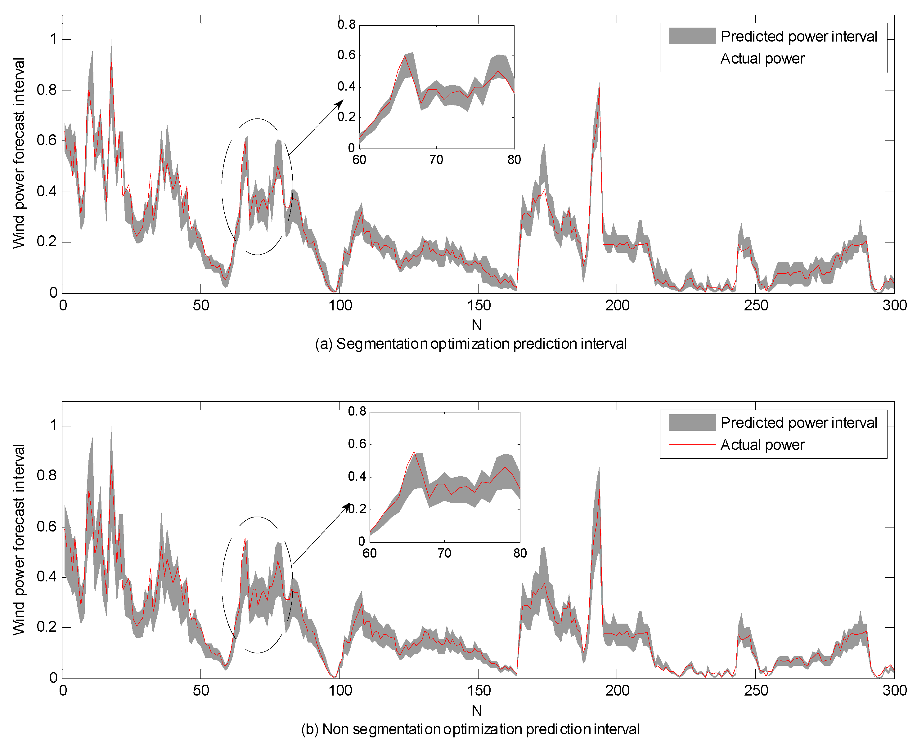
In order to verify the effect of segment optimization, a comparison with non-segmented optimization weight (using one optimal weight for the whole power district via PSO) was also carried out. It can be seen from Figure 8 that the proposed segmented optimization model can ensure the tracking intervals of the wind power time series, accompanied with a narrower upper and lower bound. This can provide better uncertainty information for decision makers.
4.4. Comparison with Other Methods
In order to further demonstrate the superiority of the interval prediction method as proposed in this paper, the results of the approach that only uses the Naive Bayesian method are examined. The original five variables are taken as the inputs of the Naive Bayesian model, the weight is assigned 1.26, and the weight is assigned 0.8. Simulation results are shown in Table 4. Furthermore, in order to verify the effectiveness of optimal weight by PSO, the results of the approach based on the rough set and Naive Bayesian model (RS-NBC) (where three input variables reduced by RS are employed, the weight is assigned 1.19, and the weight is assigned 0.722, are also shown in Table 4. In Table 4, RS-PSO-NBC is the proposed model, NBC is the Naive Bayesian method, and RS-NBC is the rough set and Naive Bayesian model.
It can be seen from Table 4 that in terms of the reliability index PICP (the bigger the better), at each confidence level the proposed model values are the biggest. The PICP values of the proposed approach are 80.87%, 85.51%, and 90.45% at confidence levels 80%, 85%, and 90%. At the same time, under these three confidence levels, the PICP values of the NBC approach are 79.56%, 84.84%, and 89.67%, which indicates that the predicted power value does not fall within the predicted intervals at the set confidence level. Therefore, the NBC method loses predictive reliability. In terms of the accuracy index PINAW (the smaller the better), the average bandwidth values of the proposed method are the smallest: 190.2462, 228.8533, and 271.6239 at confidence levels 80%, 85%, and 90%. That is to say, the proposed method can achieve higher prediction performance due to combining rough set theory with Particle Swarm Optimization.
5. Conclusions
The method proposed in this paper for Naive Bayesian wind power probability interval prediction, featuring particle swarm optimization and rough set condition attribute selection, has the following characteristics:
- (1)
- The Naive Bayesian method is used to obtain the output power probability intervals, making use of the prior knowledge and distribution hypothesis of known data, and to reason from the observed data according to these probabilities and distributions to make the optimal judgment.
- (2)
- Rough set theory is used to reduce the inputs of the Naive Bayesian prediction model and to improve input selection accuracy, which improves the accuracy of the wind power prediction intervals.
- (3)
- Different power segments have different characteristics, and the output weights of the Naive Bayesian Classifier prediction model for these power segments are also different. Using the particle swarm optimization algorithm to find the optimal power output weights, respectively, higher coverage and narrower average bandwidth for the wind power forecasting intervals can be obtained.
- (4)
- In this paper, we use two evaluation indices: the predicted interval coverage probability and the average bandwidth of the intervals. The interval coverage probability indicates reliability, and the average bandwidth can be used to evaluate the interval coverage probability on the basis of their accuracy. Finally, a comparison between NBC and RS-NBC shows the superior interval prediction of the proposed approach.
Acknowledgments
The authors would like to acknowledgment to the funding support from National Nature Science Fund Project (51677067), the Fundamental Research Funds for the Central Universities (2015MS24).
Author Contributions
Xiyun Yang conceived and designed the algorithm; Feng Gao organized and processed the data; Guo Fu performed the experiments; Yanfeng Zhang and Ning Kang analyzed the results. All authors approved the manuscript.
Conflicts of Interest
The authors declare no conflict of interest.
References
- Miller, N.W.; Guru, D.; Clark, K. Wind generation. IEEE Ind. Appl. Mag. 2009, 15, 54–61. [Google Scholar] [CrossRef]
- Khosravi, A.; Nahavandi, S. Combined nonparametric prediction intervals for wind power generation. IEEE Trans. Sustain. Energy 2013, 4, 849–856. [Google Scholar] [CrossRef]
- Shi, J.; Guo, J.; Zheng, S. Evaluation of hybrid forecasting approaches for wind speed and power generation time series. Renew. Sustain. Energy Rev. 2012, 16, 3471–3480. [Google Scholar] [CrossRef]
- Chen, N.; Qian, Z.; Nabney, I.T.; Meng, X. Wind Power Forecasts Using Gaussian Processes and Numerical Weather Prediction. IEEE Trans. Power Syst. 2014, 29, 656–665. [Google Scholar] [CrossRef]
- Liu, H.; Erdem, E.; Shi, J. Comprehensive evaluation of ARMA-GARCH(-H) approaches for modeling the mean and volatility of wind speed. Appl. Energy 2011, 88, 724–732. [Google Scholar] [CrossRef]
- Kavasseri, R.G.; Seetharaman, K. Day-ahead wind speed forecasting using f-ARIMA models. Renew. Energy 2009, 34, 1388–1393. [Google Scholar] [CrossRef]
- Li, G.; Shi, J. On comparing three artificial neural networks for wind speed forecasting. Appl. Energy 2010, 87, 2313–2320. [Google Scholar] [CrossRef]
- Hong, Y.Y.; Chang, H.L.; Chiu, C.S. Hour-ahead wind power and speed forecasting using simultaneous perturbation stochastic approximation (SPSA) algorithm and neural network with fuzzy inputs. Energy 2010, 35, 3870–3876. [Google Scholar] [CrossRef]
- Zhou, J.; Shi, J.; Li, G. Fine tuning support vector machines for short-term wind speed forecasting. Energy Convers. Manag. 2011, 52, 1990–1998. [Google Scholar] [CrossRef]
- Wu, Q.; Peng, C. Wind power generation forecasting using least squares support vector machine combined with ensemble empirical mode decomposition, principal component analysis and a bat algorithm. Energies 2016, 9, 261. [Google Scholar] [CrossRef]
- Bremnes, J.B. A comparison of a few statistical models for making quantile wind power forecasts. Wind Energy 2006, 9, 3–11. [Google Scholar] [CrossRef]
- Pinson, P.; Nielsen, H.A.; Moller, J.K.; Madsen, H.; Kariniotakis, G.N. Non-parametric probabilistic forecasts of wind power: Required properties and evaluation. Wind Energy 2007, 10, 497–516. [Google Scholar] [CrossRef]
- Zhang, G.; Wu, Y.; Wong, K.P.; Xu, Z.; Dong, Z.Y.; Iu, H.H. An advanced approach for construction of optimal wind power prediction intervals. IEEE Trans. Power Syst. 2015, 30, 2706–2715. [Google Scholar] [CrossRef]
- Tewari, S.; Geyer, C.J.; Mohan, N. A statistical model for wind power forecast error and its application to the estimation of penalties in liberalized markets. IEEE Trans. Power Syst. 2011, 26, 2031–2039. [Google Scholar] [CrossRef]
- Pinson, P.; Madsen, H.; Nielsen, H.A.; Papaefthymiou, G.; Klockl, B. From probabilistic forecasts to statistical scenarios of short-term wind power production. Wind Energy 2009, 12, 51–62. [Google Scholar] [CrossRef] [Green Version]
- Bessa, R.J.; Miranda, V.; Botterud, A.; Zhou, Z.; Wang, J. Time-adaptive quantile-copula for wind power probabilistic forecasting. Renew. Energy 2012, 40, 29–39. [Google Scholar] [CrossRef]
- Taylor, J.W.; Jeon, J. Forecasting wind power quantiles using conditional kernel estimation. Renew. Energy 2015, 80, 370–379. [Google Scholar] [CrossRef] [Green Version]
- Haque, A.U.; Nehrir, M.H.; Mandal, P. A hybrid intelligent model for deterministic and quantile regression approach for probabilistic wind power forecasting. IEEE Trans. Power Syst. 2014, 29, 1663–1672. [Google Scholar] [CrossRef]
- Nielsen, H.A.; Madsen, H.; Nielsen, T.S. Using quantile regression to extend an existing wind power forecasting system with probabilistic forecasts. Wind Energy 2006, 9, 95–108. [Google Scholar] [CrossRef]
- Abedinia, O.; Amjady, N. Short-term wind power prediction based on hybrid neural network and chaotic shark smell optimization. Int. J. Precis. Eng. Manuf. Technol. 2015, 2, 245–254. [Google Scholar] [CrossRef]
- Hu, M.; Hu, Z.; Yue, J.; Zhang, M.; Hu, M. A Novel Multi-Objective Optimal Approach for Wind Power Interval Prediction. Energies 2017, 10, 419. [Google Scholar] [CrossRef]
- Nielsen, J.S.; Sørensen, J.G. Bayesian Estimation of Remaining Useful Life for Wind Turbine Blades. Energies 2017, 10, 664. [Google Scholar] [CrossRef]
- Pawlak, Z. Rough sets and intelligent data analysis. Inf. Sci. 2002, 147, 1–12. [Google Scholar] [CrossRef]
- Banerjee, A.; Tian, J.Y.; Wang, S.Q.; Gao, W. Weighted Evaluation of Wind Power Forecasting Models Using Evolutionary Optimization Algorithms. Procedia Comput. Sci. 2017, 114, 357–365. [Google Scholar] [CrossRef]
- Pawlak, Z. Rough sets. Int. J. Comput. Inf. Sci. 1982, 11, 341–356. [Google Scholar] [CrossRef]
- Pawlak, Z. Rough Set Theory and Its Applications to Data Analysis. Cybernet Syst. 1998, 29, 661–688. [Google Scholar] [CrossRef]
- Wang, G.C. Research and Application of Navie Bayesian Classifier. Master’s Thesis, Chongqing Jiaotong University, Chongqing, China, 2010. [Google Scholar]
- Du, T. Study and Application of Navie Bayesian Classifier Based on Attribute Selection. Master’s Thesis, University of Science and Technology of China, Hefei, China, 2016. [Google Scholar]
- Kennedy, J.; Eberhart, R. Particle swarm optimization. In Proceedings of the IEEE International Conference on Neural Networks, Perth, Australia, 27 November–1 December 1995; Volume 4, pp. 1942–1948. [Google Scholar]
Figure 1.
Intervals forecasting model.
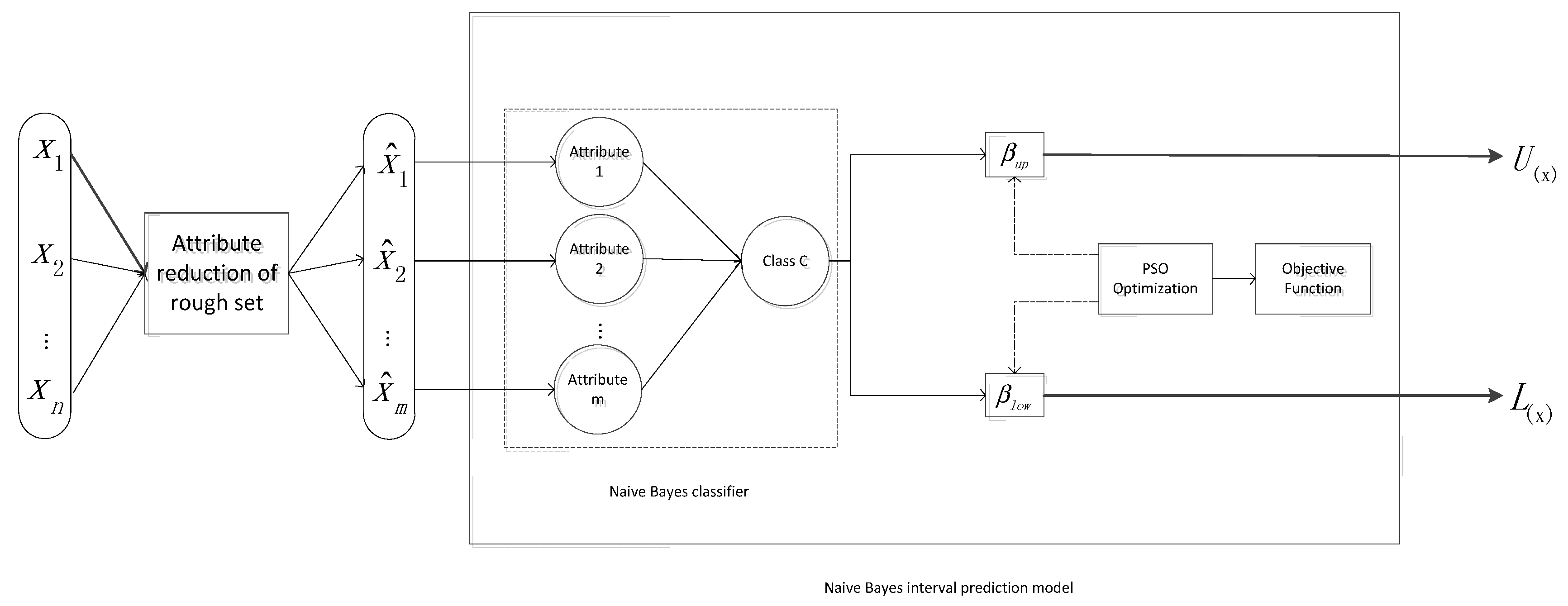
Figure 2.
Naive Bayesian classification model.

Figure 3.
Flow chart of attribute reduction in rough sets.

Figure 4.
Flowchart of proposed Naive Bayesian prediction intervals model.
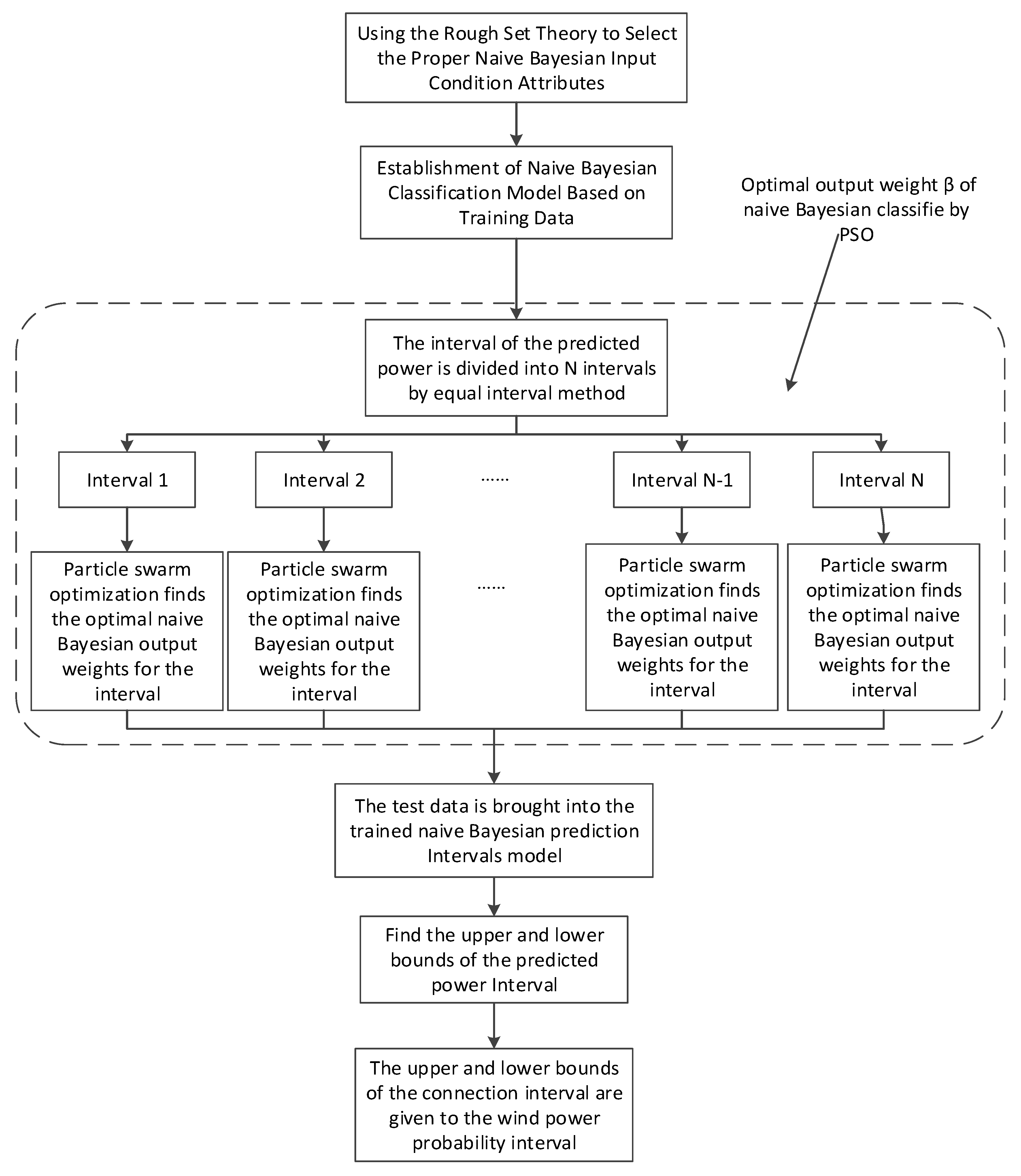
Figure 5.
Prediction intervals at 80% confidence level.

Figure 6.
Prediction intervals at 85% confidence level.

Figure 7.
Prediction intervals at 90% confidence level.

Figure 8.
The prediction intervals of segmented optimization and non-segmented optimization at an 85% confidence level: (a) segmented optimization and (b) non-segmented optimization.
Figure 8.
The prediction intervals of segmented optimization and non-segmented optimization at an 85% confidence level: (a) segmented optimization and (b) non-segmented optimization.

Table 1.
Decision table after discretization.
| Object | Condition Attribute | Decision Attribute | ||||||
|---|---|---|---|---|---|---|---|---|
| 1 | 5 | 3 | 5 | 7 | 3 | 10 | 5 | 3 |
| 2 | 6 | 5 | 6 | 3 | 8 | 18 | 9 | 6 |
| 3 | 4 | 5 | 4 | 9 | 6 | 7 | 5 | 4 |
| 11 | 10 | 14 | 19 | 6 | 7 | 10 | 14 | |
| 5 | 8 | 12 | 9 | 10 | 18 | 14 | 15 | 9 |
| 6 | 10 | 8 | 8 | 16 | 13 | 12 | 15 | 11 |
Table 2.
Significance degree of condition attribute.
| Wind Speed | Wind Speed | Wind Speed | Power | Power | Power | Power |
|---|---|---|---|---|---|---|
| 0.2778 | 0.1333 | 0.1222 | 0.1889 | 0.1667 | 0.0667 | 0.0444 |
Table 3.
Optimal output weights.
| 1 | 1.5922 | 0.4444 |
| 2 | 1.1994 | 0.7783 |
| 3 | 1.2241 | 0.8524 |
| 4 | 1.1370 | 0.8137 |
| 5 | 1.2439 | 0.9198 |
| 6 | 1.0971 | 0.8911 |
| 7 | 1.1475 | 0.9324 |
| 8 | 1.1355 | 0.9447 |
| 9 | 1.0187 | 0.8761 |
| 10 | 1.1016 | 0.8751 |
Table 4.
Prediction results using different methods.
| Confidence Level/% | Method | PICP/% | PINAW |
|---|---|---|---|
| 80 | NBC | 79.56 | 237.3430 |
| RS-NBC | 80.22 | 217.4590 | |
| RS-PSO-NBC | 80.87 | 190.2462 | |
| 85 | NBC | 84.84 | 269.3378 |
| RS-NBC | 85.27 | 272.8840 | |
| RS-PSO-NBC | 85.51 | 228.8553 | |
| 90 | NBC | 89.67 | 307.1498 |
| RS-NBC | 90.33 | 296.1640 | |
| RS-PSO-NBC | 90.45 | 271.6239 |
© 2017 by the authors. Licensee MDPI, Basel, Switzerland. This article is an open access article distributed under the terms and conditions of the Creative Commons Attribution (CC BY) license (http://creativecommons.org/licenses/by/4.0/).
Share and Cite
MDPI and ACS Style
Yang, X.; Fu, G.; Zhang, Y.; Kang, N.; Gao, F. A Naive Bayesian Wind Power Interval Prediction Approach Based on Rough Set Attribute Reduction and Weight Optimization. Energies 2017, 10, 1903. https://doi.org/10.3390/en10111903
AMA Style
Yang X, Fu G, Zhang Y, Kang N, Gao F. A Naive Bayesian Wind Power Interval Prediction Approach Based on Rough Set Attribute Reduction and Weight Optimization. Energies. 2017; 10(11):1903. https://doi.org/10.3390/en10111903
Chicago/Turabian StyleYang, Xiyun, Guo Fu, Yanfeng Zhang, Ning Kang, and Feng Gao. 2017. "A Naive Bayesian Wind Power Interval Prediction Approach Based on Rough Set Attribute Reduction and Weight Optimization" Energies 10, no. 11: 1903. https://doi.org/10.3390/en10111903
Note that from the first issue of 2016, this journal uses article numbers instead of page numbers. See further details here.