Indicative Fault Diagnosis of Wind Turbine Generator Bearings Using Tower Sound and Vibration †


Department of Mechanical and Manufacturing Engineering, University of Calgary, 2500 University Dr NW, Calgary, AB T2N 1N4, Canada
*
Author to whom correspondence should be addressed.
†
This paper is an extended version of our paper published in 24th International Congress on Sound and Vibration (ICSV 24), London, UK, 26 July 2017.
Energies 2017, 10(11), 1853; https://doi.org/10.3390/en10111853
Submission received: 7 September 2017
/
Revised: 27 September 2017
/
Accepted: 17 October 2017
/
Published: 13 November 2017
(This article belongs to the Special Issue Wind Turbine Loads and Wind Plant Performance)
Abstract
:The idea of indicative fault diagnosis based on measuring the wind turbine tower sound and vibration is presented. It had been reported by a wind farm operator that a major fault on the generator bearing causes shock and noise to be heard from the bottom of the wind turbine tower. The work in this paper was conceived to test whether tower top faults could be identified by taking simple measurements at the tower base. Two accelerometers were attached inside the wind turbine tower, and vibration data was collected while the wind turbine was in operation. Tower vibration signals were analyzed using Empirical Mode Decomposition and the outcomes were correlated with the vibration signals acquired directly from the generator bearings. It is shown that the generator bearing fault signatures were present in the vibrations from the tower. The results suggest that useful condition monitoring of nacelle components can be done even when there is no condition monitoring system installed on the generator bearings, as is often the case for older wind turbines. In the second part of the paper, acoustic measurements from a healthy and a faulty wind turbine are shown. The preliminary analysis suggests that the generator bearing fault increases the overall sound pressure level at the bottom of the tower, and is not buried in the background noise.
1. Introduction
According to a wind farm operator, shock and sound of vibration can be heard from the base of the wind turbine, when there is a major generator bearing fault. This motivated the authors to think of a way to supplement these perceptions with simple measurements. The purpose of this paper is to study whether vibration and acoustic signals taken at the bottom of the wind turbine tower can yield useful information in support of the reporting of the wind farm technicians. This is important since this type of analysis could allow wind turbine operators to identify if there is any fault in the generator bearings from simple measurements at ground level, before performing more complicated vibration analysis.
To the authors’ knowledge, there have been no similar studies reported in the literature, thus the analysis in this article may open a new window for extension and more research.
The rest of the paper describes the main findings of this study and is organized as follows. Section 2 provides a brief overview of the operation and maintenance approaches for wind turbine drive-trains. In Section 3, signal modulation and bearing characteristic frequencies for variable speed condition, Empirical Mode Decomposition as the vibration analysis tool used in this paper, and fundamentals of acoustic analysis are described. Section 4 presents vibration analysis conducted on the data collected directly from the generator bearing. Section 5 and Section 6 discuss the important results derived from the vibration and acoustic analyses of the wind turbine tower, respectively. Section 7 summarizes the key conclusions drawn from this feasibility study.
2. Wind Turbine Drive-Train Operation Monitoring
Unlike conventional power plants, it is expensive to physically visit wind turbines for operation monitoring and maintenance, due to their location, tower height, and environmental conditions [1]. As a result, condition monitoring has represented a growing area and opportunity in the wind power industry. Generally, there are three main strategies utilized by the industry: reactive, preventive and predictive maintenance [2]. Reactive strategy [3] means to run a component in the nacelle until it is damaged and cannot operate any further. Then, the repair is performed, which is typically a part replacement, and operation resumes until the next incident. This strategy is not cost effective because sudden component repairs and replacement could cost much more than planned maintenance. In addition, the breakdown of a component in the drive-train would damage other components, which itself is an additional cost. For instance, the total revenue loss (direct and indirect) due to a generator bearing failure can reach $20,000–$30,000 a wind turbine, according to a large wind farm operator in Canada.
Preventive maintenance [4] is a planned maintenance strategy that is triggered and scheduled based on events. It is also called time-based maintenance. It relies greatly on operator experience, age of the machine, and also manufacturer recommendations. The main assumption is that an operating component has a certain service life expectancy and is to be replaced or repaired at specific time frames. However, the intervals between services are usually too long to detect a defect at its early stage. In addition, the same type of components in different turbines develop faults at different times and rates.
Predictive maintenance [5] is the cost-optimal strategy. It is performed by monitoring the status of the machine, based on different sets of data (i.e., vibration, oil, temperature, etc.). It is also called condition-based maintenance. The operator can detect faults as early as possible by analyzing the data, and schedule proper maintenance. For example, wind turbine operators in Canada tend not to schedule any maintenance in winter time because of the harsh weather and the associated cost. If they follow the reactive or preventive maintenance strategies, a sudden breakdown of a component might occur in winter and they must then shut down the wind turbine and replace the part. However, if the defect is detected early enough by data analysis, temporary remedies can delay the breakdown, and the part can be replaced in the spring or summer. Through this strategy, wind turbine operators can also repair or replace a group of parts at the same time, as one of the substantial costs of wind turbine repair is the cost of crane rental [6]. Instead of renting a crane for a few days to change only one part, they can replace a group of damaged components on several wind turbines in the farm.
A study of over a thousand wind turbines with faulty generators showed that bearing failure is the dominant cause of generator failure, responsible for about 60% of failures [7]. Bearing damage is most commonly due to excessive load, overheating, fatigue, brinelling, improper lubrication, contamination, corrosion, and shaft misalignment [8]. Fault diagnosis is the first step of the predictive maintenance approach, which is performed before root causes analysis and prognosis. There are three main techniques to diagnose bearing faults within the wind energy industry; oil analysis, temperature analysis, and vibration analysis. Vibration analysis is perhaps the most efficient type of bearing defect detection method [9]. An undamaged bearing generates a stationary vibration theoretically; however, faults on the bearing elements introduce impulses at specific frequencies depending on the location of them, and consequently amplify the vibration at a specific frequency band. Vibration analysis techniques including time domain, frequency domain and combination of time and frequency domains have been used for a long time and have significantly improved over the last two decades. Today’s installed large wind turbines are typically equipped with vibration sensors on different components of the drive-train such as main bearing, gearbox, gearbox bearings, and generator bearings. An operation centre monitors the status of the drive-train remotely [10]. For a typical 1.5 MW wind turbine, eight to eleven vibration sensors are installed [11]. For the turbine studied in this paper, there is one sensor on the main bearing, six on the gearcase, and four on the generator bearings (two on drive-end and two on non-drive-end bearings). A modern wind company may own hundreds or thousands of turbines, most likely a range of models from multiple manufactures, which makes handling the large amount of monitoring data difficult and time consuming if each turbine has a large number of sensors. For example, a typical 200 MW wind farm in Canada includes 133 wind turbines (each 1.5 MW). With eleven vibration sensors on each wind turbine drive-train and a common sampling interval of 10 min, one could realize the required effort to monitor the operations. This excludes other types of sensors, such as oil and temperature sensors, which increase the volume of data mining. In this case, there may be considerable benefit from the simple monitoring described in this paper, which could indicate the turbines to concentrate on for detailed study. Moreover, many old wind turbines do not have online vibration monitoring; thus, the described method would bring advantage to the monitoring scheme of such turbines.
3. Basic Theory
3.1. Bearing Fault Characteristics and Modulation
Bearings could generate five defect frequencies: outer race pass, inner race pass, cage or fundamental train, rolling element spin, and twice rolling element spin, as described below. The combination of the gearbox mesh frequencies, bearing defect frequencies, harmonics, and other noise sources in the derive-train can generate a complex signal. Additionally, the shaft speed varies with the wind speed, and therefore characteristic frequencies of the bearing and gearbox also change with speed.
When a rolling element passes over a defect for example on the inner or outer races, the temporary loss of contact causes a deflection of the element. When the element hits the far side of the defect, regaining the contact generates an impact on the bearing structure [12]. It is believed that the impacts excite the bearing structure’s natural frequencies. This excitation happens each time a rolling element hits the defect, so an impulse response is produced. Therefore, a series of impulses repeating at the relevant fault frequency is produced. This leads to a series of amplitude modulated impulses in the vibration signal, where the content appears as changes in the amplitude of the so-called carrier signal of the bearing (i.e., natural frequency). The carrier frequency is typically in the range of 2 to 10 kHz for wind turbine generator bearings [13].
The impulse frequency is called the characteristic frequency. Depending on the location of the fault, these frequencies are [14]:
- Ball passing outer race frequency:
- Ball passing inner race frequency:
- Fundamental train frequency (Cage speed):
- Ball spin frequency:
In the above equations, d, D, , , and n are the diameter of the rolling elements, pitch diameter, shaft rotational frequency, contact angle between the rolling elements and the raceway, and number of rolling elements, respectively, as shown in Figure 1.
Amplitude modulation of a signal results in pairs of sidebands in the spectrum, spaced around the bearing carrier frequency equal to the modulation frequency. Therefore, vibration enveloping (also called amplitude demodulation [15]) demodulates signals and separates the fault frequency from the carrier frequency. When properly configured, vibration enveloping will usually have a much higher sensitivity to faults that produce impacting.
3.2. Vibration Analysis Using Empirical Mode Decomposition
Empirical Mode Decomposition (EMD) is an adaptive decomposition technique used for non-stationary and nonlinear signals [16], without changing the time domain. The overall idea is similar to other decomposing techniques such as short-time Fourier transform or Wavelet decomposition. It starts decomposing a signal from a local oscillation level. The decomposed modes unlike other decomposition methods such as Discrete Wavelet Transform are not necessarily orthogonal, and they are sufficient to reconstruct the original signal, since there is no external windowing function. The key step in EMD is to identify the oscillatory modes defined by the interval between local extrema. The decomposed modes are called Intrinsic Mode Functions (IMF) that meet the following conditions:
- Each IMF has only one extremum between zero crossings,
- Each IMF has a mean value of zero.
An IMF represents a simple oscillatory mode and could contain a variable amplitude and frequency as functions of time [17]. Therefore, in order to start decomposing, one can identify all local extrema of the signal, , to create the upper and lower envelopes [18]. The mean envelope is called m. It is shown in Figure 2 where the blue line is the original signal, the red line is the upper envelope, the green is the lower envelope, and the black line is the mean envelope. The overall procedure can be written as:
where and are the original signal (), and its the mean envelope, respectively. If does not meet the above two conditions, the iteration process continues (i.e., j increases). This procedure is called sifting, and continues until meets the conditions to be called an IMF. The subsequent modes, IMFi, are produced by repetition of the same algorithm. The signal then can be represented as:
where n is the number of modes and is the residue.
There are a few drawbacks with EMD. The major one is the appearance of mode mixing, which is different modes of oscillations coexisting in a single IMF due to signal intermittency [17]. As such, Huang et al. [17] proposed a noise-assisted scheme, known as Ensemble EMD (EEMD), “which defines the true IMF components as the mean of an ensemble of trials, each consisting of the signal plus a white noise of finite amplitude” [19]. In other words, based on the ensemble number (N), white noises with the same amplitude are added N times to the original signal to generate N modified signals. Then, EMD is applied on each modified signal to create sets of IMFi. Consequently, each final IMF is calculated by averaging the N IMF included in one set. White noises in a time space ensemble mean cancel each other out, and only the signal in the final noise-added signal ensemble mean comes out. The additional white noise populates the time-frequency space uniformly. Details can be found in the literature, such as [20].
It is worth mentioning that a signal collected from the wind turbine tower contains, but is not limited to, the gearbox mesh frequencies, harmonics, bearing characteristic frequencies, and other mechanical noise sources in the nacelle, all transmitted through the tower. The tower is a long pathway that potentially attenuates the signal. In addition, as the tower is anchored to the ground, it is also subjected to ground vibration contamination. EMD/EEMD can help with decomposing the collected signal, and extracting a part of the signal that is applicable for the subsequent vibration analysis.
3.3. Sound Level Fundamentals
In this section, sound level fundamentals are presented, which are used for further analysis later. Sound is generated by pressure fluctuations in the air with regard to the static air pressure. In other words, it is the difference between the pressure generated by a sound wave and the ambient pressure at the same point in space. Commonly, the atmospheric pressure is defined as Pa [21]. The fluctuation can be below or above the atmospheric pressure. To quantify the sound pressure, the root mean square (RMS) of the square of the fluctuations is calculated. Because of the wide range of human hearing, the use of absolute sound pressure values are impracticable. Thus, the logarithmic scale (dB) with respect to the threshold of hearing is typically used. The threshold of hearing is Pa.
4. Fault Diagnosis of Generator Bearing
The fault diagnosis of a generator bearing of an operating wind turbine in a 70 MW wind farm located in Canada is described in this section.
The vibration data was recorded with accelerometers with sensitivity of 100 mV/g, sampled at 25.6 kHz from the online vibration monitoring system on the 1.5 MW wind turbine with 80 m tower. Bearing parameters are: d = 4.5 cm, D = 23.5 cm, = 0, and n = 9. Based on bearing’s geometry, the characteristic defect frequencies of the bearing are: BPFO = 3.64 , BPFI = 5.36 , FTF = 0.4 , and BSF = 2.5 . Figure 3 shows one set of the vibration data, taken in September, 2015, and the spectrum arbitrarily chosen from the data set. There is a cluster of high amplitude components and sidebands around 6000 Hz. The data was denoised using the algorithm proposed by the author in [22]. Briefly, the original signal () was decomposed using EEMD to calculate IMFs. Then, the following parameter (I) was calculated for each IMF:
where is the Kurtosis factor calculated for each decomposed mode, and RMS () is the root mean square function. This parameter is intended to reflect a combination of peakiness and energy of the decomposed modes. It was shown in [22] that using only Kurtosis factor for mode selection and denoising might lead to incorrect results, since Kurtosis factor does not take energy of the signal into account. Then, the IMF which has the highest I value is identified, called the Ith IMF. A new signal is reconstructed as:
where n is the number of decomposed modes. This reconstructed signal, then, does not include the modes in higher frequency bands than Ith IMF. EEMD is applied again on the reconstructed signal, and the IMF that has the highest I value is identified. These iterations are repeated until . The final denoised signal, , after iterations is:
Figure 4 shows the order tracked results after EEMD was applied. White noise with a standard deviation of 0.1 and the ensemble size of 100 were used. The order of 3.6 and its harmonics are excited, that is the outer raceway fault order. The integer orders refer to the shaft speed orders.
5. Wind Turbine Tower Vibration Analysis
As mentioned, it has been reported that sound of vibration and shock can be heard from the bottom of the wind turbine in the case of major fault on the generator bearing. The purpose of this section is to identify whether vibration signals taken from the bottom of the turbine structure show the same faults as picked up from the data collected by the accelerometers attached to the generator bearing housing. This method could be considered as a combination of both preventive and predictive monitoring approaches. The tower vibration measurement/analysis is essentially a time-based monitoring, yet, depending on the results from the analysis, the next step, which is a detailed vibration analysis on the data collected from the generator bearing, is a predictive monitoring.
RMS value is typically the first indicator used by the wind turbine operators to identify the state change of running components. It started to increase significantly over a period of seven months for this particular wind turbine as shown in Figure 5.
The red curve highlights the increasing trend. The increasing RMS trend was not a transient incident similar to what happened soon after June 2013. Therefore, there was a bearing fault. Other rotating components such as main bearing, gearbox, gearbox bearings had their vibration RMS level at a “normal” level, thus the chance of generating defect frequencies were low, again according to the operator’s diagnosis centre.
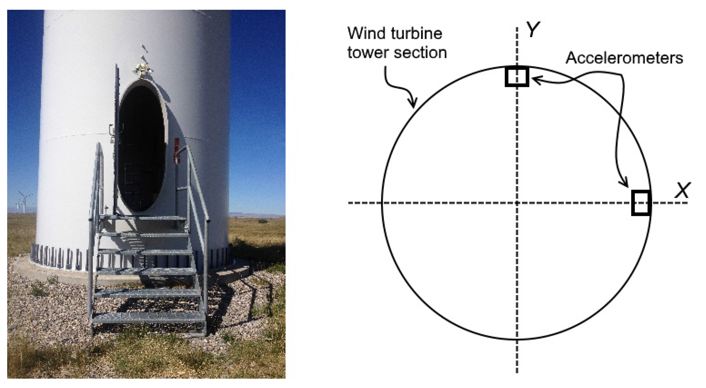
The vibration data for this section were collected at the bottom of the tower by two piezoelectric accelerometers attached orthogonally inside of the tower (see the picture and schematic showing the locations of the accelerometers in Figure 6), with sampling frequency of 25.6 kHz and sensitivity of 100 mV/g. Since bearing fault frequencies tend to be carried by a carrier signal and the vibration could vary between along-wind and across-wind, the idea was to use two accelerometers; thus, tower structural frequencies in the arbitrary x and y directions were acquired while the wind turbine was yawing, and the chance of collecting bearing vibration transmitted through the tower was increased. After the experiment, it was revealed that the vibration signals from both directions were similar with the same order of amplitude. For the analysis conducted in the next sections, vibration signals from both directions were used.
5.1. Parked Condition
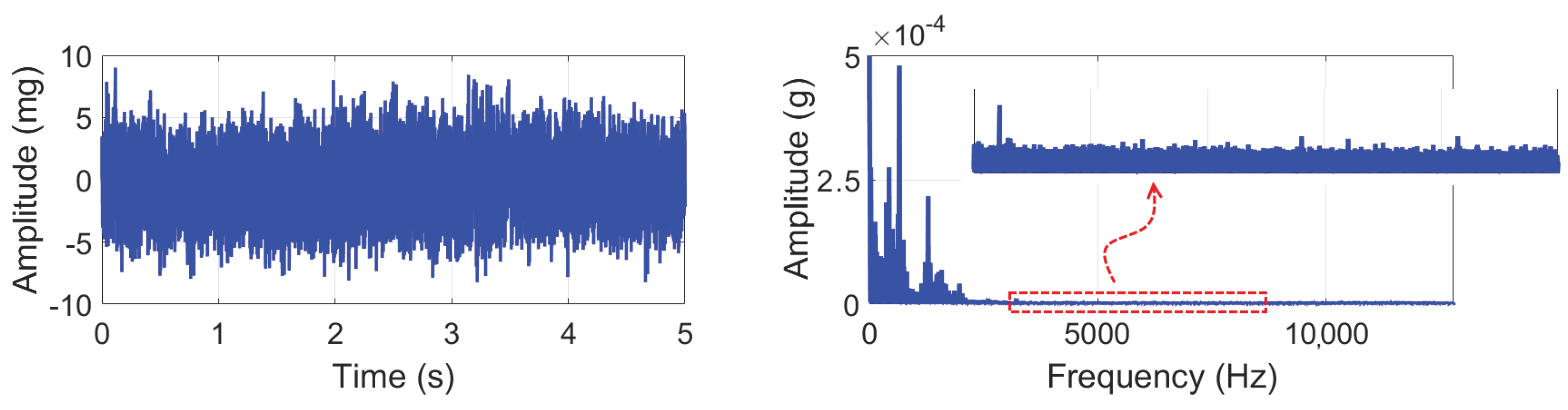
Here, collected vibration data while the wind turbine was in the parked condition are analyzed. Both drive-train and electrical equipment inside of the tower were shutdown. Wind was the only excitation to the whole structure. The average wind speed during this test was 8.6 m/s, which was well above the cut-in wind speed, 3.5 m/s. Figure 7 shows a section of vibration data and its spectrum. Frequencies above ~2000 Hz indicate no significant peaks, as shown by the zoomed-in section. This was expected, as only structural frequencies that are typically in a lower frequency bands were excited due to the wind.
5.2. Operating Conditions
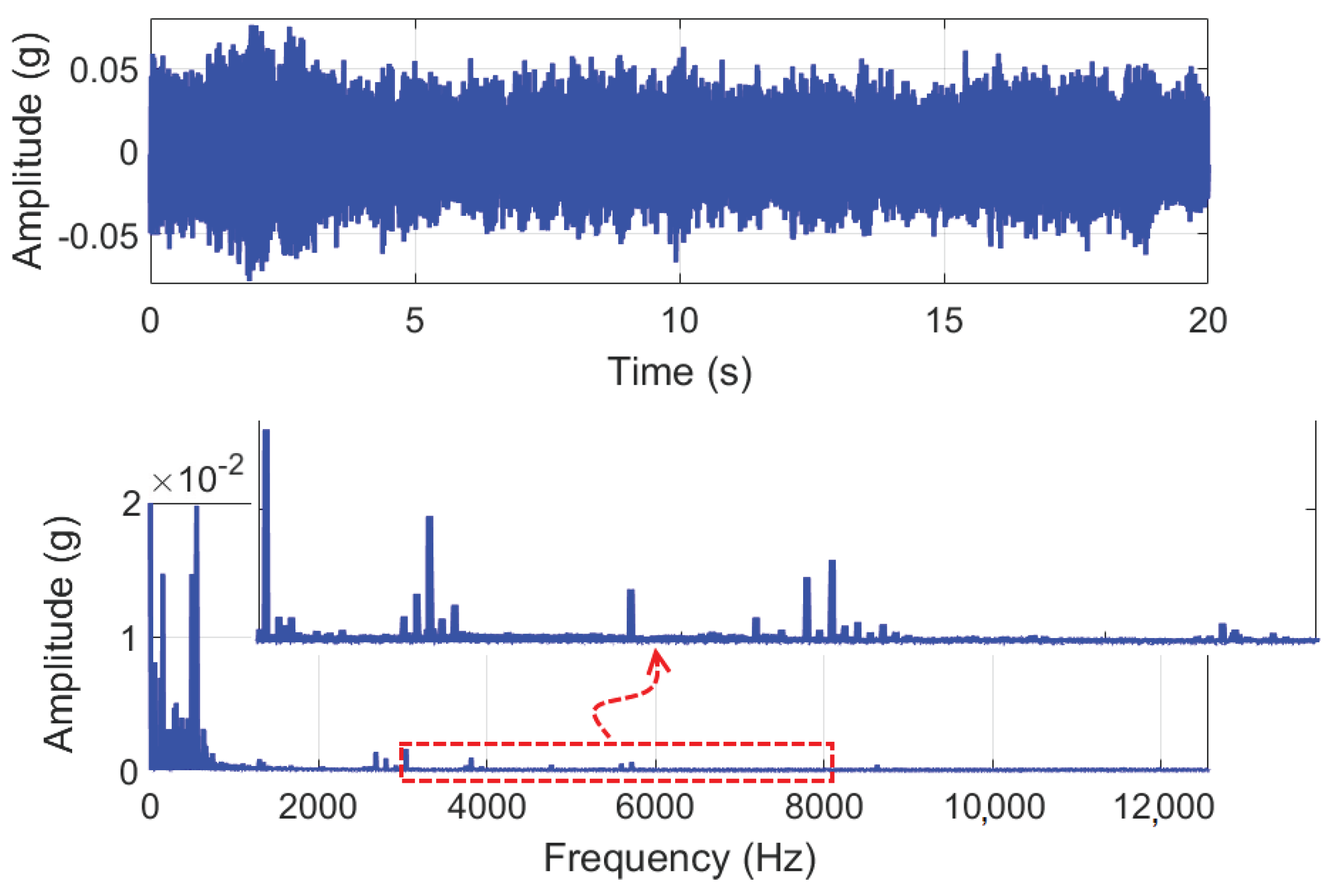
The main test was carried out while the turbine was operating. Figure 8 shows a sample of the tower vibration signal, after DC offset component was removed. The vibration level was between ±0.1 g, which was 10 times higher than the parked condition. In the spectrum, the majority of high peaks are located in the lower frequency range, corresponding to the tower’s structural frequencies, as seen in the parked and also in the operating conditions. The order of amplitude is about 40 times higher than the parked condition, which was expected.
It may not be very visible from the figure; however, there are small peaks spaced at exactly 60 Hz, which is the generated electricity frequency.
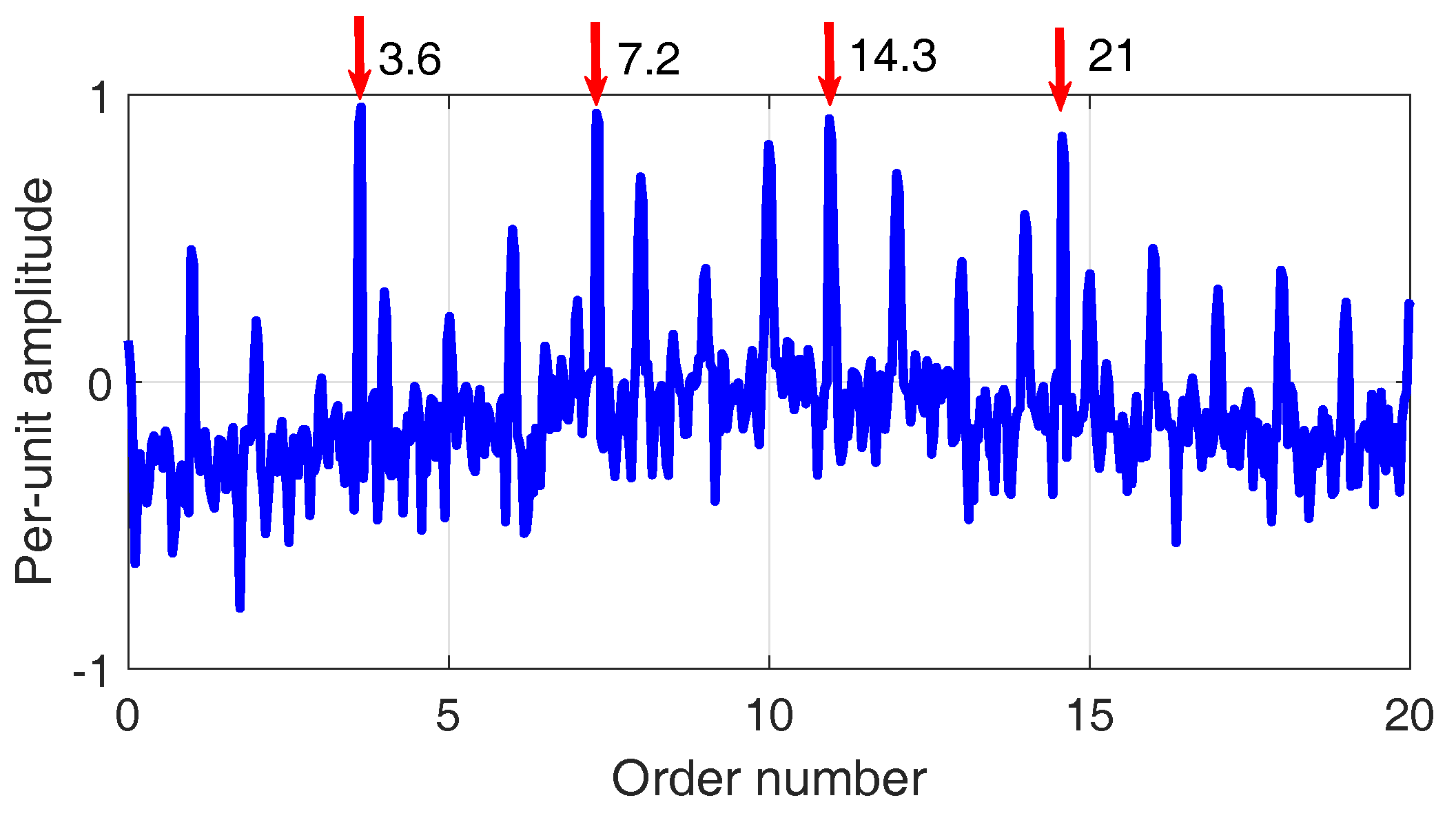
EEMD was used to decompose the signal into IMFs, as shown in Figure 9 with normalized spectra. Spectra suggest that excited frequencies except IMF2 and IMF3 are in lower frequency bands, which relate to tower characteristic frequencies and low frequency excitation from the wind and drive-train components. Time-domain IMFs were correlated with the vibration data collected from the generator bearing housing. The highest value is linked to IMF2, which means that the second decomposed mode is more similar to the bearing vibration.
The order diagram in Figure 9 is linked to the second IMF, where the order of 3.6 and the next two harmonics are excited. They are highlighted by red arrows. Although the magnitude is very low, in the range of , it is an indication of the BPFO on the generator bearing, which is consistent with the results derived in Section 4.
6. Wind Turbine Tower Acoustic Tests
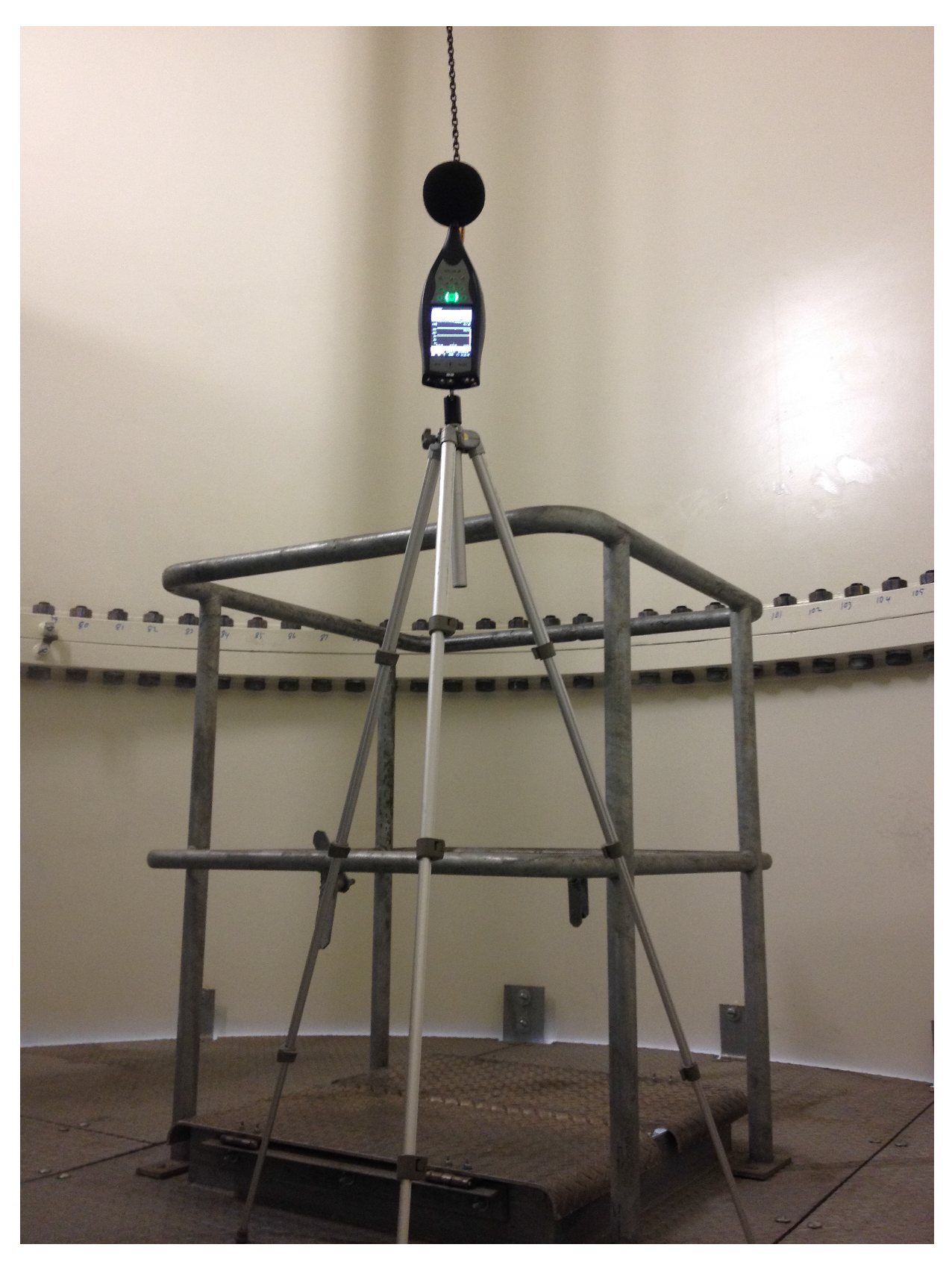
In this section, the main findings and results from several acoustic measurements are presented. In order to measure the sound propagated inside of the tower, a Sound Pressure Level (SPL) meter was used, as shown in Figure 10.
The SPL was a B & K 2250 sound analyzer (Brüel & Kjær, Nærum, Denmark), capable of measuring 0.5 Hz to 20 kHz broadband range. The equipment was placed at the centre of the tower, one level above the transformer.
Several measurements from two wind turbines were conducted, next to each other. “Turbine 1” was the turbine with a healthy drive-train, and “Turbine 2” with the faulty bearing. Wind speed at the time of each measurement was also available from the production database. Table 1 lists the main measurements. SPL meter was set up to record ambient (LA) continuously for different condition of wind turbine operations.
The background noise can be determined when the wind turbine and all equipment are switched off, which is the first case for both turbines. As Turbine 1 starts to operate, with the transformer being switched off, the sound level increases to 66.82 dBA. These measurements were recorded with different wind speeds. However, the effect of wind speed on the recorded sound level inside of the tower is small. Comparing cases 3, 4, and 5 from Turbine 1 (where wind speed more than doubled) suggests that the fully operating wind turbine generates 81–82 dBA inside of the tower. Similar conclusions can be drawn by comparing cases 2, 3, and 4 from Turbine 2.
Based on the observations during the acoustic measurements, the following equation can be written, which includes the major components of the measured total sound level, :
where , , , and are background, transformer, drive-train, and other sources of the noise, respectively. Since the wind speed seemed to have an insignificant effect on the total SPL inside of the tower, each component can be estimated by averaging different measurements:
- = 61.38 dBA (average of Case 1 for Turbines 1 and 2),
- = 79.42 dBA (Case 3 − Case 2 for Turbine 1),
- = 82.25 dBA (average of Cases 2, 3 and 4 for Turbine 2).
- : This source of noise could be, for example, moving cables, and any other type of extra noises. During the measurements, the environment was controlled so that extra noise was minimized. Here, it is assumed 0 dBA.
Therefore, = 67.71 dBA, which is an estimation of the sound level emitted by the faulty generator bearing.
It should be noted that the acoustic measurements were rough, and only a feasibility study was the purpose of this analysis. However, it appears that a fault in the drive-train generates a considerable amount of sound/noise, and it is not buried in the background noise. Sound spectrum, which is recorded by a more advanced SPL meter, could show which frequency band is excited by the fault.
7. Conclusions
We have demonstrated indicative fault diagnosis of wind turbine generator bearings from vibration measurements on the wind turbine tower. Two accelerometers were attached orthogonally inside of the tower to collect tower vibration. Vibration analysis using EEMD and correlation factor suggest evidence of the bearing fault frequency/order on the tower vibration. Vibration analysis on the data collected directly from the generator bearing housing suggested the same result. This idea can be investigated more for potential establishment of an indicative fault detection scheme, which essentially may reduce the amount of effort required for wind farm operation data mining, and indicate the wind turbines to concentrate on for detailed analysis. The RMS of the studied wind turbine in this paper was considerably high, and a similar analysis is to be applied accordingly on turbines with less severe faults. This may demand more advanced signal processing tools with higher sensitivity and resolution.
In the second part of the paper, acoustic measurements using a SPL meter was shown. Preliminary analysis on the overall sound level indicated that the generated sound/noise due to the generator bearing fault is not buried in the background noise, and is distinguishable. A detailed study on the sound spectrum could reveal which frequency band is excited because of it.
Acknowledgments
This research was supported by the Natural Science and Engineering Research Council of Canada (NSERC) under the Industrial Research Chair program, ENMAX Corp. (Calgary, AB, Canada), and the Research and Development Engage program. We thank TransAlta Corp. (Calgary, AB, Canada) for providing the bearing vibration data and allowing us access to their wind farm to collect the tower vibration and acoustic data.
Author Contributions
Ehsan Mollasalehi conducted the vibration and acoustic measurements, and analyses were supervised by David Wood and Qiao Sun.
Conflicts of Interest
The authors declare no conflict of interest.
Abbreviations
The following abbreviations are used in this manuscript:
| BPFO | Ballpass frequency, outer race |
| BPFI | Ballpass frequency, inner race |
| FTF | Fundamental train frequency (Cage) |
| BSF | Ball spin frequency |
| FFT | Fast Fourier transform |
| EMD | Empirical mode decomposition |
| EEMD | Ensemble empirical mode decomposition |
| IMF | Intrinsic mode function |
| RMS | Root mean square |
| SPL | Sound pressure level |
References
References
- Tchakoua, P.; Wamkeue, R.; Ouhrouche, M.; Slaoui-Hasnaoui, F.; Tameghe, T.A.; Ekemb, G. Wind turbine condition monitoring: State-of-the-art review, new trends, and future challenges. Energies 2014, 7, 2595–2630. [Google Scholar]
- Walford, C.A. Wind Turbine Reliability: Understanding and Minimizing Wind Turbine Operation and Maintenance Costs; Department of Energy: Washington, DC, USA, 2006.
- Swanson, L. Linking maintenance strategies to performance. Int. J. Prod. Econ. 2001, 70, 237–244. [Google Scholar] [CrossRef]
- Nilsson, J.; Bertling, L. Maintenance management of wind power systems using condition monitoring systems—Life cycle cost analysis for two case studies. IEEE Trans. Energy Convers. 2007, 22, 223–229. [Google Scholar] [CrossRef]
- Kusiak, A.; Li, W. The prediction and diagnosis of wind turbine faults. Renew. Energy 2011, 36, 16–23. [Google Scholar] [CrossRef]
- Martin-Tretton, M.; Reha, M.; Drunsic, M.; Keim, M. Data Collection for Current US Wind Energy Projects: Component Costs, Financing, Operations, and Maintenance; National Renewable Energy Laboratory: Golden, CO, USA, 2012; Volume 303, pp. 275–3000.
- Alewine, K.; Chen, W. A review of electrical winding failures in wind turbine generators. In Proceedings of the 2011 Electrical Insulation Conference (EIC), Annapolis, MD, USA, 5–8 June 2011; pp. 392–397. [Google Scholar]
- Radu, C. The Most Common Causes of Bearing Failure and the Importance of Bearing Lubrication. RKB Technical Review. 2010. Available online: http://www.rkbbearings.com/en/publications.php (accessed on 10 November 2017).
- Wang, W.; Jianu, O.A. A smart sensing unit for vibration measurement and monitoring. IEEE/ASME Trans. Mechatron. 2010, 15, 70–78. [Google Scholar] [CrossRef]
- Hyers, R.; McGowan, J.; Sullivan, K.; Manwell, J.; Syrett, B. Condition monitoring and prognosis of utility scale wind turbines. Energy Mater. 2013, 187–203. [Google Scholar] [CrossRef]
- Sheng, S.; Link, H.; LaCava, W.; Van Dam, J.; McNiff, B.; Veers, P.; Keller, J.; Butterfield, S.; Oyague, F. Wind Turbine Drivetrain Condition Monitoring during GRC Phase 1 and Phase 2 Testing.; National Renewable Energy Laboratory: Golden, CO, USA, 2011.
- Ho, D.; Randall, R. Optimisation of bearing diagnostic techniques using simulated and actual bearing fault signals. Mech. Syst. Signal Process. 2000, 14, 763–788. [Google Scholar] [CrossRef]
- Mollasalehi, E.; Wood, D.; Sun, Q. Bearing fault diagnosis using empirical mode decomposition based order tracking, wind turbine generator application. In Proceedings of the 23rd International Congress on Sound and Vibration 2016 (ICSV 23): From Ancient to Modern Acoustics, Athens, Greece, 10–14 July 2016; pp. 4466–4473. [Google Scholar]
- McFadden, P.; Smith, J. Vibration monitoring of rolling element bearings by the high-frequency resonance technique—A review. Tribol. Int. 1984, 17, 3–10. [Google Scholar] [CrossRef]
- Mollasalehi, E.; Sun, Q.; Wood, D. Wind Turbine Generator Bearing Fault Diagnosis Using Amplitude and Phase Demodulation Techniques for Small Speed Variations. Adv. Cond. Monit. Mach. Non-Stn. Oper. 2016, 4, 385–397. [Google Scholar]
- Huang, N.E.; Shen, Z.; Long, S.R.; Wu, M.C.; Shih, H.H.; Zheng, Q.; Yen, N.C.; Tung, C.C.; Liu, H.H. The empirical mode decomposition and the Hilbert spectrum for nonlinear and non-stationary time series analysis. Proc. R. Soc. Lond. A Math. Phys. Eng. Sci. 1998, 454, 903–995. [Google Scholar] [CrossRef]
- Wu, Z.; Huang, N.E. Ensemble empirical mode decomposition: A noise-assisted data analysis method. Adv. Adapt. Data Anal. 2009, 1, 1–41. [Google Scholar] [CrossRef]
- Nunes, J.C.; Deléchelle, E. Empirical mode decomposition: Applications on signal and image processing. Adv. Adapt. Data Anal. 2009, 1, 125–175. [Google Scholar] [CrossRef]
- Shen, Z.; Wang, Q.; Shen, Y.; Jin, J.; Lin, Y. Accent extraction of emotional speech based on modified ensemble empirical mode decomposition. In Proceedings of the 2010 IEEE Instrumentation and Measurement Technology Conference (I2MTC), Austin, TX, USA, 3–6 May 2010; pp. 600–604. [Google Scholar]
- Žvokelj, M.; Zupan, S.; Prebil, I. EEMD-based multiscale ICA method for slewing bearing fault detection and diagnosis. J. Sound Vib. 2016, 370, 394–423. [Google Scholar] [CrossRef]
- Kinsler, L.E.; Frey, A.R.; Coppens, A.B.; Sanders, J.V. Fundamentals of acoustics. In Fundamentals of Acoustics, 4th ed.; Lawrence, E., Kinsler, A.R., Eds.; Wiley-VCH: Weinheim, Germany, 1999; Volume 1999, p. 560. ISBN 0-471-84789-5. [Google Scholar]
- Mollasalehi, E. Data-Driven and Model-Based Bearing Fault Analysis, Wind Turbine Application. Ph.D. Thesis, University of Calgary, Calgary, AB, Canada, 2017. [Google Scholar]
Figure 1.
Geometric parameters of a bearing-side view.
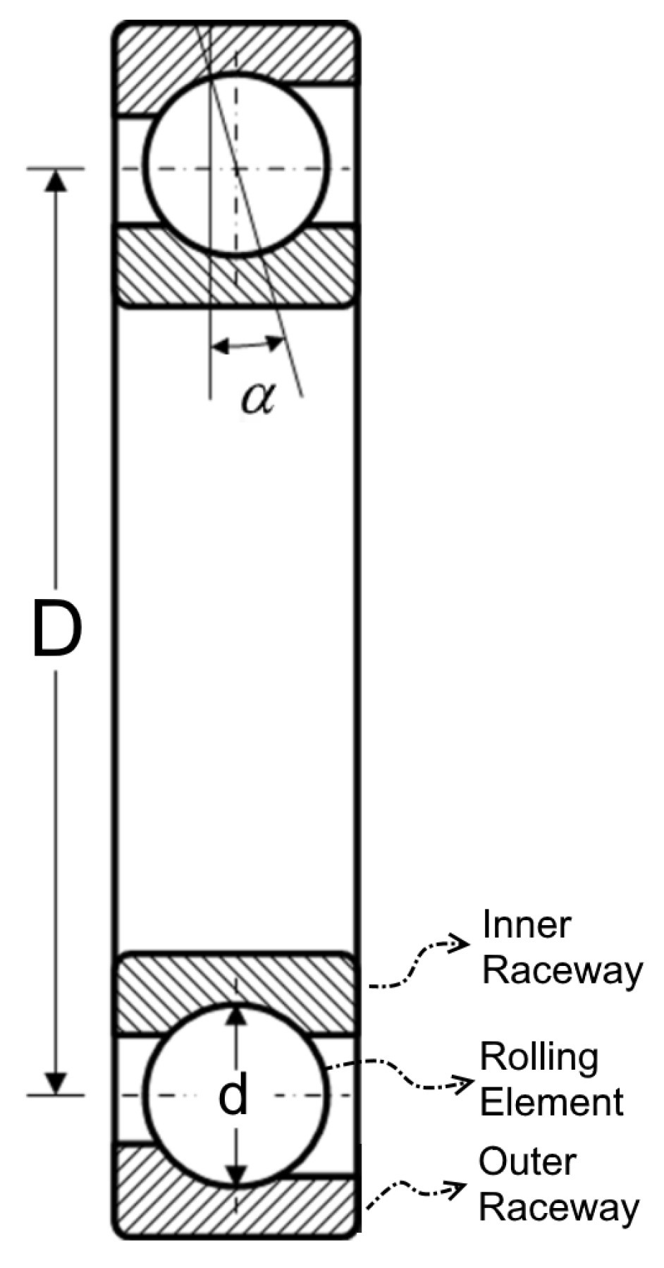
Figure 2.
Empirical mode decomposition sifting process—blue line is the signal, red line is the upper envelope, green is lower envelope, and black line is the mean envelope—Y axis represents any arbitrary amplitude.
Figure 2.
Empirical mode decomposition sifting process—blue line is the signal, red line is the upper envelope, green is lower envelope, and black line is the mean envelope—Y axis represents any arbitrary amplitude.
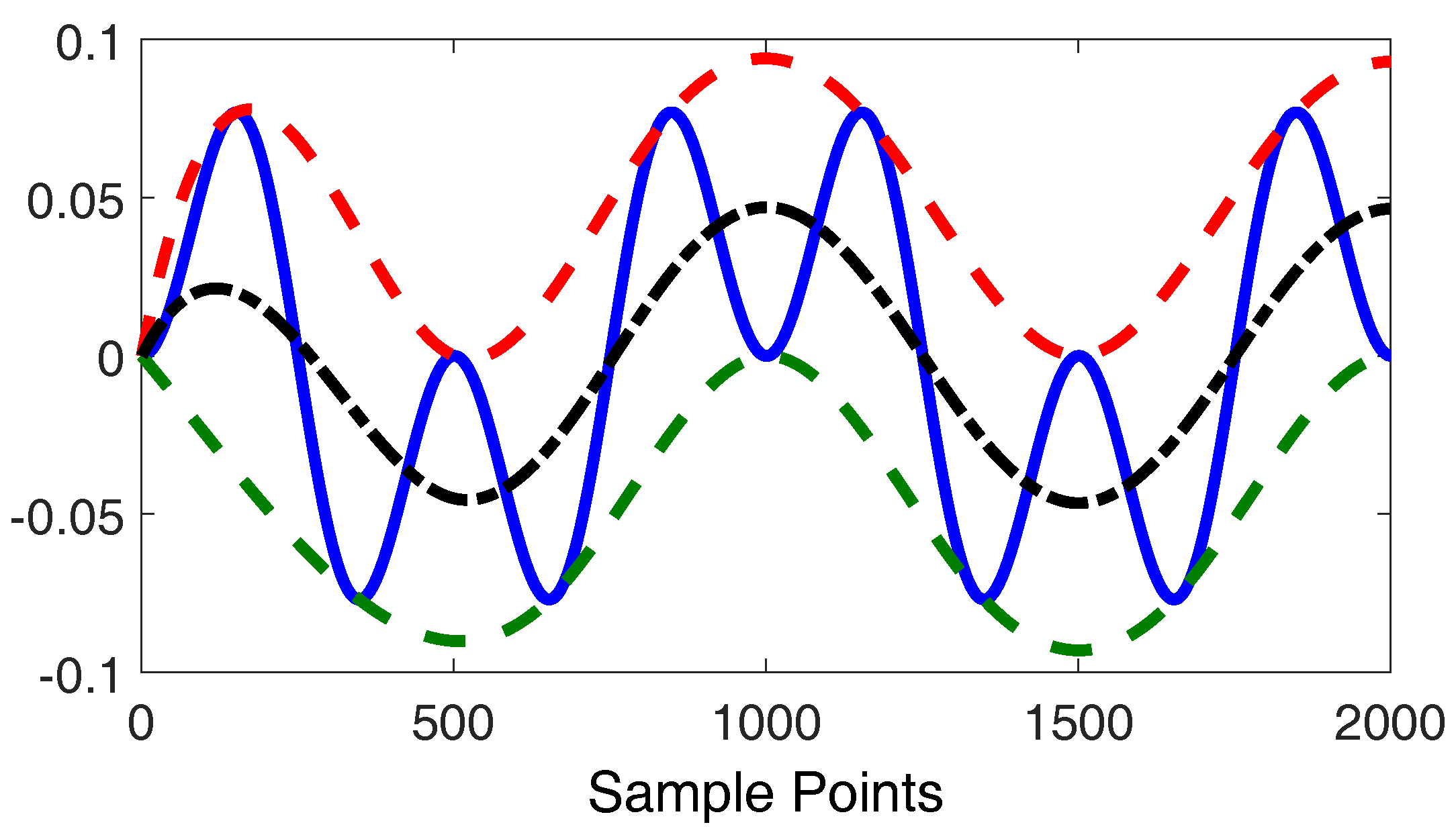
Figure 3.
(top) Vibration signal acquired from the generator bearing, (bottom) spectrum.

Figure 4.
Order analysis of the generator bearing signal suggesting outer race fault frequency order excitation (red arrows).
Figure 4.
Order analysis of the generator bearing signal suggesting outer race fault frequency order excitation (red arrows).

Figure 5.
Root mean square level development with time—the red curve shows the trend.

Figure 6.
(left) 1.5 MW wind turbine tower; (right) schematic of the location of the accelerometers on the wind turbine tower.
Figure 6.
(left) 1.5 MW wind turbine tower; (right) schematic of the location of the accelerometers on the wind turbine tower.

Figure 7.
A section of tower vibration in parked condition: (left) time domain; (right) frequency domain—zoomed-in area is highlighted in red.
Figure 7.
A section of tower vibration in parked condition: (left) time domain; (right) frequency domain—zoomed-in area is highlighted in red.

Figure 8.
Sample of the vibration data from the tower in the operating condition: (top) time domain; (bottom) frequency domain- zoomed area is highlighted by red.
Figure 8.
Sample of the vibration data from the tower in the operating condition: (top) time domain; (bottom) frequency domain- zoomed area is highlighted by red.

Figure 9.
(top left section) first 10 Intrinsic mode functions of the tower vibration; (top right) first six spectra of IMFs accordingly; (bottom left) first 10 correlation coefficients with generator bearing vibration; (bottom right) ordergram of the second IMF—red arrows refer to the outer race fault order and its harmonics.
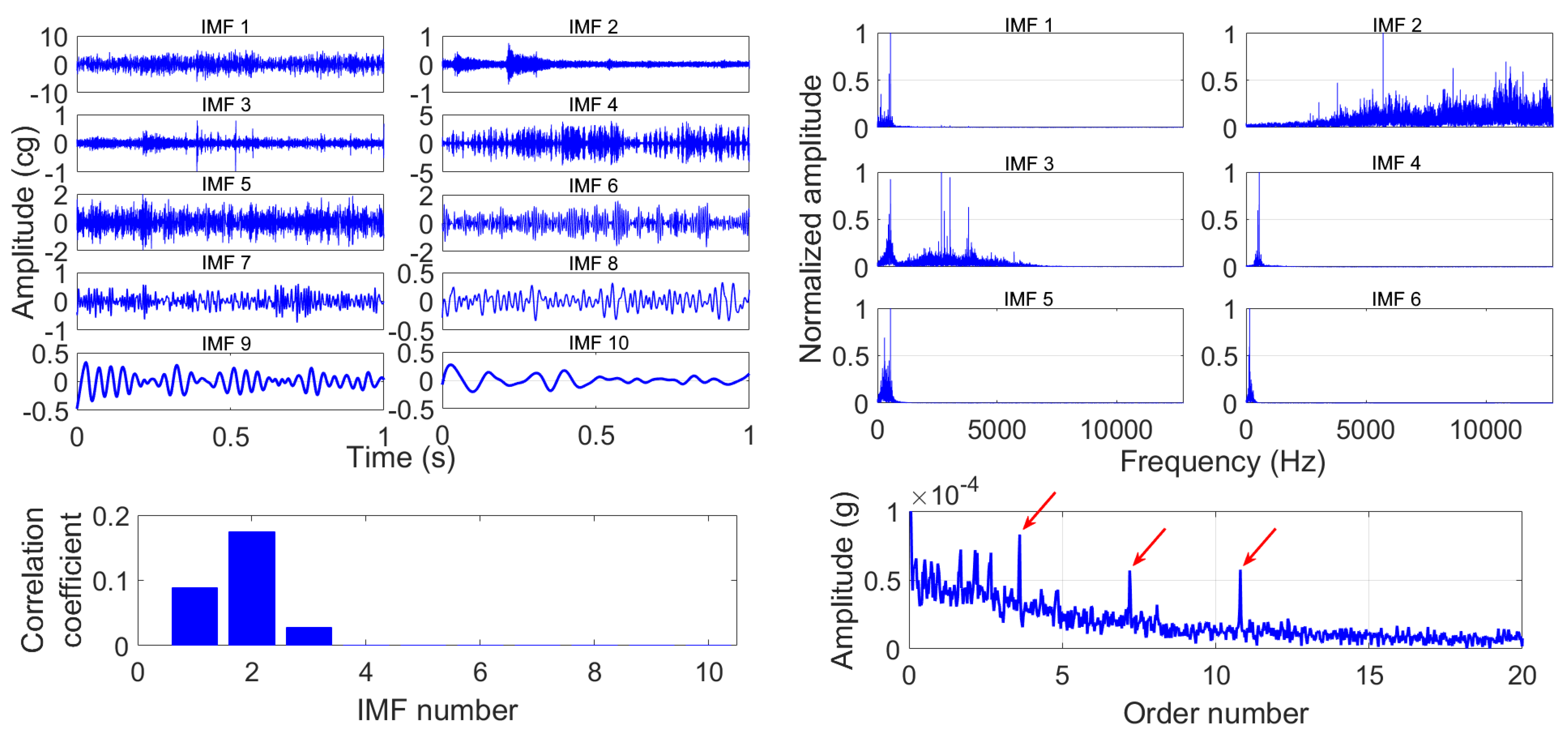
Figure 10.
Sound pressure level meter at the center of the tower.

Table 1.
Acoustic measurements: Turbine 1: sound drive-train, Turbine 2: with bearing fault.
| Turbine 1 | Turbine 2 | ||||||
|---|---|---|---|---|---|---|---|
| No. | Condition | Wind Speed (m/s) | LA (dBA) | No. | Condition | Wind Speed (m/s) | LA (dBA) |
| 1 | Fully OFF | 4.45 | 60.6 | 1 | Fully OFF | 8.23 | 62.1 |
| 2 | WT ON Transformer OFF | 5.37 | 66.82 | 2 | Fully ON | 4.2 | 82.05 |
| 3 | Fully ON | 5.5 | 81.25 | 3 | Fully ON | 8.42 | 82.2 |
| 4 | Fully ON | 8.83 | 81.74 | 4 | Fully ON | 8.9 | 82.5 |
| 5 | Fully ON | 11.93 | 82.16 | ||||
© 2017 by the authors. Licensee MDPI, Basel, Switzerland. This article is an open access article distributed under the terms and conditions of the Creative Commons Attribution (CC BY) license (http://creativecommons.org/licenses/by/4.0/).
Share and Cite
MDPI and ACS Style
Mollasalehi, E.; Wood, D.; Sun, Q. Indicative Fault Diagnosis of Wind Turbine Generator Bearings Using Tower Sound and Vibration. Energies 2017, 10, 1853. https://doi.org/10.3390/en10111853
AMA Style
Mollasalehi E, Wood D, Sun Q. Indicative Fault Diagnosis of Wind Turbine Generator Bearings Using Tower Sound and Vibration. Energies. 2017; 10(11):1853. https://doi.org/10.3390/en10111853
Chicago/Turabian StyleMollasalehi, Ehsan, David Wood, and Qiao Sun. 2017. "Indicative Fault Diagnosis of Wind Turbine Generator Bearings Using Tower Sound and Vibration" Energies 10, no. 11: 1853. https://doi.org/10.3390/en10111853
Note that from the first issue of 2016, this journal uses article numbers instead of page numbers. See further details here.