An Economical Route Planning Method for Plug-In Hybrid Electric Vehicle in Real World
by
 ,
,
Yuanjian Zhang
1, 
Liang Chu
1,
Zicheng Fu
1,
Nan Xu
1,*,
Chong Guo
1,
Yukuan Li
1,
Zhouhuan Chen
2,
Hanwen Sun
2,
Qin Bai
2 and
Yang Ou
2 1
State Key Laboratory of Automotive Dynamic Simulation and Control, Jilin University, Changchun 130022, China
2
China Automotive Engineering Research Institute Co., Ltd, Chongqing 401122, China
*
Author to whom correspondence should be addressed.
Energies 2017, 10(11), 1775; https://doi.org/10.3390/en10111775
Submission received: 24 August 2017
/
Revised: 17 October 2017
/
Accepted: 25 October 2017
/
Published: 3 November 2017
(This article belongs to the Special Issue Energy Management in Vehicle–Grid–Traffic Nexus)
Abstract
:Relieving the adverse effects of automobiles on the environment and natural resources has drawn the attention of numerous researchers. This paper seeks a new path to reach a target by focusing on the synergy of the vehicle and the environment. A real-time economical route planning method for a plug-in hybrid electric vehicle (PHEV) is proposed. Three main contributions have been made. Firstly, a real comparison test is performed to provide rudimentary understanding of the difference in energy usage and route planning between PHEVs and conventional vehicles. Secondly, an approach to obtain PHEV customized data is developed for road weight calculation, which is the essential step in route planning. This method incorporates traffic data from conventional vehicles with the PHEV simulation model, obtaining the required data. Thirdly, the travel expense estimation model (TEEM) is designed. The TEEM could be applied to calculate the road weight of each road segment considering the impact on energy consumption with respect to environmental factors, providing the grounds for route planning. The proposed method to plan an economical route is evaluated, and the results justify its validation and ability to improve fuel economy.
1. Introduction
Resulting from the explosive and unsustainable development of society, the ecological environment has been polluted severely. Among the pollution sources, automobiles contribute greatly [1,2,3,4,5]. In recent years, people have begun to develop new technologies to reduce the adverse effect of automobiles on the environment. Currently, energy-saving and eco-friendly technologies have made significant progress. The proposed methods can improve vehicle fuel economy or exhaust emissions from various aspects, i.e., the vehicle itself, vehicle-environment synergy, etc.
1.1. Literature Review
1.1.1. Technologies Related to the Vehicle Itself
To realize green travel, great efforts have been made in mining the potential of the vehicle itself; for example, improved engine combustion technologies [6,7,8], light weight vehicle technologies [9,10,11], alternative fuel technologies [12,13,14] and hybrid powertrains [15,16,17]. Among the mentioned technologies, hybrid vehicles are seen as one of the reasonable solutions to reduce fuel consumption and exhaust emissions without sacrificing drivability [15,16,17,18,19,20]. Hybrid vehicles can improve fuel economy by taking advantage of multiple power sources and optimal energy management strategies [21,22,23,24]. Amongst hybrid vehicles, plug-in hybrid electric vehicles (PHEVs) have better performance due to being equipped with large capacity batteries and advanced engines [25,26,27,28,29] and, therefore, receiving much attention from researchers.
1.1.2. Vehicle-Environment Synergy Technologies
Thanks to the development of the intelligent transport system (ITS), ubiquitous calculation methods and data mining technologies [30,31,32,33,34,35], some novel solutions to improve vehicle fuel economy and exhaust emissions have appeared. These novel technologies try to solve the problem from the perspective of vehicle and environment synergy [36,37,38]. In these solutions, route planning is one of the effective methods [39,40,41,42,43,44,45]. Route planning is essentially the shortest path problem in graph theory [46]. It is generally acknowledged that the route planning system can be made up of by following sub-modules: digital map, traffic data collection, road weight calculation and route selection. A brief framework of the route planning system is shown in Figure 1, and much research has been performed [47,48,49,50].
The digital map sub-module is mainly in charge of converting the real road network into a digital form, which can be processed by a computer. One of the most preferred tools to generate the digital map is currently MapInfo [51]. The traffic data collection sub-module provides real-time and historical traffic data for route weight calculation. In this sub-module, the collected traffic data include vehicle speed, vehicle geographic data, vehicle fuel consumption, etc. Some mature approaches to collect traffic data have been proposed, i.e., the coil method [52], the video method [53] and the floating car method [54]. Compared with other methods, the floating car method can provide a large number of high quality data while requiring less investment [55]. The route weight calculation sub-module is responsible for calculating the route weight of each route segment. The route weight can be travel time, travel expense, travel fuel consumption, etc. [56]. In the route selection sub-module, some advanced methods, i.e., Dijkstra [57] and A* [58], are applied to identify the shortest route. The Dijkstra algorithm is an efficient method, which can provide the optimal selection result by searching each possible route in the road network. However, the burdensome calculation prevents its real-time application. A* is an algorithm with a fast calculation speed, but it cannot provide the optimal selection result. To guarantee the optimal selection result with real-time application ability, some improvements have been made to the Dijkstra algorithm. The improvements reduce the calculation time by optimizing the storage format of a real road network [59] or by directional result searching [60].
1.2. Motivation and Contribution
According to this study, finding a method to plan an efficient travel route for PHEVs seems meaningful and necessary. When referring to route planning for PHEVs, some challenges are still conspicuous. Ownership of PHEVs is quite low, resulting in the scale of directly-acquired PHEV-specific traffic data being too small to be advantageous in route planning. The energy utilization of PHEVs requires all fuel and electricity consumption to be taken into account. Current portable data collection tools, however, cannot directly and easily log electricity consumption. Moreover, route weight calculation in route planning asks for greater effort. The route weight model that can reveal vehicle performance considering the influence from environment factors may be more meaningful and accurate. The environmental factors can be traffic lights, crossroads, public buildings, surrounding vehicles, etc.
Therefore, according to the discussion, this paper proposes a new real-time method to plan an economical route for PHEVs. Three main contributions have been made in this paper. Firstly, a real comparison test is performed between a PHEV and a conventional gasoline vehicle. The aim of the test is to provide inspiration with regards to the difference in energy usage and route planning between PHEVs and conventional vehicles and to justify the necessity of economical route planning for PHEVs. Secondly, an approach to obtain PHEV customized data is developed. The approach incorporates traffic data of conventional vehicles with the PHEV simulation model. In the PHEV simulation model, a rational energy management strategy is considered to offer performance data for both fuel and electricity. Thirdly, the travel expense estimation model (TEEM) is built to calculate the route weight. The built TEEM can reflect the PHEV energy economy in each route segment considering the impact from the perspective of the environmental factors.
1.3. Outline of the Paper
The reminder of this paper is organized as follows: The real comparison test between a PHEV and a gasoline vehicle is described in Section 2. The real-time economical route planning method for the PHEV is designed in Section 3. The approaches to obtain PHEV customized data and to build the TEEM are specified. Capability analysis of the proposed route planning method is carried out in Section 4, and the conclusions are given in Section 5.
2. Comparison Test between PHEVs and Conventional Vehicles
Compared with conventional vehicles, PHEVs can be driven by two or more different power sources, resulting in various forms of energy utilization. Therefore, it is recommended that there be some preliminary knowledge about PHEVs in regards to energy usage and route planning.
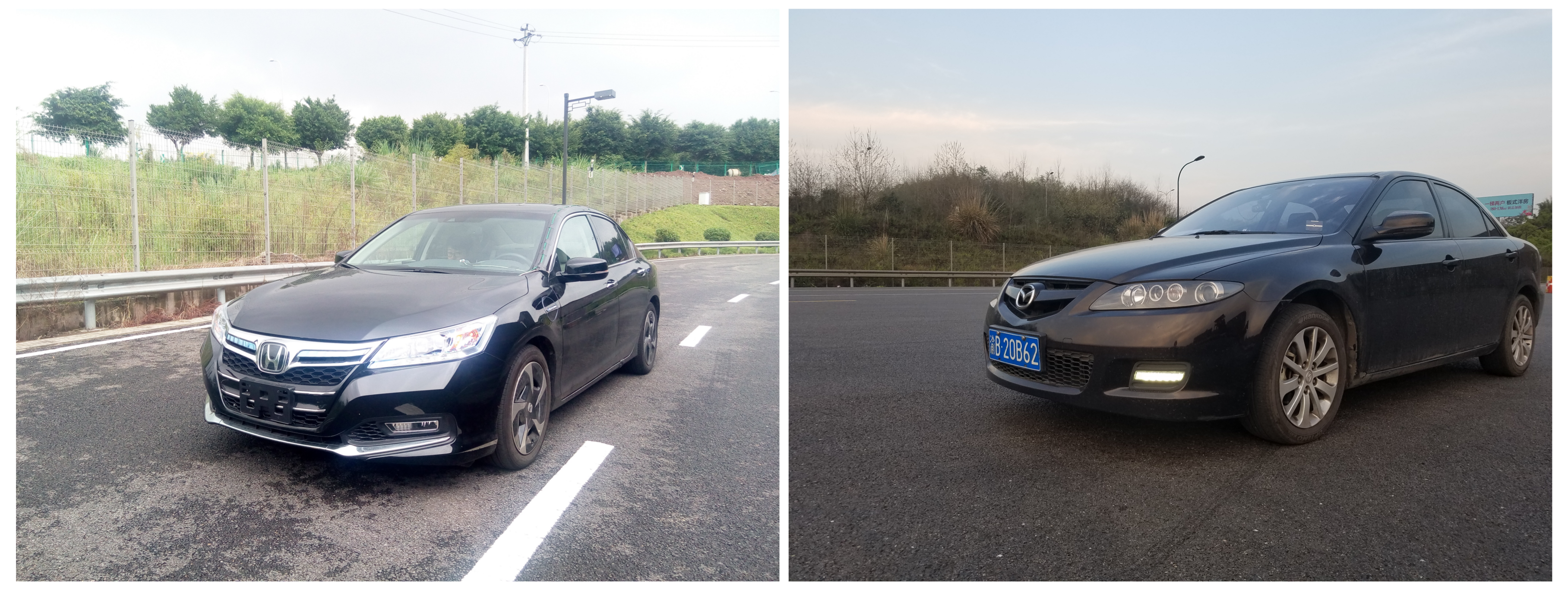
To realize the difference of energy utilization between PHEVs and conventional vehicles intuitively, a real comparison test is performed. The PHEV and gasoline vehicle in the real test are shown in Figure 2. These two vehicles have the same weight with the aid of clump weights, and the engine power is quite close. To accomplish the test, two vehicles are driven by the same driver along two routes (the fastest and shortest route provided by Google Map) at the same time on two different days to ensure the approximate traffic status. The two selected routes are shown in Figure 3, where S means the starting point and D the destination.
While the vehicle is traveling, fuel consumption and electricity consumption (PHEV only) are logged by the OBD (On Board Diagnostics) tool and the power analyzer, respectively, which are shown in Figure 4. According to the data collected in the real test, the energy consumption (fuel and electricity) and travel expense of the two vehicles can be obtained, which is listed in Table 1 and Table 2.
In Table 1 and Table 2, Yuan is the monetary unit of China, and fuel price is that for the testing day. Apparently, the PHEV would have less cost than the gasoline vehicle. When the initial battery SOC is 0.3, for the PHEV, the fuel consumption would be less, and the electricity consumption would be greater in the fastest route than in the shortest route. In this case, traveling the fastest route results in less travel expense and better fuel economy. For the gasoline vehicle, however, the shortest route is recommended. When the initial battery SOC is 0.8, on the contrary, the shortest route is favored for the PHEV, which is the same case as for the gasoline vehicle. Under this case, the engine of the PHEV did not operate for the whole trip, and the travel expense was only determined by electricity consumption.
According to the travel expense comparison between the PHEV and gasoline vehicle, some points can be summarized:
- The difference in energy consumption and travel expense in the two routs reveals that the environment can be a critical element that affects energy consumption, which is considered as the essence of route planning to a certain degree.
- PHEVs hold great potential in fuel economy improvement. With route planning, the potential of PHEVs in travel expense and fuel economy improvement can be fully extended.
- PHEVs can be driven by two power sources. When estimating travel expense or total energy consumption, the energy output of the two power sources should be considered simultaneously. Therefore, the energy management strategy should be known beforehand to make the estimation.
- Different forms pf energy utilization in PHEVs and conventional vehicles lead to the route planning being specially designed for PHEVs.
Energy management strategies in PHEVs govern the energy distribution between engines and batteries. Current energy management strategies applied in PHEVs can be divided into three types: heuristic methods [61,62,63], instantaneous control methods [64,65,66] and global optimization methods [67,68,69]. Global optimization methods require a priori knowledge about the driving cycle, which cannot be applied in real time. Heuristic methods can be applied in real time easily, while they are lacking the optimal control effect. Instantaneous control methods can be applied in real time and possess reasonable performance, which are gradually being accepted by engineering practice [70]. Some instantaneous control methods have been proven that can offer the optimal energy management effect close to global optimization methods [71]. As the route planning is more of a real-time process, instantaneous control methods are suggested when developing the route planning method for PHEV.
Based on the real test, we realize the potential of PHEVs in travel expense saving and fuel economy improvement, understand the difference in route planning between PHEVs and conventional vehicles and comprehend the influence on route planning from the forms of energy utilization of PHEVs. In the next step, we will focus on the route planning method for PHEVs accordingly.
3. Real-Time Economical Route Planning for PHEVs
Generally, the route planning process can be described as follows: firstly, collecting traffic data (historical and instantaneous) for route weight calculation; secondly, calculating the route weight of each route segment based on the digital map and the traffic data collected; finally, picking the optimal route via a certain algorithm.
Owing to the special features of PHEVs, traffic data collection and route weight calculation are the main innovations in the proposed method, which will be discussed in detail. The digital map is formed by MapInfo (Pitney Bowes, Stamford, CT, USA) [51], and the details of digital map generation can be seen in [72]. The economical route is picked by the Dijkstra algorithm. To guarantee real-time application, some improvements should be made to the Dijkstra algorithm. To begin with, the road network storage format is changed into an adjacency list from the adjacency matrix, the details of which are in [59]. As a result, the computational complexity is reduced to from . Then, the search area of the candidate routes is narrowed by the rectangle limit method [60]. The rectangle limit method accomplishes the search for the directional candidate, reducing the burden of the calculation. Finally, the shortest route and the fastest route are a priori chosen first, and then, the economical route for the PHEV is determined between the shortest route and the fastest route. The shortest route and the fastest route can be obtained with few calculations due to the easily calculated route weight without considering the energy consumption of fuel and electricity. In addition, energy consumption is highly related to the route length and travel time [73]. A shorter travel length requires less tractive energy, and faster travel may not result in greater acceleration resistance, which is a benefit to fuel savings. Besides, the operation of the PHEV can be divided into two stages according to the state of the battery. In particular, it would be in the CDstage if the battery SOC were greater than 0.28 and in the CSstage if the battery SOC were less than 0.28. In the CD stage, the battery would be the primary source to drive the vehicle, and the engine only outputs energy for the large tractive power requirement. In the CS stage, the battery discharge ability is abated significantly, and the engine would drive the vehicle for most of the time. The combination of the CD and CS stages realizes the optimal fuel economy and the ideal travel mileage. Besides, the TEEM takes the different operation stages into account when planning the economical route, making sure the fuel economy can be optimal in both the CD and CS stages. Hence, the vehicle does not need take a detour elsewhere to charge, instead of following the optimal route, when the battery SOC is low. A detour would most likely occur in purely electric vehicles.
3.1. PHEV Customized Traffic Data Collection
As is described, the floating car method is chosen as an ideal method to collect traffic data. The floating car-based method for route planning is the statistical calculation using the shared data from all volunteering vehicles on route segments rather than a certain floating car. Therefore, the economical route is picked according to the general situation of the route segments, avoiding route segments with heavy traffic due to the same decision of different cars. The floating car method can be divided into the following steps, which are illustrated in Figure 5.
According to Figure 5, OBD scanners and GPS units are applied to collect the traffic data of volunteering vehicles. Traffic data include real-time geographic coordinates, speed, time stamp, fuel consumption, etc. The gathered traffic data are transferred to the information processing terminal in the cloud. User terminals (mobile phones, etc.) would plan the route taking into consideration the requirements of the drivers. To solve the shortage of original PHEV customized traffic data, we incorporate the simulation technology with the traffic data that belong to conventional vehicles. In this solution, velocity sequences parsed from conventional floating car data are input into the simplified PHEV model first. Then, PHEV customized traffic data that include the performance with respect to fuel and electricity can be acquired. This method can make sense of the vehicle speed distribution in real roads, which tends to be same for PHEVs and conventional vehicles. In the built model, the energy management strategy is included to provide the data of the fuel and electricity.
3.1.1. PHEV Powertrain Model
A simplified vehicle model is built, which aims to reflect the longitudinal performance of the PHEV in real time. In this paper, the parallel PHEV is taken as an example.
Vehicle Longitudinal Dynamic Model
The driving requirements are provided by the driver. The required tractive force necessary to drive vehicle can be expressed as:
where G, and f are gravity, gradient and the rolling resistance factor, respectively; , A and v are the aerodynamic drag factor, frontal area and vehicle speed, respectively. The required tractive torque at the wheel can be calculated as:
where is wheel radius, a is acceleration and is the moment of inertial. At the wheel, the torque balance equation can be written as:
where is torque generated from the fuel and is the torque produced from the electricity.
Fuel Model
In the fuel model, the basic relationships can be expressed as:
where is engine torque; and are the engine and wheel angular velocity, respectively; and are the gear and final drive ratio, respectively; n is the gear number; is the transmission efficiency of the fuel.
Electricity Model
The relationship applied in the electricity model can be expressed as:
where is the motor torque, is the motor angular velocity and is the transmission efficiency of the electricity.
For the battery, the relationship used for evaluating the battery current and battery SOC is included in the following equation:
where is the battery open circuit voltage, is the battery internal resistance and is the battery power. The battery SOC can be expressed as:
where is the maximum capacity.
3.1.2. Energy Management Strategy
In this paper, the optimization goal of energy management is fuel economy. The cost function of the optimization problem can be written as:
where is the fuel mass flow rate, is the energy density of the fuel, t is discrete time, is the time interval, is the energy consumed by the vehicle and s is the equivalent factor. In Equation (10), can be calculated as:
where is the fuel’s lower heating value, is the required engine power and is the engine efficiency at that moment. can be written as:
where is the required instantaneous longitudinal tractive energy and u is the power split ratio between the engine and battery. The control function for minimizing their instantaneous equivalent fuel consumption can be written as:
where is the optimal power split ratio.
Generally, the equivalent factor comprises various parameters influenced by many factors, i.e., future driving conditions, components’ status, etc. For energy management, positive battery power (discharge) means some electric energy should be replenished in the future by the engine or the grid, causing an extra equivalent factor for fuel to be added; negative battery power (charge) signifies that some electric energy can be saved for future consumption, saving some equivalent fuel. Hence, the current policy for the power distribution may result in some extra energy consumption. How much equivalent fuel would be required to replenish electric energy or how much can be saved depends on the operation status of the components affected by future driving conditions. As a result, the equivalent factor should be tuned accordingly. In this paper, the equivalent factor is adjusted by the method in our former work in [74]. After collecting enough PEHV customized traffic data, the route weight of each route segment can be calculated.
3.2. TEEM Building
TEEM is applied to calculate the route weight of each route segment. In this paper, the route weight is the estimated travel expense (ETE). Actually, TEEM includes three steps: firstly, calculating the required instantaneous longitudinal tractive energy; secondly, determining the required energy from the fuel and electricity by the energy management strategy; thirdly, consequently obtaining ETE. The three steps are illustrated in Figure 6.
Step 1: Required Instantaneous Longitudinal Tractive Energy Calculation
The required instantaneous longitudinal tractive energy can be calculated by Equation (14). In Equation (14), is the correction coefficient of rotating mass, and a is acceleration.
Equation (14) is a generally accepted method to calculate the required instantaneous longitudinal tractive energy. However, some improvements can be made in this paper. Two reasons are provided for the improvement. On the one hand, the vehicle speed in Equation (14) is provided by the floating car method. However, the floating car method only offers the average speed of the route segment. As a result, Equation (14) actually reflects the average energy consumption level of a certain route segment. Hence, positive instantaneous speed benefits accurate calculation. On the other hand, in Equation (14) is the acceleration resistance. As a matter of fact, acceleration resistance is influenced by environmental factors. The impact from environmental factors can be further explained by the following example. When drivers are driving vehicles passing by a school, they may actively decelerate for safety reasons and then accelerate. Frequently, acceleration and deceleration are affected by environmental factors, which cause the variation of acceleration resistance and extra energy consumption. Therefore, it may provide more precise and rational acceleration resistance if acceleration calculation considers the impact if environmental factors.
According to the analysis, a revised method is applied to calculate velocity and acceleration, making more reasonable. It is requested that the impact of surrounding vehicles on the fuel economy be considered. Microscopic traffic flow theory models, i.e., Gazis, Edie and Newell, seem to be appropriate for their advantages in describing the relationship between individual vehicles and surrounding vehicles [75]. The Edie model, as a kind of microscopic model, has been widely accepted and is easily applied in real time [76]. The Edie model can be expressed as:
where is the sensitivity coefficient, M is vehicle mass and is the lag time of the driver-car system. In addition, x represents the vehicle position. Solving Equation (15), we can get:
where is unimpeded velocity, is jam density and is the real-time density of traffic flow. In Equation (16), is a constant value determined by the route conditions, which can be acquired from the digital map. The density of traffic flow can be calculated by the following equation:
where q is the flow of a certain route segment and is the average speed of the vehicle on a certain route segment, which can be calculated as follows:
where and n are the instantaneous speed of a floating car and the number of floating cars sitting on a certain route segment, respectively. The flow can be expressed as follows:
where is the average headway, which is the time lag for which identical components in adjacent vehicles pass the same point. Therefore, Equation (16) can be rewritten as:
Then, by the formula of Tailor, Equation (20) is changed into the following equation, which is the third order expansion with reasonable calculation accuracy and computation [77]:
Therefore, instantaneous acceleration can be acquired by taking derivative of Equation (21), which is shown in Equation (22).
where is the average acceleration of a certain route segment, which can be calculated be the following equation:
where , is the average speed of a certain route segment and the previously adjacent route segment, respectively; is time of travel from the midpoint of the previously adjacent route segment to the current one, which can be calculated as:
where is the length of two route segments, respectively.
In Equation (21), and are variables influenced by environment factors from both sides of the route, such as traffic lights, neighboring route segments, public buildings, i.e., schools, hospitals, gas stations, etc., entertainment buildings, i.e., shopping malls and theaters, surrounding vehicles, etc. Hence, can be replaced by the following equation:
where , , and are the number of traffic lights, neighboring route segments, public buildings and entertainment buildings in a certain route segment, respectively.
Together with Equations (23)–(26), the required instantaneous longitudinal tractive energy can be acquired by taking Equations (21) and (22) into Equation (14). To allow TEEM to become a general mode and be applied in real time, constant parameters should be derived. In the parameter derivation, historical PHEV customized traffic data are obtained by the method in Section 3.1; and can be extracted from the OpenStreetMap (OpenStreetMap Foundation, Sutton Coldfield, UK) (OSM) platform [78]. These data are employed to derive by the linear regression method [79].
Step 2: Energy Distribution
To estimate the travel expense of PHEV, the energy consumptions of fuel and electricity should be considered together. After obtaining the required instantaneous longitudinal tractive energy in Step 1, the required instantaneous energy provided by fuel and electricity can be determined by the energy management strategy. ECMSis adopted again to acquire the optimal energy distribution.
Step 3: ETE Acquisition
In general, ETE is the integration of the instantaneous travel expense (ITE) in each route segment. The ITE can be calculated as:
where and are the price unit of fuel (gasoline) and electricity, respectively; is the fuel density. According to Equation (11), the ITE function can be rewritten as:
In Equation (28), and can be gained in Step 2. As a result, ETE can be expressed as:
where is the time when the PHEV enters and leaves the given route segment, which can be written as:
4. Capability Analysis of the Proposed Route Planning Method
In this section, some evaluations are performed. Firstly, the accuracy of the simulation model is tested to figure out if it can be used to prepare the PHEV-specific traffic data. Secondly, the performance of TEEM is analyzed to check the capability of TEEM in route planning. Thirdly, the effect of economical route planning is estimated to justify the potential of the proposed method in travel expense savings and fuel economy improvement. In this paper, the traffic data of conventional vehicles are contributed by floating cars in Beijing, China, during the period of 2 February–8 February 2008.
4.1. Evaluation of the Simulation Model
To guarantee that the obtained traffic data are reasonable and have acceptable accuracy to reflect the PHEVs’ real energy consumption, the simulation model needs to have high precision. The evaluation of simulation model is divided into two parts. In the first part, the simulation model is evaluated by comparing the vehicle velocity difference between the simulation result and the real vehicle velocity sequence. The real vehicle velocity sequences are input into eight simulation models, which correspond to eight PHEVs. The eight corresponding PHEVs are all parallel PHEVs, and their basic information is listed in Table 3. The comparison results of the two types of velocity sequences is listed in Table 4.
The results in Table 4 are the average degree of eight PHEV models after running the simulation on 20 chosen routes with different vehicle velocity sequences. It can be seen that the simulation model accuracy is 98.1% when the velocity difference is less than 2 m/s, and the simulation model accuracy is 99.9% when the velocity difference is less than 4 m/s. According to the comparison results, it can be concluded that the basic capability of the simulation model is reasonable.
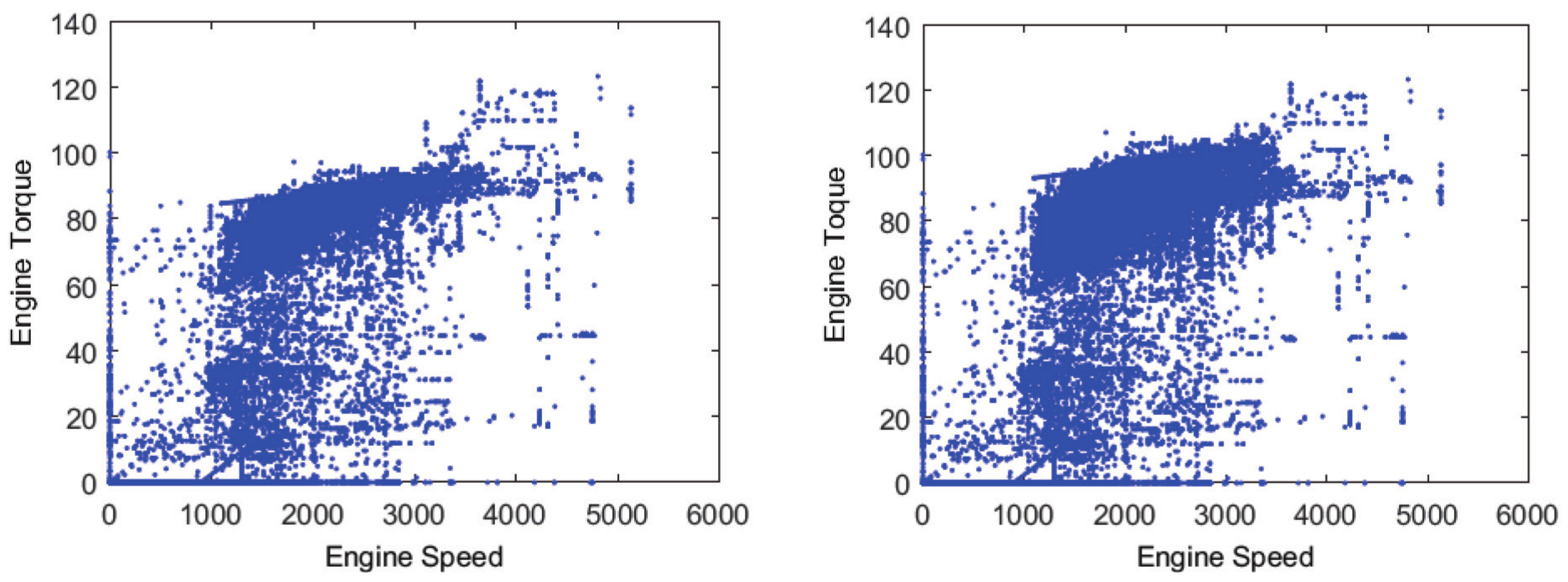
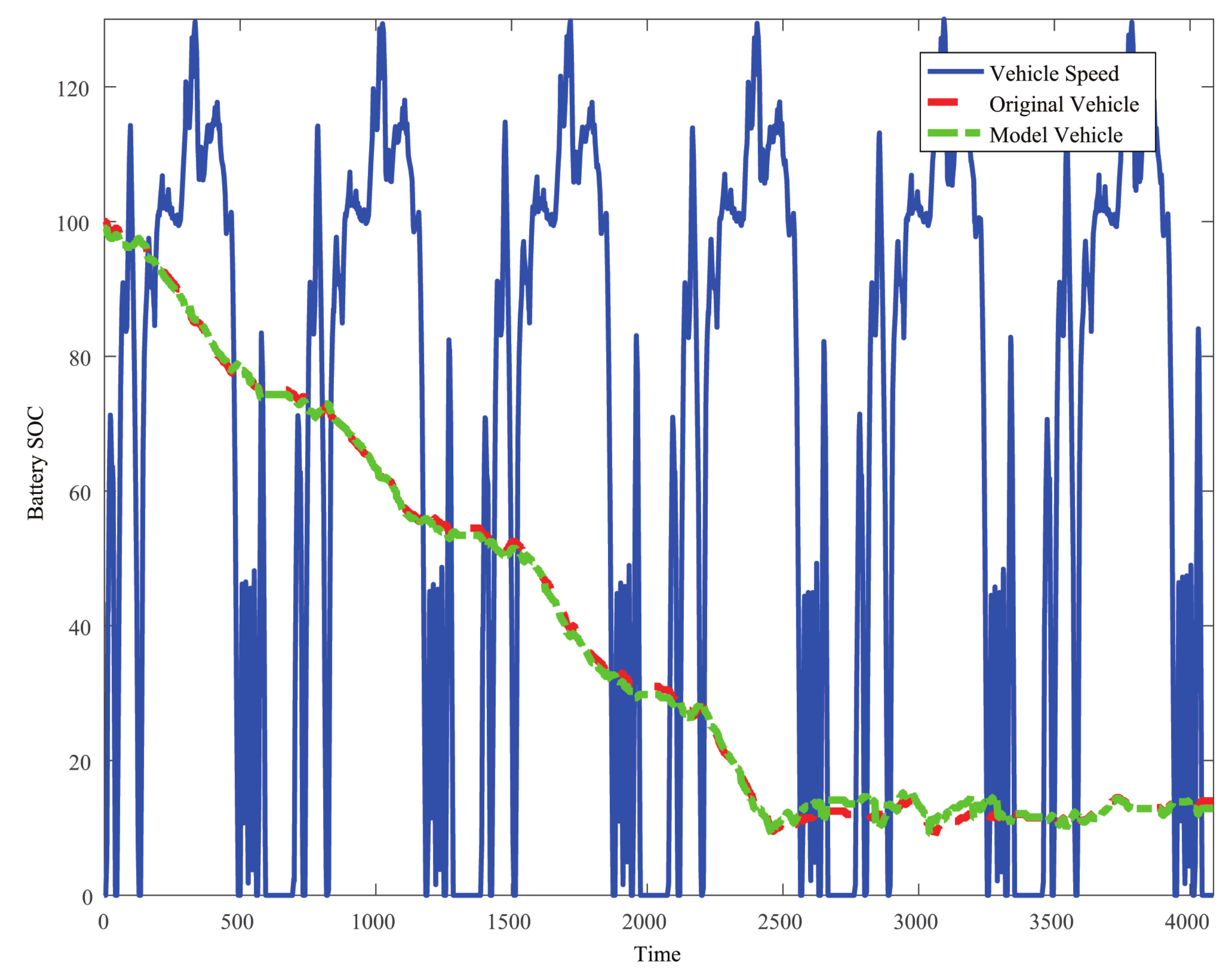
In the second part, the simulation model is investigated more deeply. We made the benchmark test on the Hyundai Sonata PHEV, picked from the eight PHEVs, based on the dynamometer, acquiring the component performance. Then, we compare the operation status of the components from the simulation and benchmark test. Figure 7 and Figure 8 reveal the engine and motor operating points in several standard testing cycles, respectively. Figure 9 reveals the battery performance in the US06 standard testing cycle.
According to Figure 7, Figure 8 and Figure 9, the components’ performance from the simulation is quite close to that from the benchmark test. To be specific, the engine operation points and motor operation points are all slightly less concentrated in the simulation than those in the benchmark test, meaning the vehicle fuel economy in the simulation may be mildly worse than the real vehicle. The mean squared error of the engine operation points in the benchmark test is 29.74, while it is 35.63 in the simulation. Similarly, the mean squared error of the motor operation points in the benchmark test is 45.61, while it is 47.14 in the simulation. However, the gap in the engine and motor performance between the simulation and benchmark test is quite narrow. Similarly, despite that there is a difference in the battery SOC between the simulation and the benchmark test, the difference is quite small, and the total variation trend is quite similar. The comparison between the results from the simulation and the benchmark test justifies that the simulation model built can provide reasonable data with acceptable accuracy.
4.2. Evaluation of TEEM
Just like the evaluation in Section 4.1, the performance of TEEM is investigated by comparing the travel expense estimated by TEEM to the real expense offered by the simulation model and acquired in the real test. The error between the estimated travel expense and the real travel expense is calculated by the following equation:
where is the estimated travel expense of a certain route provided by TEEM and is the real travel expense.
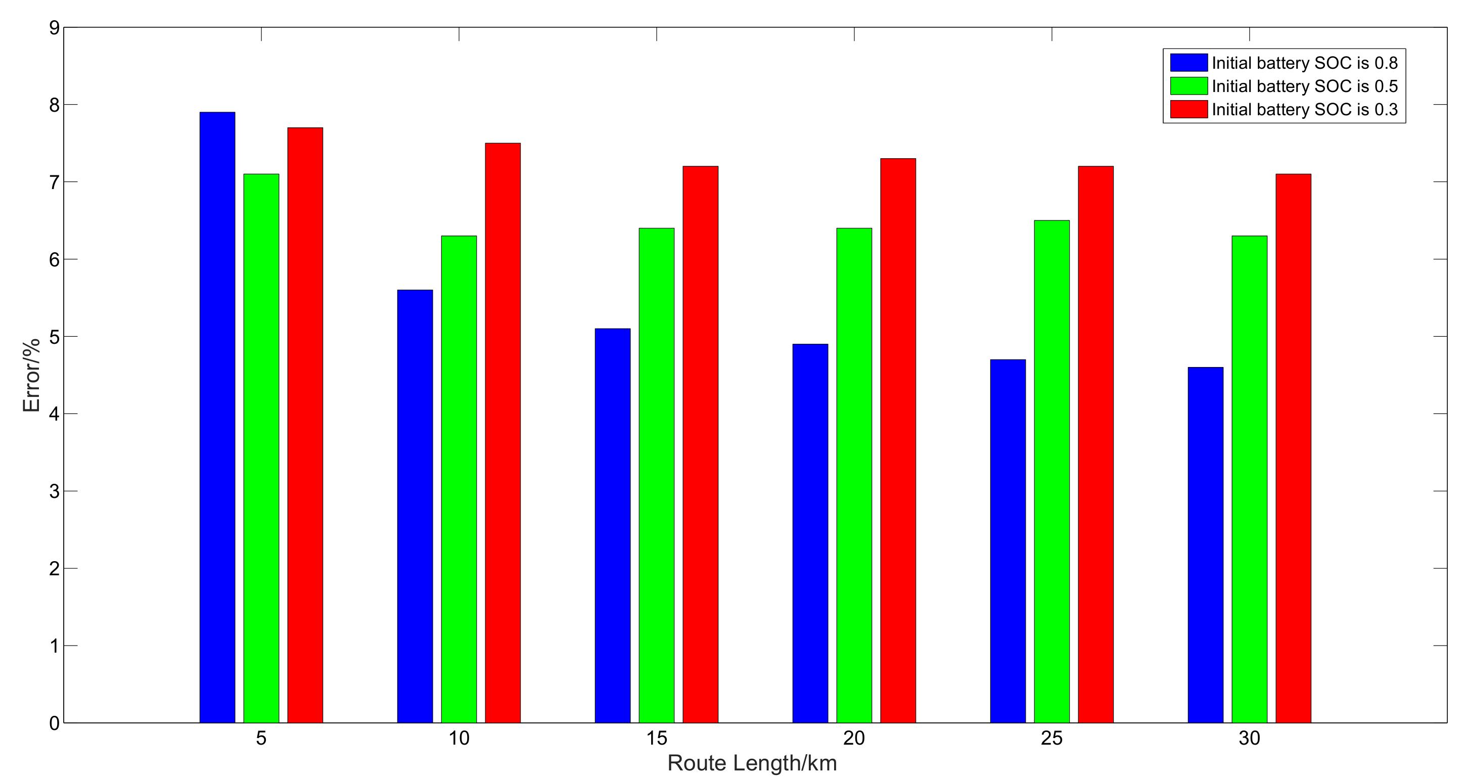
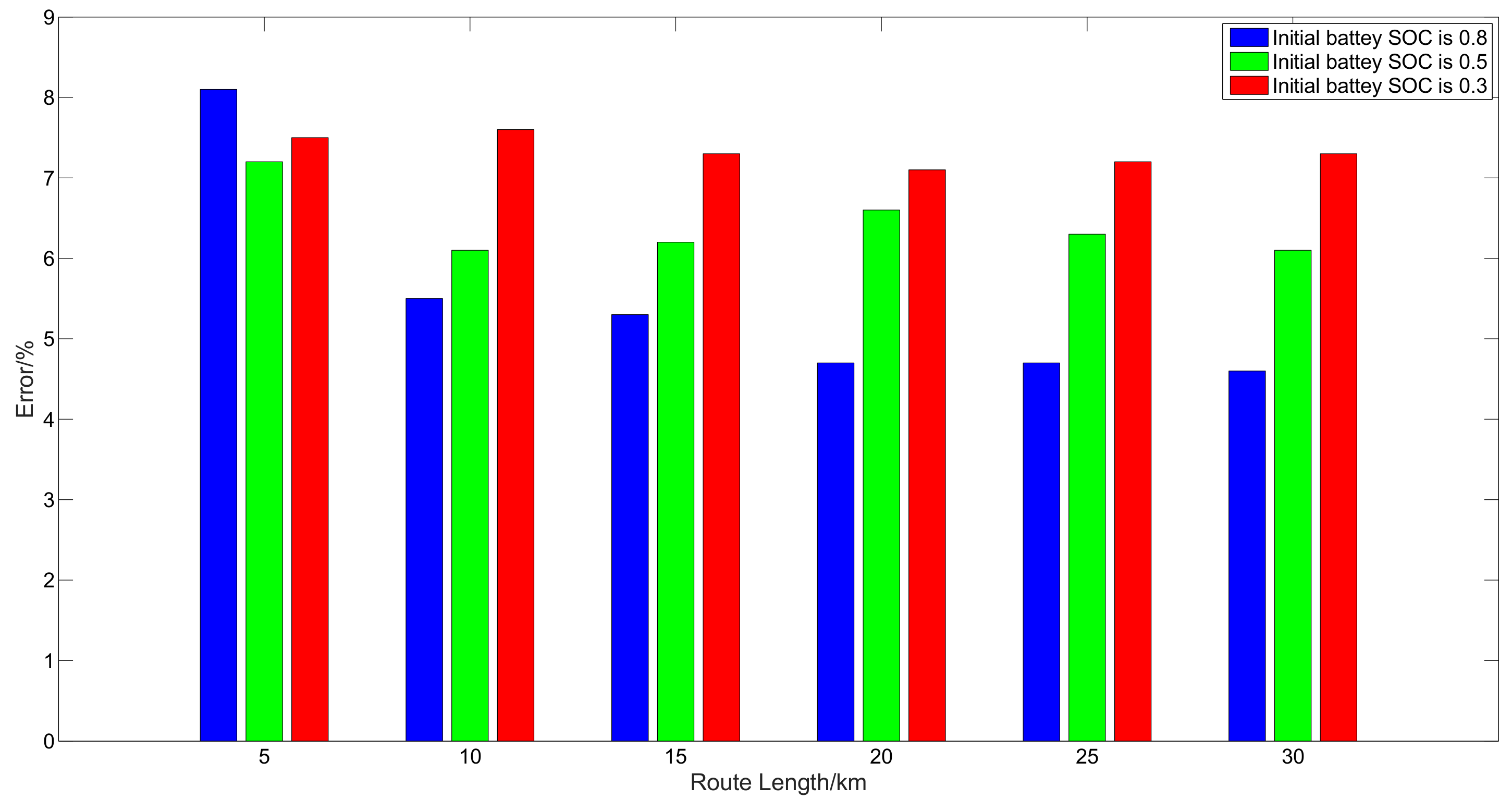
Figure 10 and Figure 11 provide the evaluation results between the estimated travel expense by TEEM and the real expense by the simulation model. Figure 10 reveals the TEEM accuracy when a PEHV (No. 1 in Table 3) drives on routes with different lengths and various initial battery SOCs. Figure 11 illustrates the TEEM performance to estimate different PHEVs’ travel expense with various initial battery SOCs when the route length is 10 km. In Figure 11, most errors of TEEM in the travel expense estimation are below 10%, which is an acceptable value [73]. The error of TEEM is determined by multiple aspects, i.e., unbalanced distribution of floating car data, the error of the simulation model and TEEM training error. In this paper, it is accepted if the error is less than 10%. Generally, the TEEM accuracy would improve with the route length increasing for a larger quantity of floating car data. Different initial battery SOCs actually reflect the various operation modes of the PHEV. In particular, when the initial SOC is 0.8, the PHEV would operate in the CD stage, and the accuracy is better than others. The motor would drive the vehicle for most of the time. The motor, as a component with small inertia, can respond to the tractive requirement quickly in the simulation model, ensuring less error. When the initial SOC is 0.3, the vehicle would be in the CS stage, and the engine would be the primary power source. The engine, as a component with large inertia, cannot respond to the tractive requirement quickly, increasing the TEEM training and prediction error. Figure 12 presents the comparison results between the estimated travel expense by TEEM and the expense from the real test. In the real test, we employ our benchmark vehicle (No. 1 in Table 3). The vehicle is driven by the same driver along the routes, leading to results in Figure 10, obtaining the error between estimated TEEM and the real travel expense. Accordingly, the errors between TEEM and the real travel expense are also less than 10% and quite close to those in Figure 10. The results in Figure 12 justify the accuracy of TEEM and the simulation model.
4.3. Evaluation of Route Planning
After performing the evaluation of the simulation model and TEEM, this section mainly deals with the potential in travel expense savings and fuel economy improvement of the proposed route planning method. In this evaluation, three travel routes were chosen by the proposed method in Section 3 under different initial battery SOCs after a given start point and destination. In the three travel routes, one is the recommended route with the minimum travel expense, and the other is the shortest or the fastest route. The third route is called the optional route, which is chosen to contrast. The optional route is picked according to the floating car distribution. In the chosen optional route, the quantity of floating cars is quite large, which leads to the assumption that people tend to travel along this route. In the evaluation, the fuel price is that for the traffic data date.
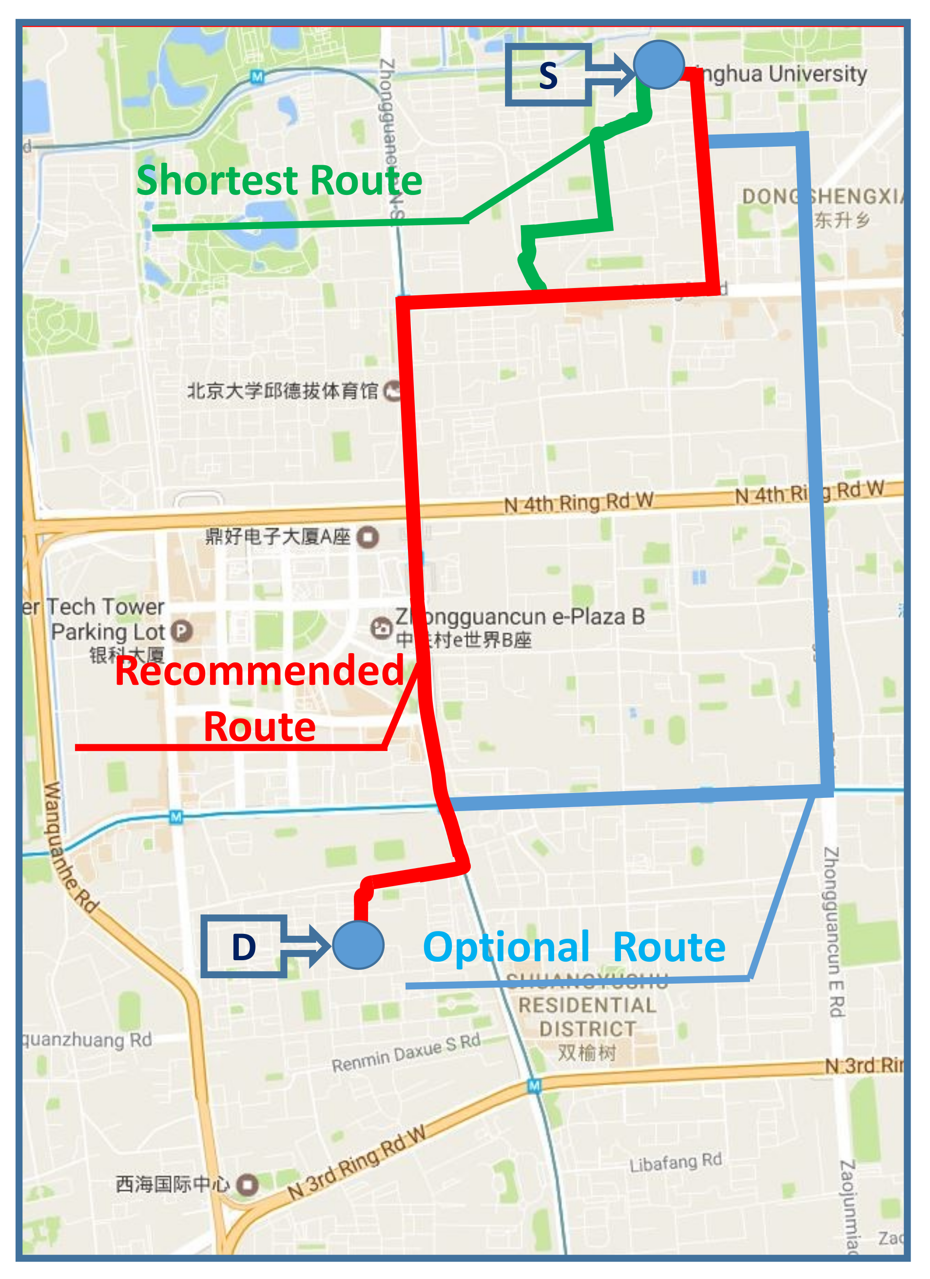
When the initial battery SOC is 0.3, the route map is as shown in Figure 13. The energy consumption and travel expense of the PHEV are listed in Table 5.
In Table 5, the PEHV would consume less fuel and possess the minimum travel expense when it travels along the recommended (fastest) route.
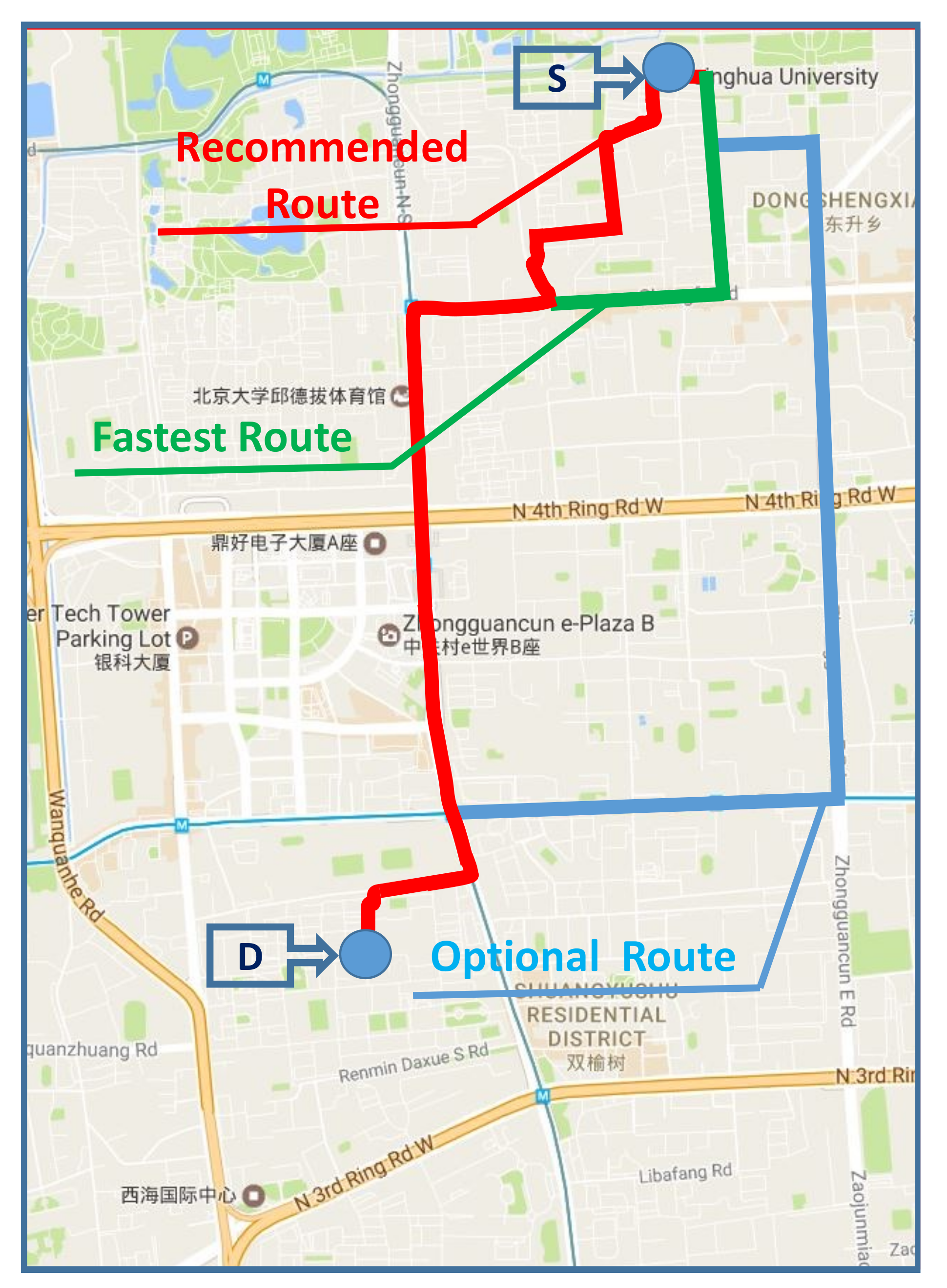
When the initial battery SOC is 0.8, three routes are also picked, and the routes’ map is shown in Figure 14. As is listed in Table 6, the fuel consumption is zero when the initial battery SOC is 0.8; this is because the PHEV in the CD stage would be driven by the battery according to the energy management strategy. More importantly, the recommended route is the shortest route, which is different from that when the initial battery SOC is 0.3.
Through the investigation, it can be justified that the proposed route planning method can offer the travel path with the minimum travel expense and ideal fuel economy. Moreover, the difference in the recommended routes when the initial battery SOC is varied also demonstrates that the PHEV’s forms of energy utilization make the route planning much more complicated.
5. Conclusions
In this paper, we come up with a method to plan an economical route for PHEVs. The evaluation results justify that the method has the capability to improve the fuel economy to some degree. Two main works have been performed. Firstly, we innovatively solved the shortage of PHEV customized traffic data. Traffic data from conventional vehicles and the PHEV simulation model are incorporated, obtaining PHEV-specific traffic data for route weight calculation. Secondly, TEEM is developed based on microscopic traffic flow theory with the consideration of the effect of the environment on the energy consumption.
In future research, we want to carefully investigate the environmental factors that can influence the PHEV energy consumption and to build a more accurate and general TEEM. In addition, we will try to take the driving behavior factors into account when designing TEEM.
Acknowledgments
This paper is supported by: 1. China Postdoctoral Science Foundation(2014M561290); 2. Energy Administration of Jilin Province [2016]35; 3. Jilin Province Science and Technology Development Funds (20150520115JH).
Author Contributions
Yuanjian Zhang, Liang Chu, and Nan Xu proposed the method to plan the most economical route for the PHEV. Zicheng Fu checked the manuscript and helped to build the Simulink model. Chong Guo, Yukuan Li, Zhouhuan Chen, Hanwen Sun, Yang Ou and Qin Bai checked the manuscript.
Conflicts of Interest
The authors have no conflicts of interest.
Nomenclature
| f | rolling resistance factor | m | vehicle mass |
| G | gravity acceleration | road gradient | |
| air drag coefficient | A | vehicle frontal area | |
| v | vehicle speed | required tractive torque | |
| wheel radius | a | acceleration | |
| moment of inertia | torque generated from fuel | ||
| torque produced from electricity | engine torque | ||
| engine angular velocity | wheel angular velocity | ||
| gear ratio | final drive ratio | ||
| n | gear number | transmission efficiency of fuel | |
| motor torque | motor angular velocity | ||
| transmission efficiency of electricity | battery power | ||
| battery open circuit voltage | battery internal resistance | ||
| battery maximum capacity | fuel mass flow rate | ||
| energy density of fuel | t | discrete time | |
| time interval | energy consumed by vehicle | ||
| s | equivalent factor | fuel lower heating value | |
| required engine power | engine efficiency | ||
| required instantaneous longitudinal tractive energy | u | power split ratio | |
| optimal power split ratio | correction coefficient of rotating mass | ||
| sensitivity coefficient | lag time | ||
| x | vehicle position | unimpeded velocity | |
| jam density | density of traffic flow | ||
| q | flow of a certain route segment | average speed of vehicle on a certain route segment | |
| instantaneous speed | n | number of floating cars | |
| average headway | average acceleration of the vehicle on a certain route segment | ||
| travel time on two adjacent route segments | length of the route segment | ||
| number of traffic lights | number of neighboring route segments | ||
| number of public buildings | number of traffic lights | ||
| price unit of fuel | price unit of electricity | ||
| fuel density |
References
- Chen, S.M.; He, L.Y. Welfare loss of China’s air pollution: How to make personal vehicle transportation policy. China Econ. Rev. 2014, 31, 106–118. [Google Scholar] [CrossRef]
- Zhang, K.; Batterman, S. Air pollution and health risks due to vehicle traffic. Sci. Total Environ. 2013, 450, 307–316. [Google Scholar] [CrossRef] [PubMed]
- He, H.; Wang, Y.; Ma, Q.; Ma, J.; Chu, B.; Ji, D.; Tang, G.; Liu, C.; Zhang, H.; Hao, J. Mineral dust and NOx promote the conversion of SO2 to sulfate in heavy pollution days. Sci. Rep. 2014, 4, 4172. [Google Scholar] [CrossRef] [PubMed]
- Zhang, H.; Wang, S.; Hao, J.; Wang, X.; Wang, S.; Chai, F.; Li, M. Air pollution and control action in Beijing. J. Clean. Prod. 2016, 112, 1519–1527. [Google Scholar] [CrossRef]
- Li, Q.; Qiao, F.; Yu, L. Will Vehicle and Roadside Communications Reduce Emitted Air Pollution? Int. J. Sci. Technol. 2015, 5, 17–23. [Google Scholar]
- Agarwal, A.K.; Srivastava, D.K.; Dhar, A.; Maurya, R.K.; Shukla, P.C.; Singh, A.P. Effect of fuel injection timing and pressure on combustion, emissions and performance characteristics of a single cylinder diesel engine. Fuel 2013, 111, 374–383. [Google Scholar] [CrossRef]
- Sajjad, H.; Masjuki, H.; Varman, M.; Kalam, M.; Arbab, M.; Imtenan, S.; Rahman, S.A. Engine combustion, performance and emission characteristics of gas to liquid (GTL) fuels and its blends with diesel and bio-diesel. Renew. Sustain. Energy Rev. 2014, 30, 961–986. [Google Scholar] [CrossRef]
- Kong, S.C.; Marriott, C.D.; Reitz, R.D.; Christensen, M. Modeling and Experiments of HCCI Engine Combustion Using Detailed Chemical Kinetics with Multidimensional CFD; Technical Report; SAE Technical Paper; SAE World Congress: Detroit, MI, USA, 2001. [Google Scholar]
- Kim, H.C.; Wallington, T.J.; Sullivan, J.L.; Keoleian, G.A. Life Cycle Assessment of Vehicle Lightweighting: Novel Mathematical Methods to Estimate Use-Phase Fuel Consumption. Environ. Sci. Technol. 2015, 49, 10209–10216. [Google Scholar] [CrossRef] [PubMed]
- Bubna, P.; Wiseman, M. Impact of Light-Weight Design on Manufacturing Cost—A Review of BMW i3 and Toyota Corolla Body Components; Technical Report; SAE Technical Paper; SAE World Congress and Exhibition: Detroit, MI, USA, 2016. [Google Scholar]
- Seyfried, P.; Taiss, E.J.M.; Calijorne, A.C.; Li, F.P.; Song, Q.F. Light weighting opportunities and material choice for commercial vehicle frame structures from a design point of view. Adv. Manuf. 2015, 3, 19–26. [Google Scholar] [CrossRef]
- Chen, L.; Zhang, J.; Li, Y.; Ye, Y. Mechanism analysis and evaluation methodology of regenerative braking contribution to energy efficiency improvement of electrified vehicles. Energy Convers. Manag. 2015, 92, 469–482. [Google Scholar]
- Koetse, M.J.; Hoen, A. Preferences for alternative fuel vehicles of company car drivers. Resour. Energy Econ. 2014, 37, 279–301. [Google Scholar] [CrossRef]
- Lee, S.; Speight, J.G.; Loyalka, S.K. Handbook of Alternative Fuel Technologies; CRC Press: Boca Raton, FL, USA, 2014. [Google Scholar]
- Hu, X.; Murgovski, N.; Johannesson, L.M.; Egardt, B. Comparison of three electrochemical energy buffers applied to a hybrid bus powertrain with simultaneous optimal sizing and energy management. IEEE Trans. Intell. Transp. Syst. 2014, 15, 1193–1205. [Google Scholar] [CrossRef]
- Lv, C.; Zhang, J.; Li, Y.; Yuan, Y. Directional-stability-aware brake blending control synthesis for over-actuated electric vehicles during straight-line deceleration. Mechatronics 2016, 38, 121–131. [Google Scholar] [CrossRef]
- Sockeel, N.; Shi, J.; Shahverdi, M.; Mazzola, M. Sensitivity analysis of the battery model for model predictive control implemented into a plug-in hybrid electric vehicle. In Proceedings of the 2017 IEEE Transportation Electrification Conference and Expo, Chicago, IL, USA, 22–24 June 2017; pp. 493–500. [Google Scholar]
- Zhang, J.; Lv, C.; Gou, J.; Kong, D. Cooperative control of regenerative braking and hydraulic braking of an electrified passenger car. Proc. Inst. Mech. Eng. Part D J. Automob. Eng. 2012, 226, 1289–1302. [Google Scholar] [CrossRef]
- Heutel, G.; Muehlegger, E. Consumer learning and hybrid vehicle adoption. Environ. Resour. Econ. 2015, 62, 125–161. [Google Scholar] [CrossRef]
- Rumer, R.; Witter, S.; Yao, M.; Sasahara, K.; Komada, M. Examination System for Electric Vehicle or Hybrid Electric Vehicle. U.S. Patent 9,086,333, 21 July 2015. [Google Scholar]
- Shabbir, W.; Evangelou, S.A. Real-time control strategy to maximize hybrid electric vehicle powertrain efficiency. Appl. Energy 2014, 135, 512–522. [Google Scholar] [CrossRef]
- Škugor, B.; Deur, J.; Cipek, M.; Pavković, D. Design of a power-split hybrid electric vehicle control system utilizing a rule-based controller and an equivalent consumption minimization strategy. Proc. Inst. Mech. Eng. Part D J. Automob. Eng. 2014, 228, 631–648. [Google Scholar] [CrossRef]
- Thai-Tang, N.H.; DeFrank, W.J.; Thomas, J.D. Integrated Hybrid Vehicle Control Strategy. U.S. Patent 8,548,660, 1 October 2013. [Google Scholar]
- Zou, Y.; Hou, S.; Li, D.; Gao, W.; Hu, X.S. Optimal energy control strategy design for a hybrid electric vehicle. Discret. Dyn. Nat. Soc. 2013, 2013. [Google Scholar] [CrossRef]
- Li, Y.; Lu, X.; Kar, N.C. Rule-based control strategy with novel parameters optimization using NSGA-II for power-split PHEV operation cost minimization. IEEE Trans. Veh. Technol. 2014, 63, 3051–3061. [Google Scholar] [CrossRef]
- Sim, K.; Jeong, H.; Kim, D.R.; Lee, T.K.; Han, K.; Hwang, S.H. Control Strategy with the Slope of SOC Trajectory for Plug-in Diesel Hybrid Electric Vehicle with Dual Clutch Transmission. In Proceedings of the 25th International Electric Vehicle Symposium and Exhibition (EVS28), Koyang, Korea, 3–6 May 2015. [Google Scholar]
- Lian, J.; Liu, S.; Li, L.; Liu, X.; Zhou, Y.; Yang, F.; Yuan, L. A Mixed Logical Dynamical-Model Predictive Control (MLD-MPC) Energy Management Control Strategy for Plug-in Hybrid Electric Vehicles (PHEVs). Energies 2017, 10, 74. [Google Scholar] [CrossRef]
- Berthold, F.; Ravey, A.; Blunier, B.; Bouquain, D.; Williamson, S.; Miraoui, A. Design and development of a smart control strategy for plug-in hybrid vehicles including vehicle-to-home functionality. IEEE Trans. Transp. Electr. 2015, 1, 168–177. [Google Scholar] [CrossRef]
- Tribioli, L.; Barbieri, M.; Capata, R.; Sciubba, E.; Jannelli, E.; Bella, G. A real time energy management strategy for plug-in hybrid electric vehicles based on optimal control theory. Energy Procedia 2014, 45, 949–958. [Google Scholar] [CrossRef]
- Alam, M.; Ferreira, J.; Fonseca, J. Introduction to intelligent transportation systems. In Intelligent Transportation Systems; Springer: Berlin, Germany, 2016; pp. 1–17. [Google Scholar]
- Cobo, M.J.; Chiclana, F.; Collop, A.; de Ona, J.; Herrera-Viedma, E. A bibliometric analysis of the intelligent transportation systems research based on science mapping. IEEE Trans. Intell. Transp. Syst. 2014, 15, 901–908. [Google Scholar] [CrossRef]
- Krumm, J. Ubiquitous Computing Fundamentals; CRC Press: Boca Raton, FL, USA, 2016. [Google Scholar]
- Chung, K.Y. Recent trends on convergence and ubiquitous computing. Pers. Ubiquitous Comput. 2014, 18, 1291–1293. [Google Scholar] [CrossRef]
- Wu, X.; Zhu, X.; Wu, G.Q.; Ding, W. Data mining with big data. IEEE Trans. Knowl. Data Eng. 2014, 26, 97–107. [Google Scholar]
- Rokach, L.; Maimon, O. Data Mining with Decision Trees: Theory and Applications; World Scientific: Singapore, 2014. [Google Scholar]
- Kong, F.; Liu, X.; Sun, Z.; Wang, Q. Smart Rate Control and Demand Balancing for Electric Vehicle Charging. In Proceedings of the 2016 ACM/IEEE 7th International Conference on Cyber-Physical Systems, Vienna, Austria, 11–14 April 2016; p. 4. [Google Scholar]
- Wang, Q.; Liu, X.; Du, J.; Kong, F. Smart Charging for Electric Vehicles: A Survey From the Algorithmic Perspective. IEEE Commun. Surv. Tutor. 2016, 18, 1500–1517. [Google Scholar] [CrossRef]
- Lv, C.; Liu, Y.; Hu, X.; Guo, H.; Cao, D.; Wang, F.Y. Simultaneous Observation of Hybrid States for Cyber-Physical Systems: A Case Study of Electric Vehicle Powertrain. IEEE Trans. Cybern. 2017. [Google Scholar] [CrossRef] [PubMed]
- Bast, H.; Delling, D.; Goldberg, A.; Müller-Hannemann, M.; Pajor, T.; Sanders, P.; Wagner, D.; Werneck, R.F. Route planning in transportation networks. In Algorithm Engineering; Springer: Berlin, Germany, 2016; pp. 19–80. [Google Scholar]
- Letchner, J.M.; Krumm, J.C.; Horvitz, E.J. Collaborative Route Planning for Generating Personalized and Context-Sensitive Routing Recommendations. U.S. Patent 8,718,925, 6 May 2014. [Google Scholar]
- Perez, J. Route Planning Using Parking Reservations. U.S. Patent App. 14/639,216, 9 October 2015. [Google Scholar]
- Dibbelt, J.; Pajor, T.; Wagner, D. User-constrained multimodal route planning. J. Exp. Algorithmics JEA 2015, 19, 3.2. [Google Scholar] [CrossRef]
- Yang, B.; Guo, C.; Jensen, C.S.; Kaul, M.; Shang, S. Stochastic skyline route planning under time-varying uncertainty. In Proceedings of the 2014 IEEE 30th International Conference on Data Engineering, Chicago, IL, USA, 31 March–4 April 2014; pp. 136–147. [Google Scholar]
- Kang, Y.; Batta, R.; Kwon, C. Generalized route planning model for hazardous material transportation with var and equity considerations. Comput. Oper. Res. 2014, 43, 237–247. [Google Scholar] [CrossRef]
- Marino, M.; Gardi, A.; Ramasamy, M.S.; Kistan, M.T.; Sabatini, R.; Olynn, M.; Bernard-Flattot, P. System Level Implementation, Verification Requirements and Simulation Case Studies for 4D Route Planning and Dynamic Airspace Functionalities; Technical Report; RMIT University: Melbourne, Australia, 2015. [Google Scholar]
- Minor, E.S.; Urban, D.L. A graph-theory framework for evaluating landscape connectivity and conservation planning. Conserv. Biol. 2008, 22, 297–307. [Google Scholar] [CrossRef] [PubMed]
- Chen, C.; Zhang, D.; Zhou, Z.H.; Li, N.; Atmaca, T.; Li, S. B-Planner: Night bus route planning using large-scale taxi GPS traces. In Proceedings of the IEEE International Conference on Pervasive Computing and Communications, San Diego, CA, USA, 18–22 March 2013; pp. 225–233. [Google Scholar]
- Ghaem, S.; Kirson, A.M.; Doi, R.M. Vehicle Route Planning System. U.S. Patent 5,172,321, 15 December 1992. [Google Scholar]
- Wiener, J.M.; Mallot, H.A. ‘Fine-to-coarse’ route planning and navigation in regionalized environments. Spat. Cogn. Comput. 2003, 3, 331–358. [Google Scholar] [CrossRef]
- Delling, D.; Goldberg, A.V.; Pajor, T.; Werneck, R.F. Customizable route planning. In Proceedings of the International Symposium on Experimental Algorithms, Crete, Greece, 5–7 May 2011; Springer: Berlin, Germany, 2011; pp. 376–387. [Google Scholar]
- Toth, P.; Vigo, D. Vehicle Routing: Problems, Methods, and Applications; SIAM: Philadelphia, PA, USA, 2014. [Google Scholar]
- Kim, B.W.; Kim, J.W. Method and Apparatus for Collecting Traffic Data in Real Time. U.S. Patent App. 10/637,877, 9 December 2004. [Google Scholar]
- Bagué, A.V. Traffic Accident Data Recorder and Traffic Accident Reproduction System and Method. U.S. Patent 6,246,933, 12 June 2001. [Google Scholar]
- Kerner, B.; Demir, C.; Herrtwich, R.; Klenov, S.; Rehborn, H.; Aleksic, M.; Haug, A. Traffic state detection with floating car data in road networks. In Proceedings of the 2005 IEEE Intelligent Transportation Systems, Vienna, Austria, 13–16 September 2005; pp. 44–49. [Google Scholar]
- Zheng, Y.; Capra, L.; Wolfson, O.; Yang, H. Urban computing: Concepts, methodologies, and applications. ACM Trans. Intell. Syst. Technol. TIST 2014, 5, 38. [Google Scholar] [CrossRef]
- Khavakh, A.; McDonough, W.; Voloshin, O.; Wang, Y. Method and System for Route Calculation in a Navigation Application. U.S. Patent 6,192,314, 20 February 2001. [Google Scholar]
- Chen, J.C. Dijkstra’s shortest path algorithm. J. Formaliz. Math. 2003, 15, 237–247. [Google Scholar]
- Goldberg, A.V.; Kaplan, H.; Werneck, R.F. Reach for A*: Efficient point-to-point shortest path algorithms. In Proceedings of the Eighth Workshop on Algorithm Engineering and Experiments (ALENEX), Miami, FL, USA, 21 January 2006; SIAM: Philadelphia, PA, USA, 2006; pp. 129–143. [Google Scholar]
- Kumar, V.; Schwabe, E.J. Improved algorithms and data structures for solving graph problems in external memory. In Proceedings of the Eighth IEEE Symposium on Parallel and Distributed Processing, New Orleans, LA, USA, 23–26 October 1996; pp. 169–176. [Google Scholar]
- Bu, F.; Fang, H. Shortest path algorithm within dynamic restricted searching area in city emergency rescue. In Proceedings of the 2010 IEEE International Conference on Emergency Management and Management Sciences, Beijing, China, 8–10 August 2010; pp. 371–374. [Google Scholar]
- El-Zonkoly, A. Intelligent energy management of optimally located renewable energy systems incorporating PHEV. Energy Convers. Manag. 2014, 84, 427–435. [Google Scholar] [CrossRef]
- Peng, J.; He, H.; Xiong, R. Rule based energy management strategy for a series–parallel plug-in hybrid electric bus optimized by dynamic programming. Appl. Energy 2017, 185, 1633–1643. [Google Scholar] [CrossRef]
- Jin, Y.; Xie, Z.; Chen, J.; Chen, E. Phev power distribution fuzzy logic control strategy based on prediction. J. Zhejiang Univ. Technol. 2015, 43, 97–102. [Google Scholar]
- Sivertsson, M.; Eriksson, L. Design and evaluation of energy management using map-based ECMS for the PHEV benchmark. Oil Gas Sci. Technol. Revue d’IFP Energies Nouv. 2015, 70, 195–211. [Google Scholar] [CrossRef]
- Yu, H.; Kuang, M.; McGee, R. Trip-oriented energy management control strategy for plug-in hybrid electric vehicles. IEEE Trans. Control Syst. Technol. 2014, 22, 1323–1336. [Google Scholar]
- Khayyam, H.; Bab-Hadiashar, A. Adaptive intelligent energy management system of plug-in hybrid electric vehicle. Energy 2014, 69, 319–335. [Google Scholar] [CrossRef]
- Song, Z.; Hofmann, H.; Li, J.; Han, X.; Ouyang, M. Optimization for a hybrid energy storage system in electric vehicles using dynamic programing approach. Appl. Energy 2015, 139, 151–162. [Google Scholar] [CrossRef]
- Chen, Z.; Mi, C.C.; Xu, J.; Gong, X.; You, C. Energy management for a power-split plug-in hybrid electric vehicle based on dynamic programming and neural networks. IEEE Trans. Veh. Technol. 2014, 63, 1567–1580. [Google Scholar] [CrossRef]
- O’Keefe, M.P.; Markel, T. Dynamic Programming Applied to Investigate Energy Management Strategies for a Plug-In HEV; Technical Report; National Renewable Energy Laboratory (NREL): Golden, CO, USA, 2006. [Google Scholar]
- Laporte, R. Hybrid Electric PowertrainComparative Study. Master’s Thesis, KTH Royal Institute of Technology, Stockholm, Sweden, 2012. [Google Scholar]
- Patil, R.M.; Filipi, Z.; Fathy, H.K. Comparison of supervisory control strategies for series plug-in hybrid electric vehicle powertrains through dynamic programming. IEEE Trans. Control Syst. Technol. 2014, 22, 502–509. [Google Scholar] [CrossRef]
- Daniel, L.; Loree, P.; Whitener, A. Inside MapInfo Professional: The Friendly User Guide to MapInfo Professional; Cengage Learning: Boston, MA, USA, 2002. [Google Scholar]
- Ding, Y.; Chen, C.; Zhang, S.; Guo, B.; Yu, Z.; Wang, Y. GreenPlanner: Planning personalized fuel-efficient driving routes using multi-sourced urban data. In Proceedings of the 2017 IEEE International Conference on Pervasive Computing and Communications, Kona, HI, USA, 13–17 March 2017; pp. 207–216. [Google Scholar]
- Zhang, Y.; Chu, L.; Fu, Z.; Xu, N.; Guo, C.; Zhang, X.; Chen, Z.; Wang, P. Optimal energy management strategy for parallel plug-in hybrid electric vehicle based on driving behavior analysis and real time traffic information prediction. Mechatronics 2017, 46, 177–192. [Google Scholar] [CrossRef]
- Bao, M.S.H.G.L. A general microscopic simulation system of urban traffic flow. J. Syst. Eng. 1998, 4, 8–15. [Google Scholar]
- Edie, L.C. Car-following and steady-state theory for noncongested traffic. Oper. Res. 1961, 9, 66–76. [Google Scholar] [CrossRef]
- Wan, E.A.; Van Der Merwe, R. The unscented Kalman filter for nonlinear estimation. In Proceedings of the IEEE 2000 Adaptive Systems for Signal Processing, Communications, and Control Symposium, Lake Louise, AB, Canada, 4 October 2000; pp. 153–158. [Google Scholar]
- Haklay, M.; Weber, P. Openstreetmap: User-generated street maps. IEEE Pervasive Comput. 2008, 7, 12–18. [Google Scholar] [CrossRef]
- Montgomery, D.C.; Peck, E.A.; Vining, G.G. Introduction to Linear Regression Analysis; John Wiley & Sons: New York, NY, USA, 2015. [Google Scholar]
Figure 1.
Framework of the route planning system.
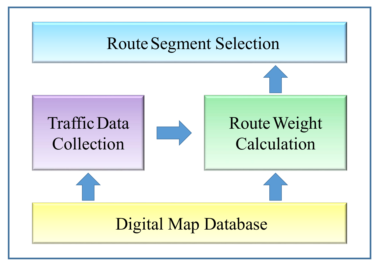
Figure 2.
The testing vehicle: PHEV vehicle (left) and gasoline vehicle (right).

Figure 3.
Travel routes in the comparison study. S: start; D: destination.
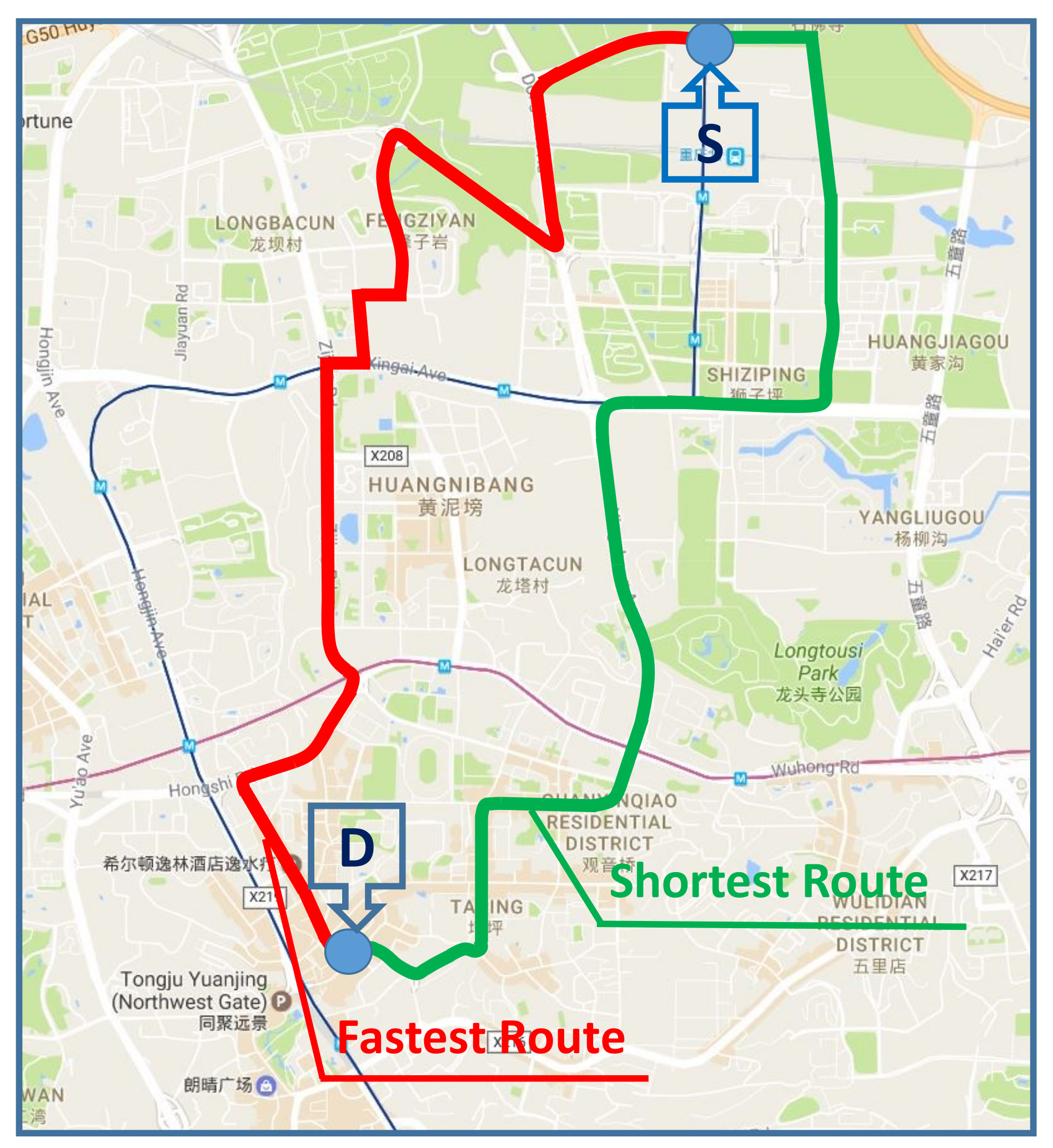
Figure 4.
Energy consumption data logging tools: OBD tool (left) and power analyzer (right).
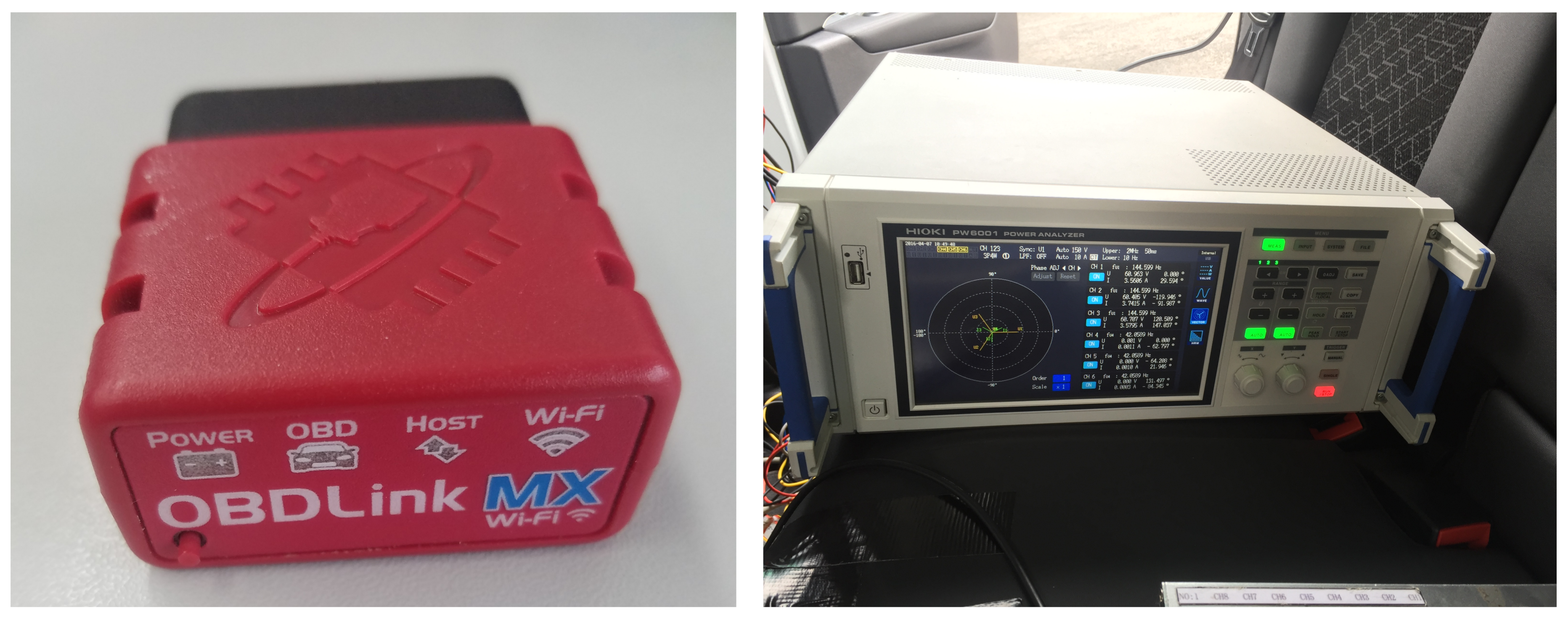
Figure 5.
Process of traffic data collection. ITS; intelligent transport system.
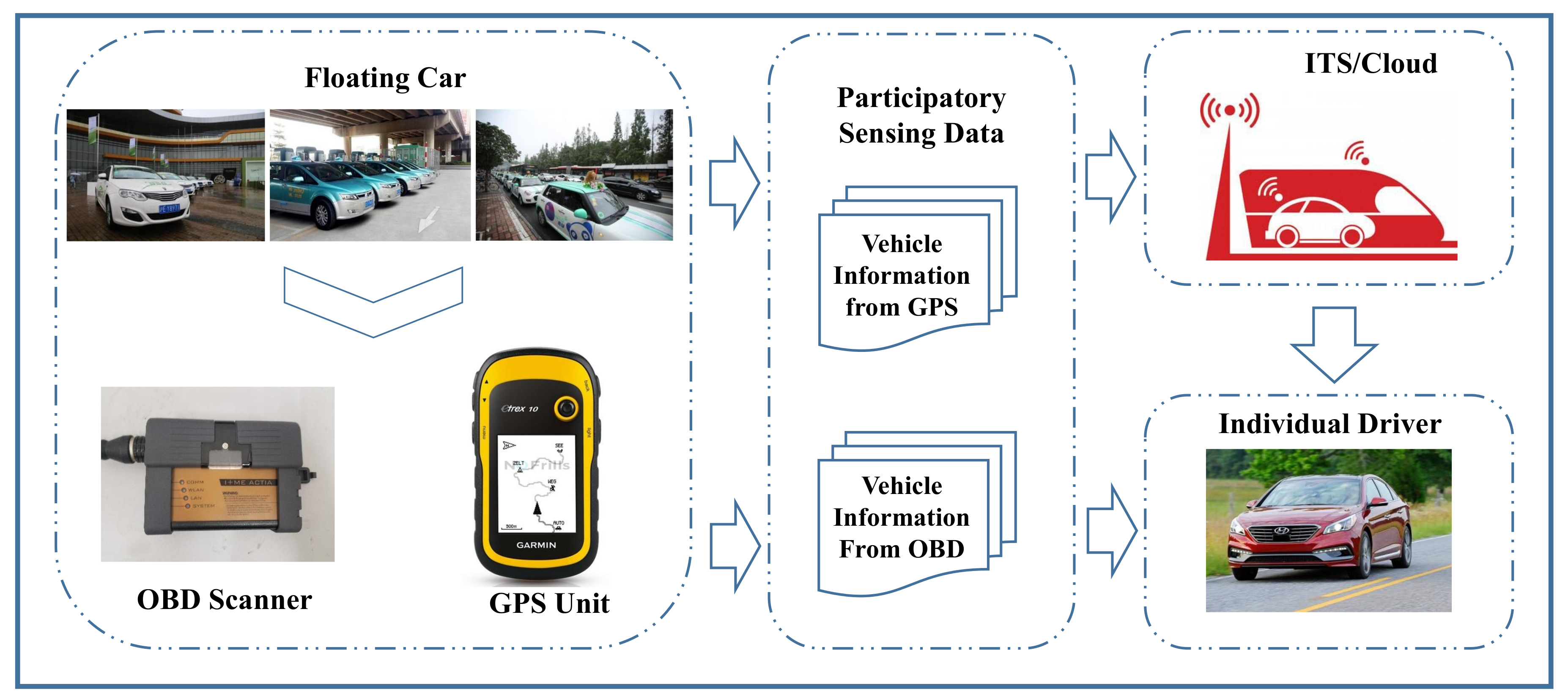
Figure 6.
Illustration of the three steps.
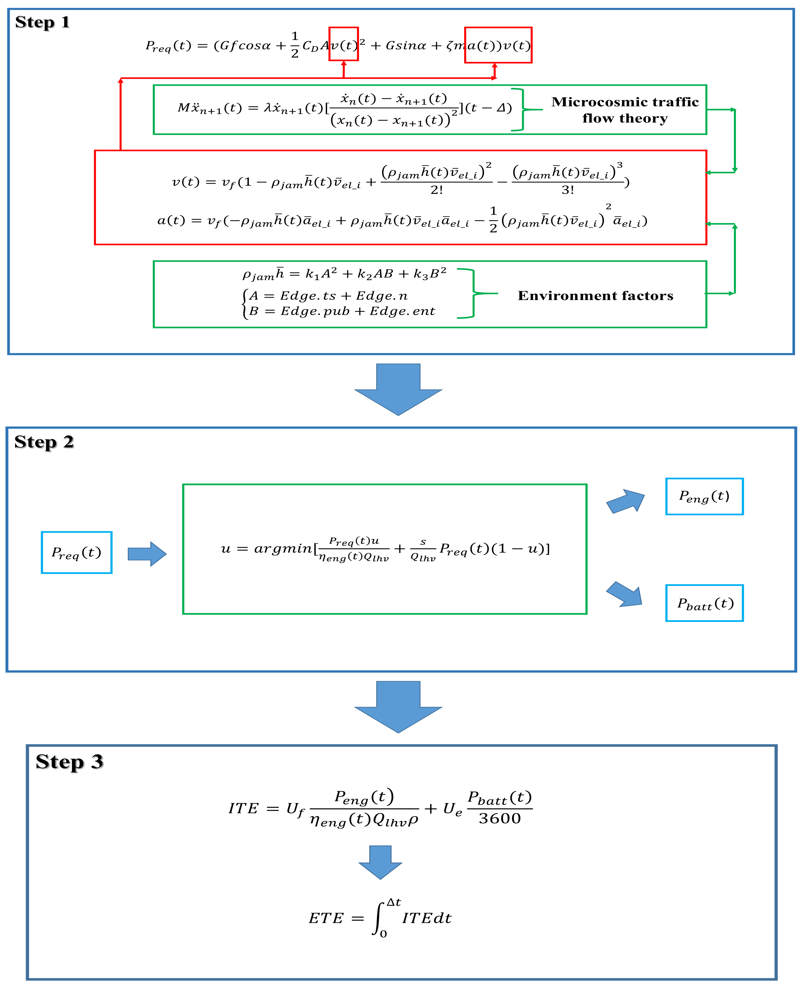
Figure 7.
Engine operating points from the benchmark test (left) and the simulation (right).

Figure 8.
Motor operation points from the benchmark test (left) and the simulation (right).
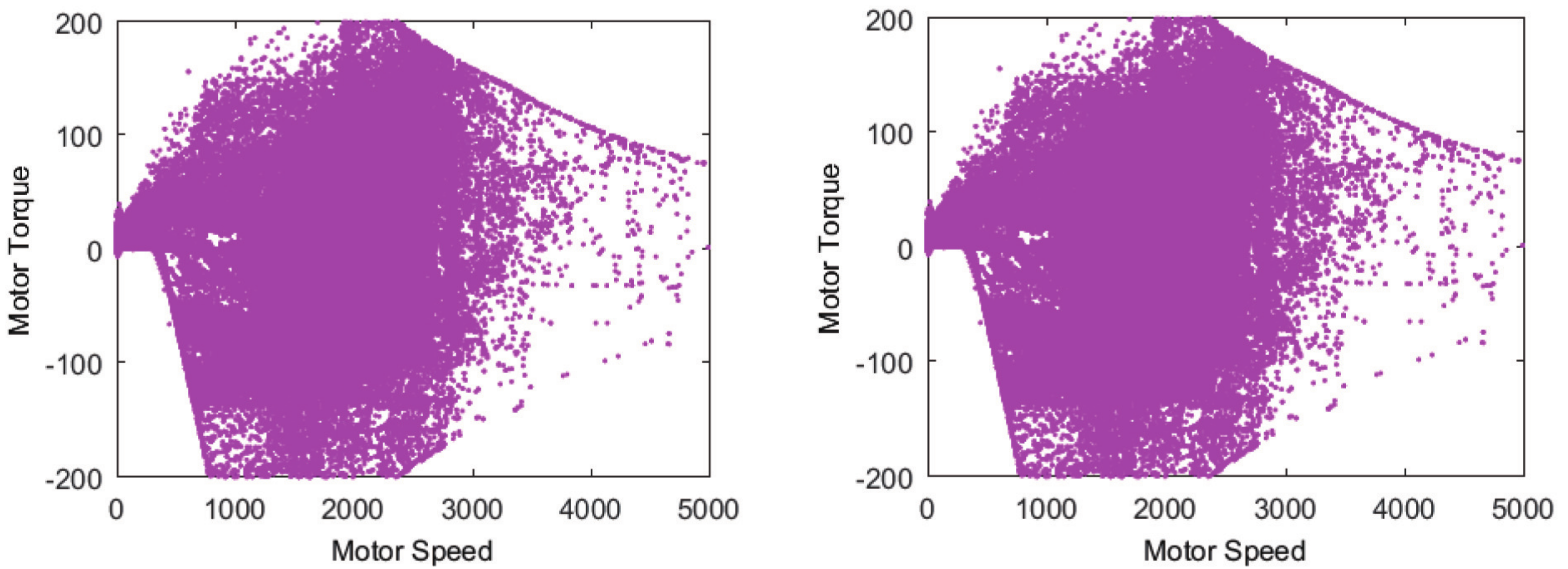
Figure 9.
Comparison of the battery SOC change in the simulation and the benchmark test.

Figure 10.
TEEM performance with various route lengths and initial battery SOCs.

Figure 11.
TEEM performance with different initial battery SOCs when the route length is 10 km.
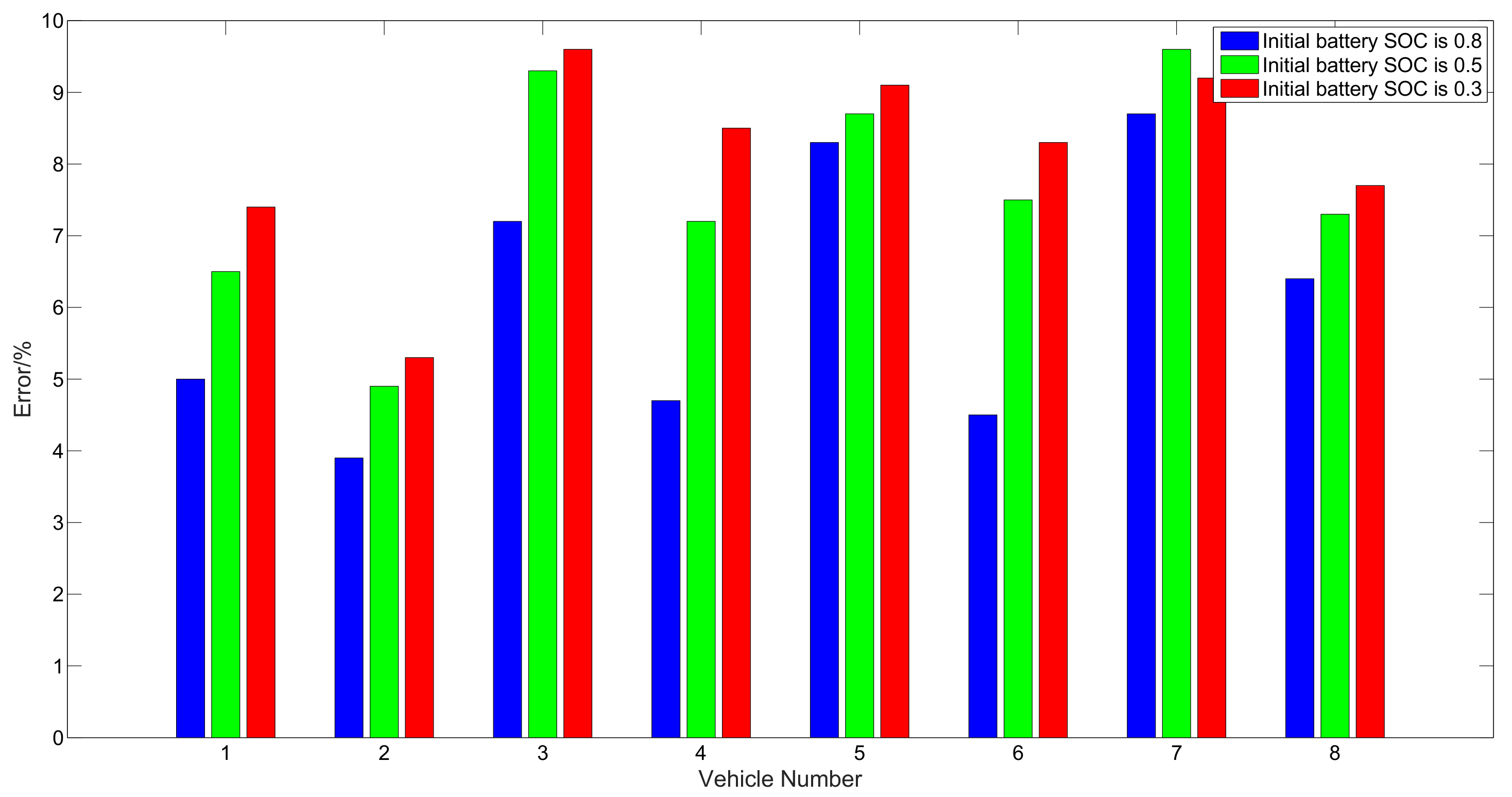
Figure 12.
TEEM performance compared with the real routes test.

Figure 13.
Illustration of the chosen routes when the initial battery SOC is 0.3.

Figure 14.
Illustration of the chosen routes when the initial battery SOC is 0.8.


Table 1.
Energy consumption of the PHEV.
| Initial Battery SOC | Route | Fuel Consumption/L | Electricity Consumption/kWh | Travel Expense/Yuan |
|---|---|---|---|---|
| 0.3 | Fastest Route (8.9 km) | 0.32 | 0.20 | 2.44 |
| Shortest Route (7.7 km) | 0.37 | 0.13 | 2.64 | |
| 0.8 | Fastest Route (8.9 km) | 0 | 0.76 | 1.36 |
| Shortest Route (7.7 km) | 0 | 0.67 | 1.20 |
Table 2.
Energy consumption of the gasoline vehicle.
| Route | Fuel Consumption/L | Travel Expense/Yuan |
|---|---|---|
| Fastest Route (8.9 km) | 0.7697 | 5.03 |
| Shortest Route (7.7 km) | 0.6514 | 4.26 |
Table 3.
The basic information of the 8 PHEVs.
| No. | Vehicle Brand | Vehicle Model |
|---|---|---|
| 1 | Hyundai | Sonata |
| 2 | Audi | A3 e-tron |
| 3 | Benz | C350el |
| 4 | Kia | Optimal |
| 5 | FAW | Hongqi H7 |
| 6 | VW | Golf GTE |
| 7 | Volvo | S60 L |
| 8 | FAW | Benteng B50 |
Table 4.
The comparison result of the two velocity sequences.
| Vehicle Velocity Difference (m/s) | The Percentage of the Total Number |
|---|---|
| ≤1 | 93.5% |
| ≤2 | 98.1% |
| ≤3 | 99.3% |
| ≤4 | 99.9% |
Table 5.
The energy consumption and travel expense when the initial battery SOC is 0.3.
| Routes | Recommended (Fastest) Route (4.8 km) | Shortest Route (4.5 km) | Optional Route (5.4 km) | |
|---|---|---|---|---|
| Items | ||||
| Fuel Consumption/L | 0.18 | 0.22 | 0.26 | |
| Electricity Consumption/kWh | 0.15 | 0.08 | 0.12 | |
| Travel Expense/Yuan | 1.43 | 1.57 | 1.91 | |
Table 6.
The energy consumption and travel expense when the initial battery SOC is 0.8.
| Routes | Fastest Route (4.8 km) | Recommended (Shortest) Route (4.5 km) | Optional Route (5.4 km) | |
|---|---|---|---|---|
| Items | ||||
| Fuel Consumption/L | 0 | 0 | 0 | |
| Electricity Consumption/kWh | 0.41 | 0.39 | 0.48 | |
| Travel Expense/Yuan | 0.74 | 0.69 | 0.86 | |
© 2017 by the authors. Licensee MDPI, Basel, Switzerland. This article is an open access article distributed under the terms and conditions of the Creative Commons Attribution (CC BY) license (http://creativecommons.org/licenses/by/4.0/).
Share and Cite
MDPI and ACS Style
Zhang, Y.; Chu, L.; Fu, Z.; Xu, N.; Guo, C.; Li, Y.; Chen, Z.; Sun, H.; Bai, Q.; Ou, Y. An Economical Route Planning Method for Plug-In Hybrid Electric Vehicle in Real World. Energies 2017, 10, 1775. https://doi.org/10.3390/en10111775
AMA Style
Zhang Y, Chu L, Fu Z, Xu N, Guo C, Li Y, Chen Z, Sun H, Bai Q, Ou Y. An Economical Route Planning Method for Plug-In Hybrid Electric Vehicle in Real World. Energies. 2017; 10(11):1775. https://doi.org/10.3390/en10111775
Chicago/Turabian StyleZhang, Yuanjian, Liang Chu, Zicheng Fu, Nan Xu, Chong Guo, Yukuan Li, Zhouhuan Chen, Hanwen Sun, Qin Bai, and Yang Ou. 2017. "An Economical Route Planning Method for Plug-In Hybrid Electric Vehicle in Real World" Energies 10, no. 11: 1775. https://doi.org/10.3390/en10111775
Note that from the first issue of 2016, this journal uses article numbers instead of page numbers. See further details here.