A Flexible Experimental Laboratory for Distributed Generation Networks Based on Power Inverters

 , , and
Abstract
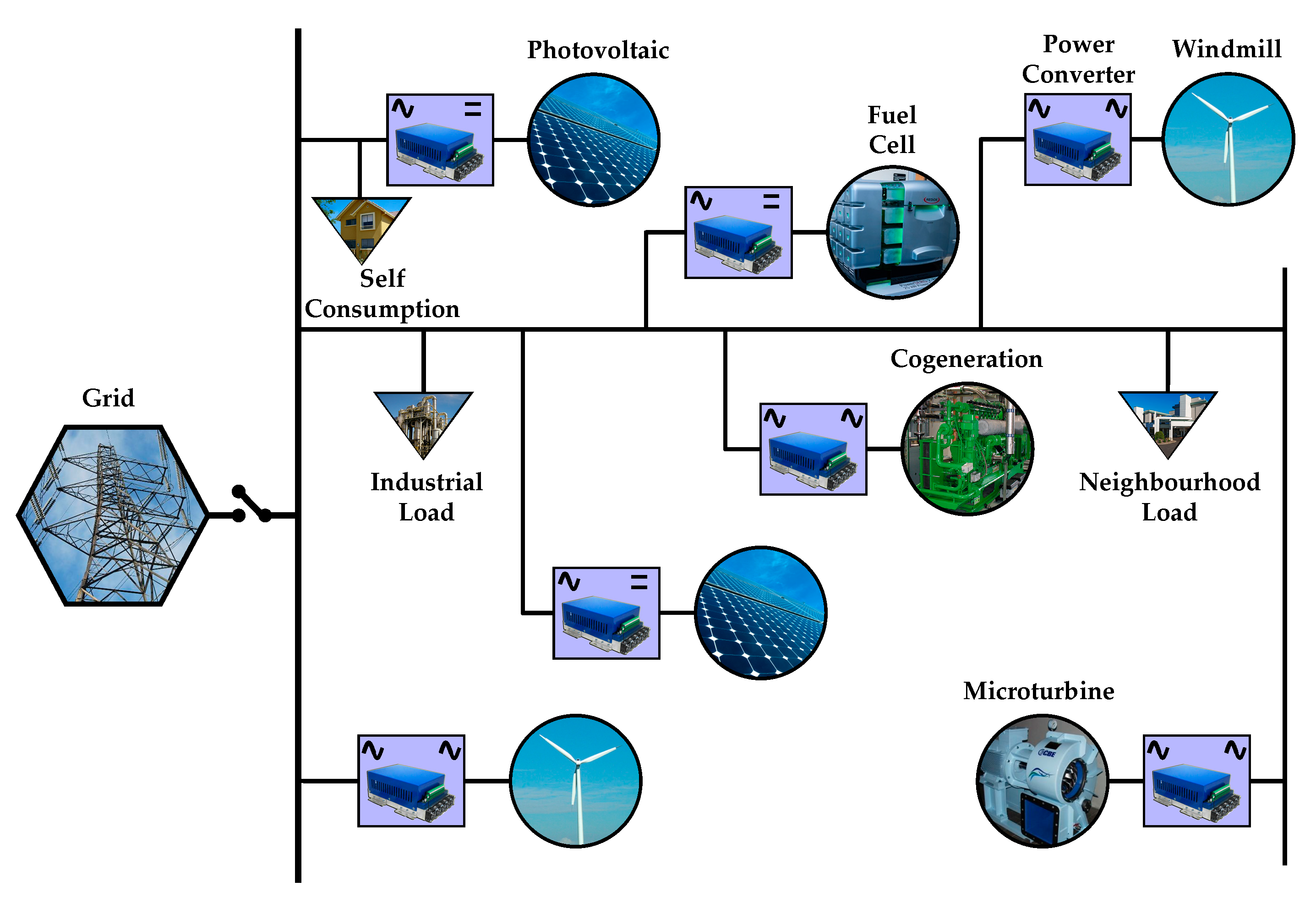
:1. Introduction
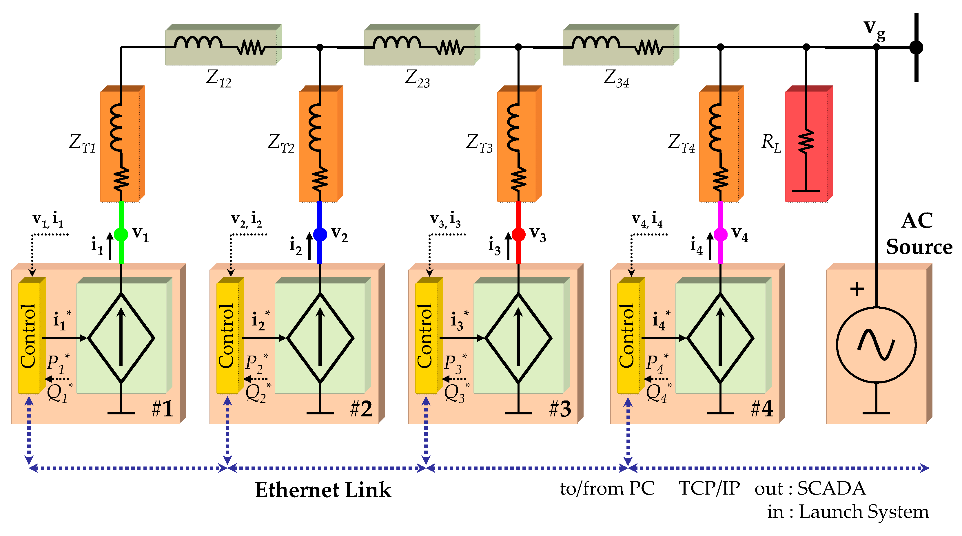
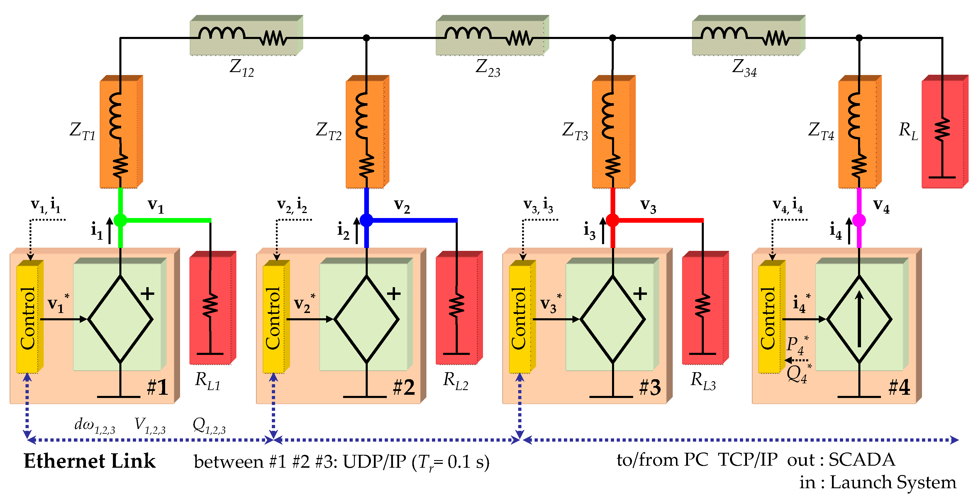
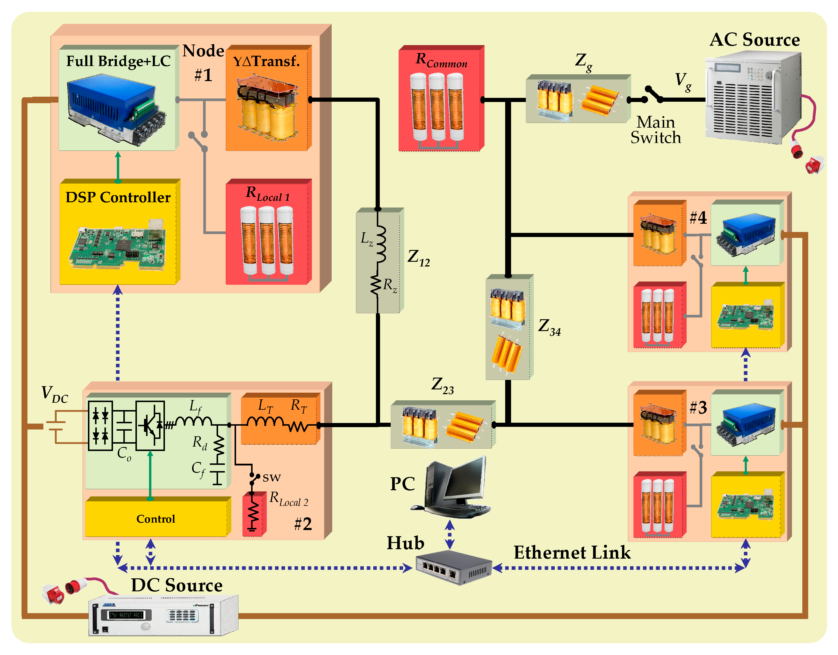
2. Experimental Network Implementation
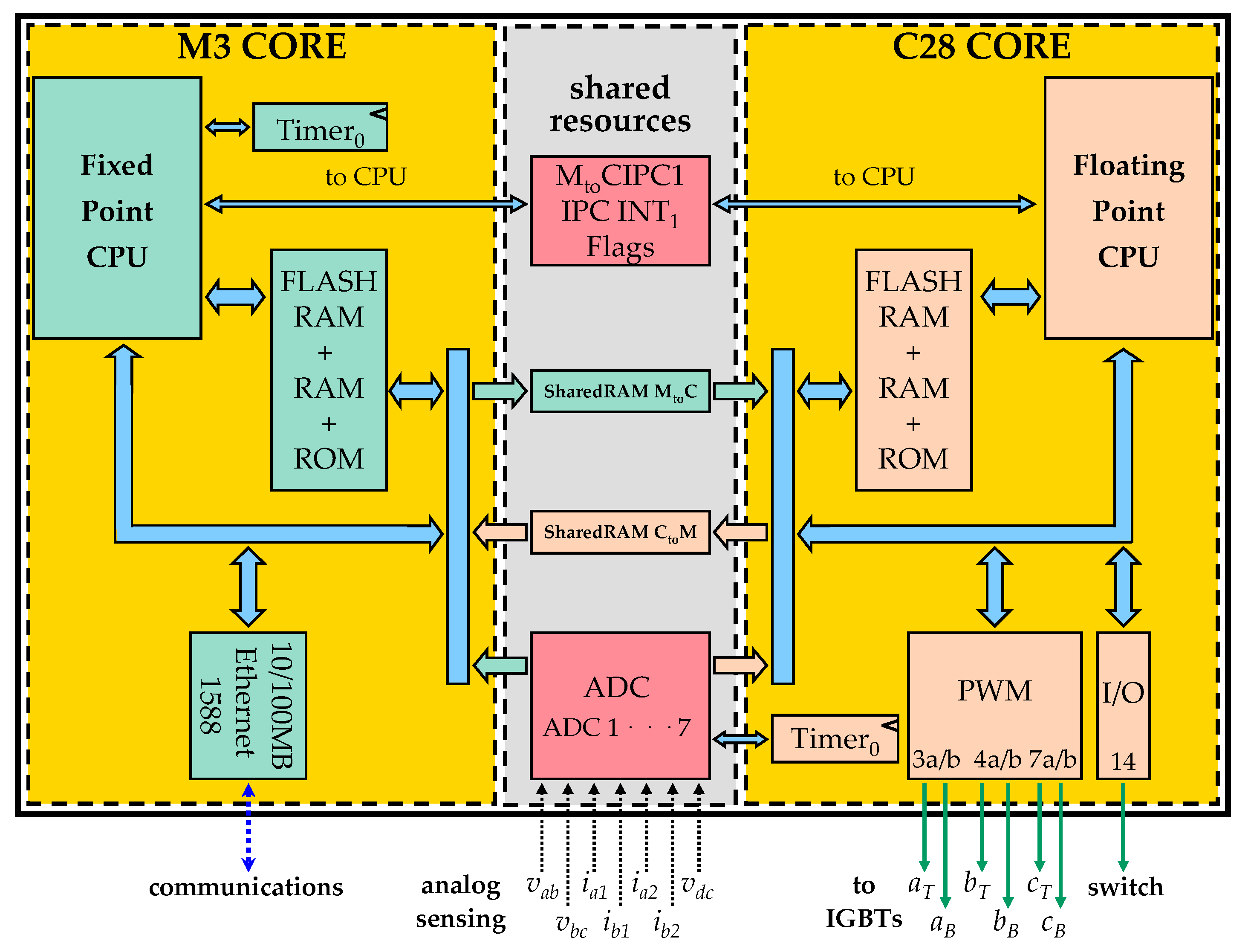
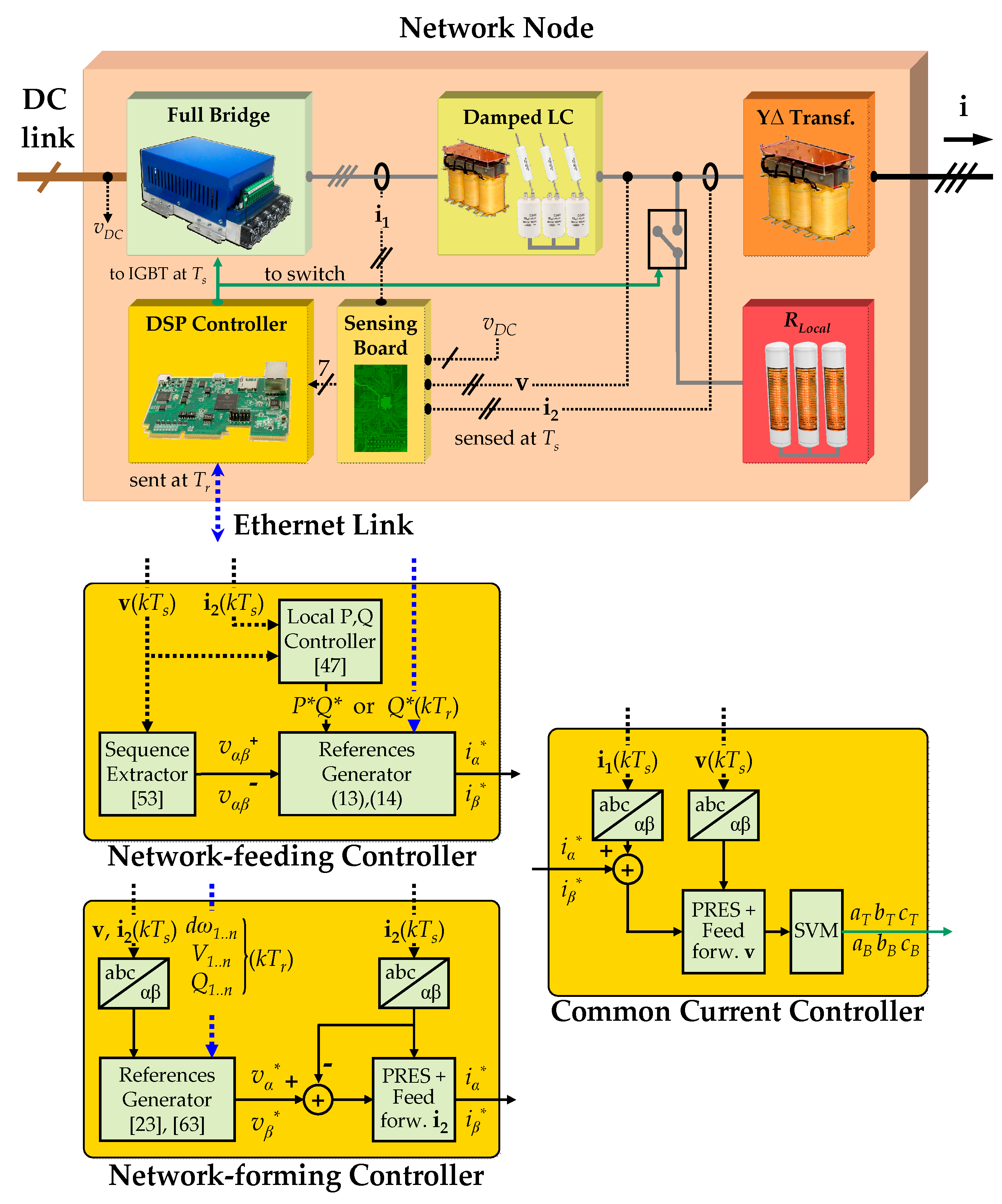
2.1. Control Platform
2.2. Power Stack
2.3. Output Filter
3. Control
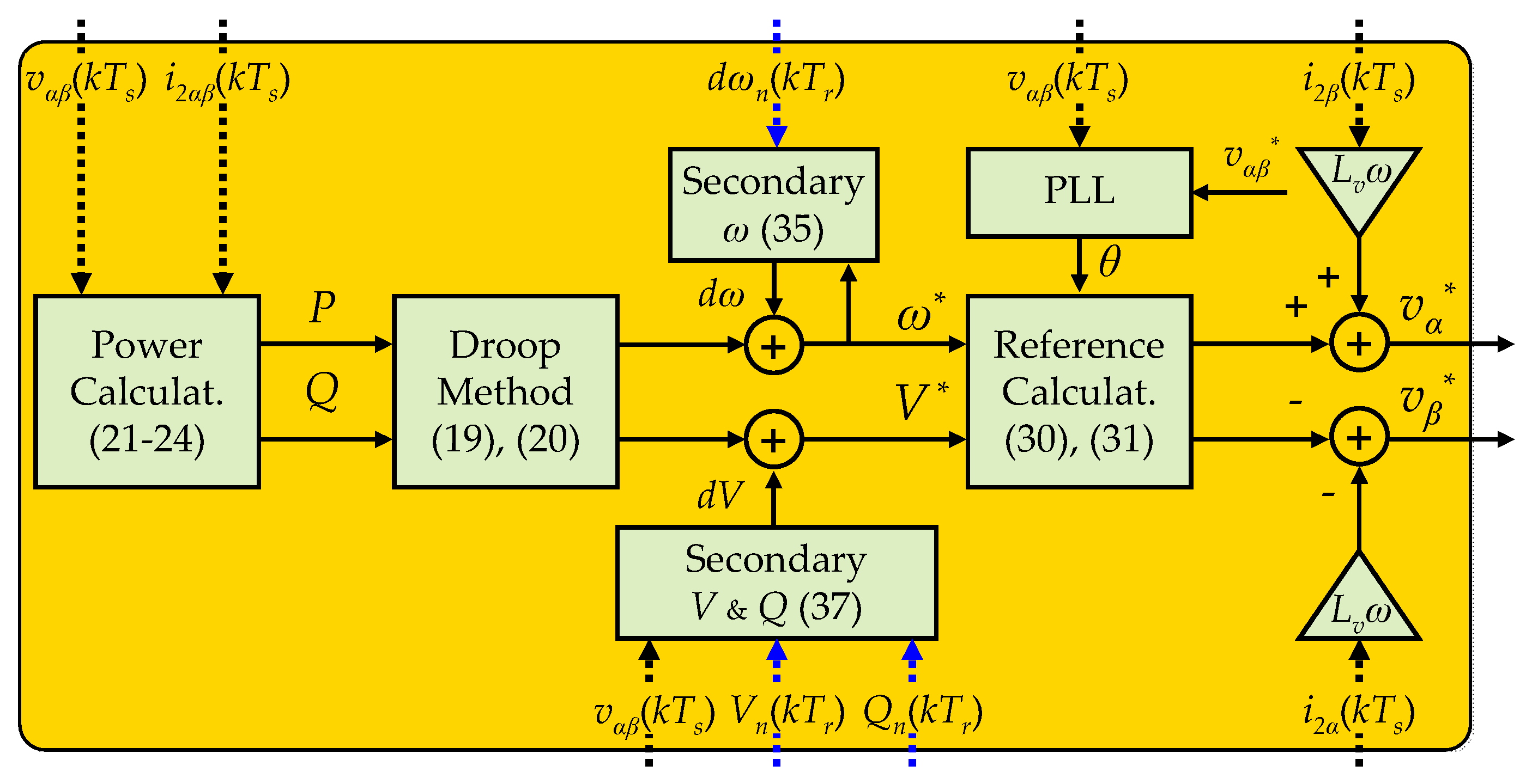
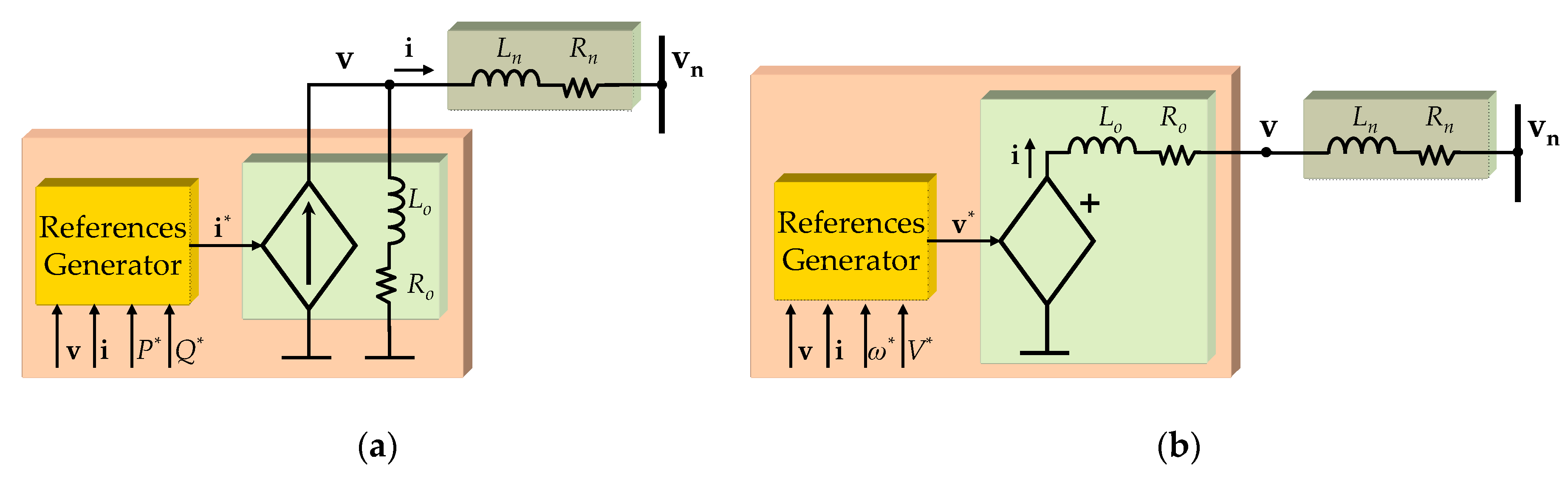
3.1. Network-Feeding Controller
3.2. Network-Forming Controller
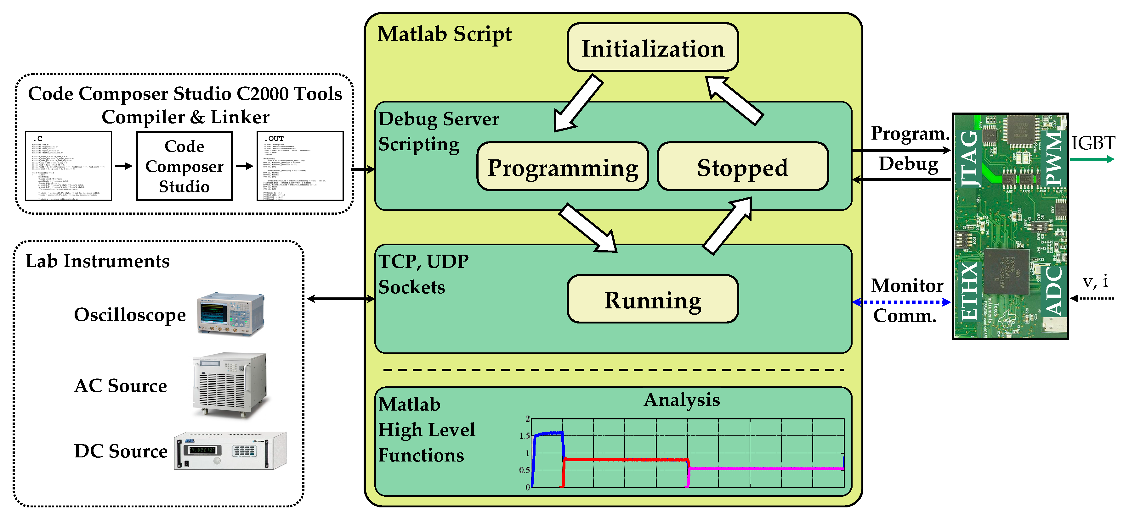
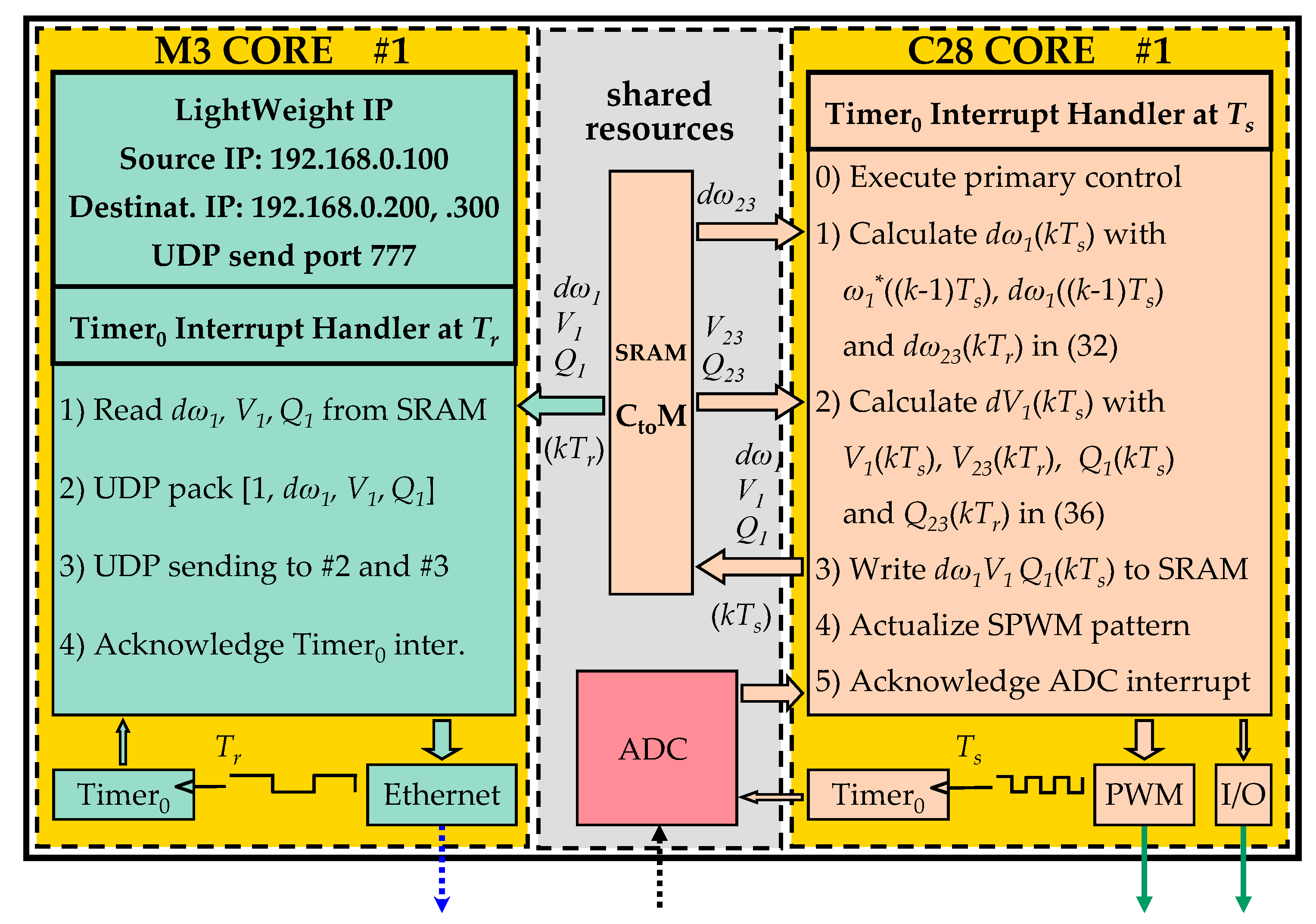
4. Communications
5. Debugging
6. Experimental Results
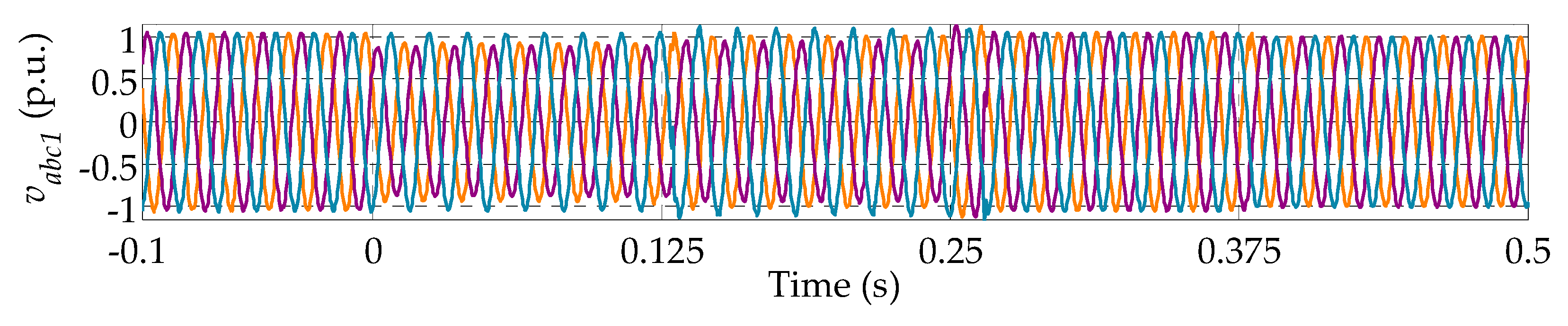
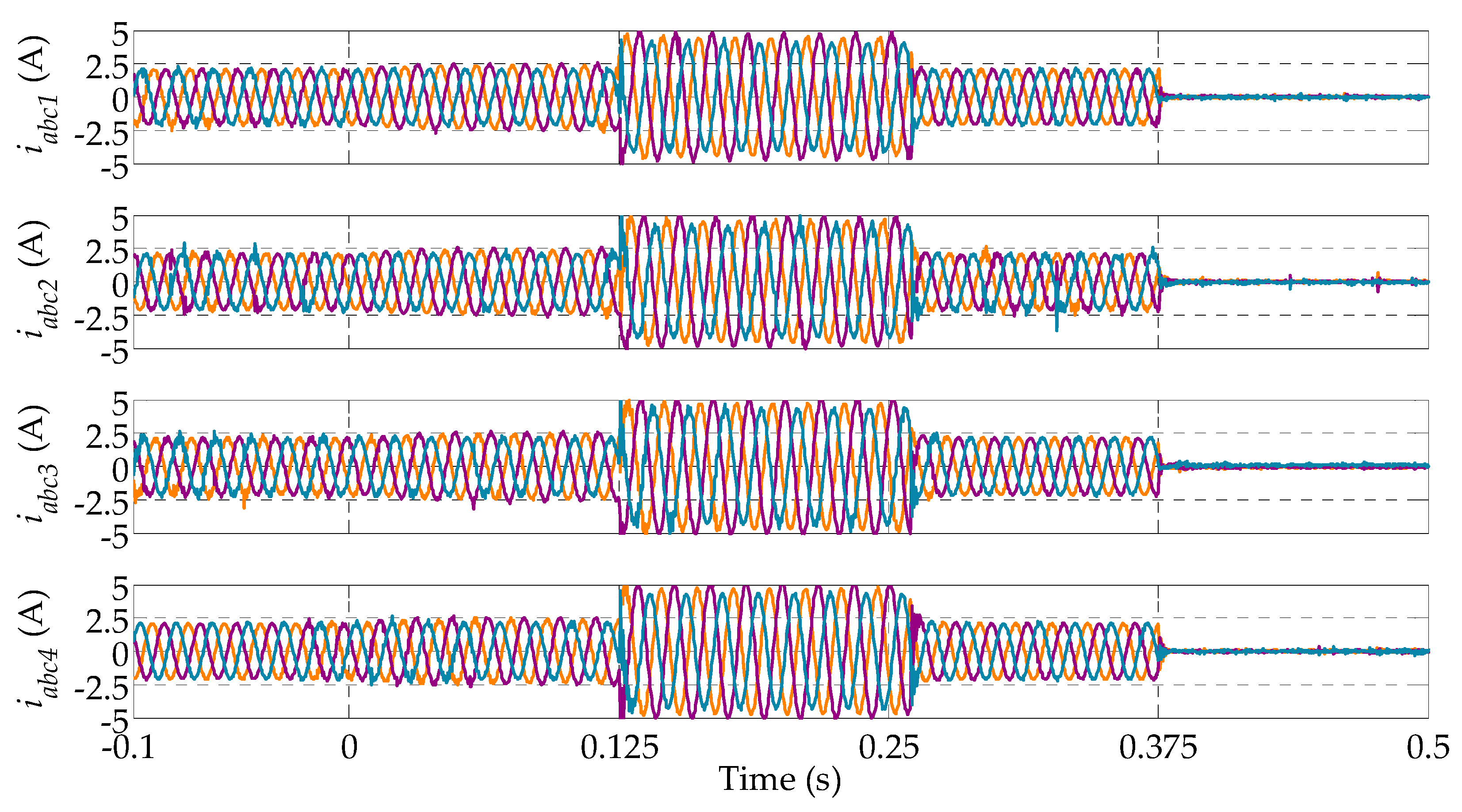
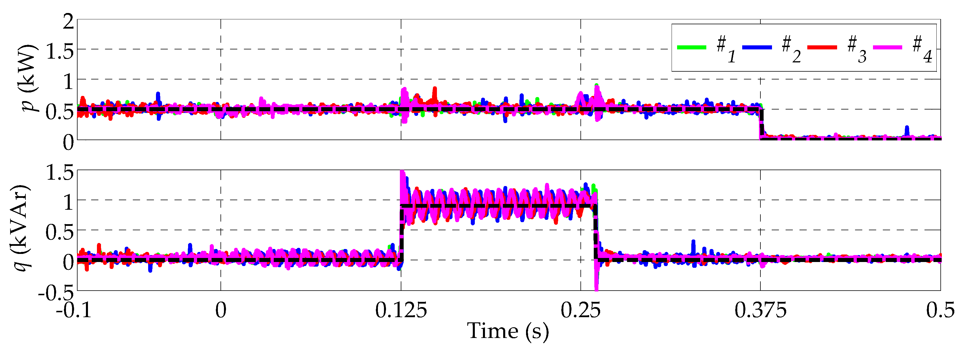
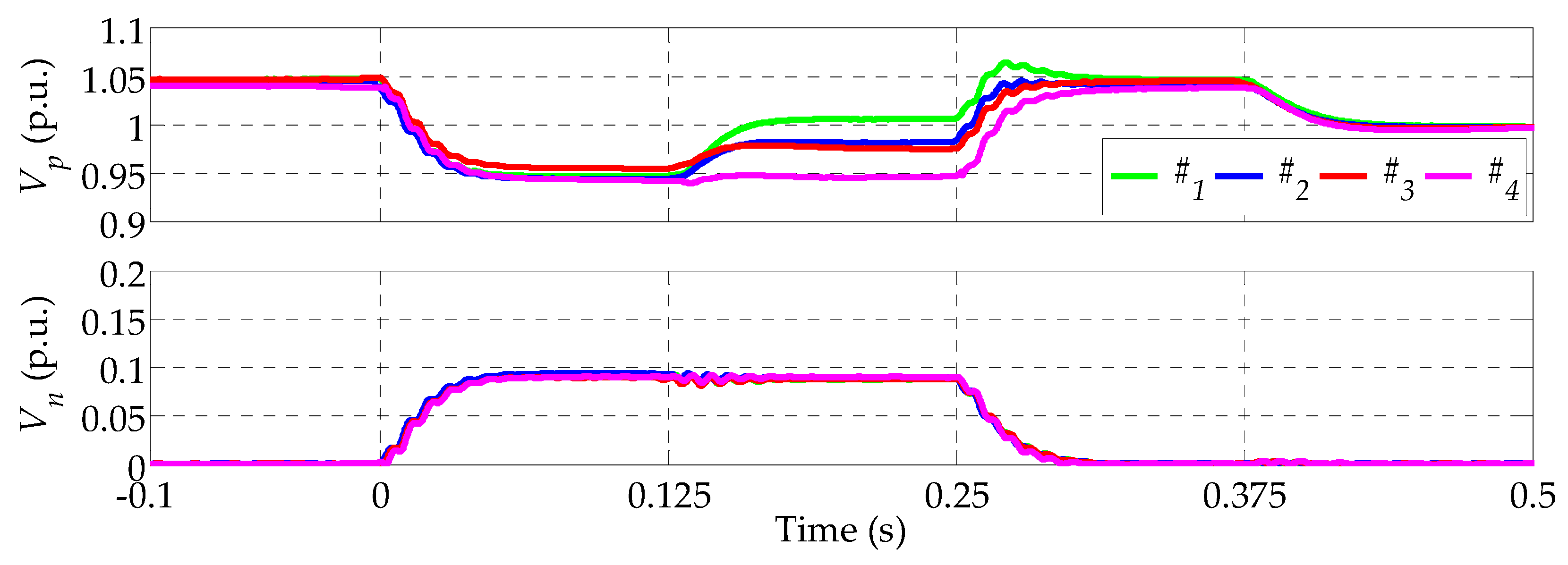
6.1. Test 1, Grid Connected Network under Voltage Sags
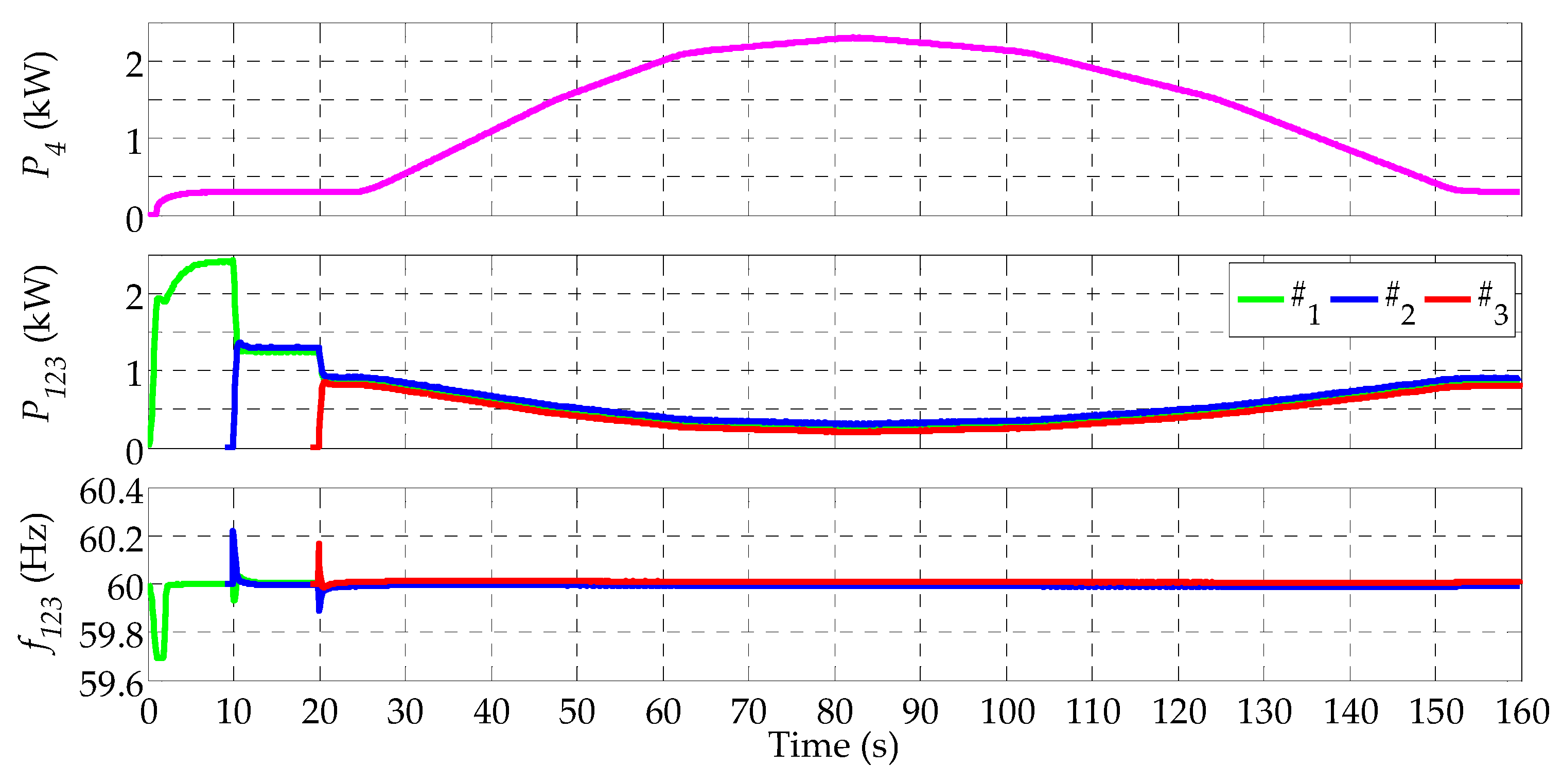
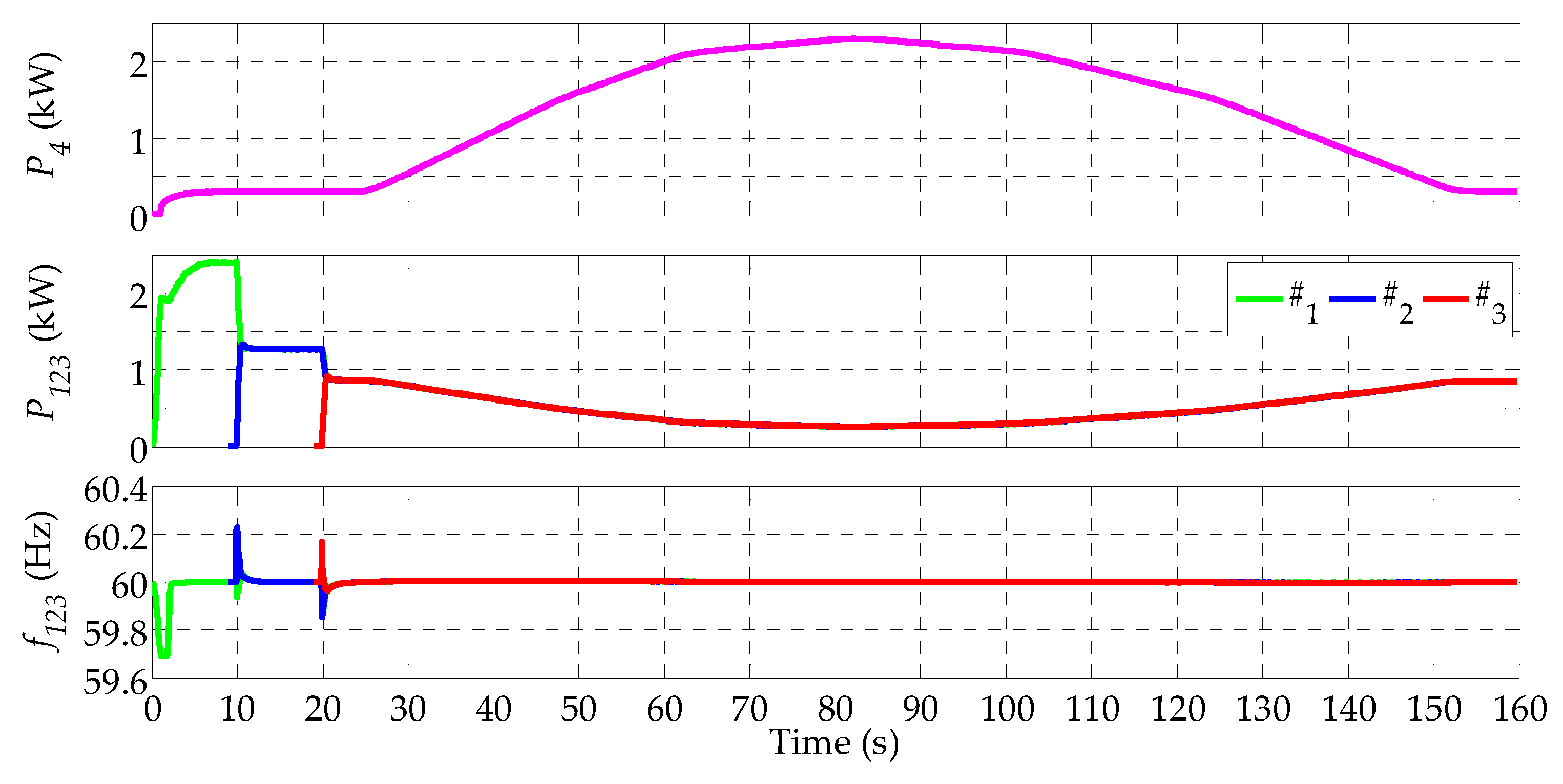
6.2. Test 2a, Islanded Microgrid with Ideal Synchronization
6.3. Test 2b, Islanded Microgrid with Clock Drift in the DSP Controllers
7. Conclusions
Acknowledgments
Author Contributions
Conflicts of Interest
References
- Adefarati, T.; Bansal, R.C. Integration of renewable distributed generators into the distribution system: A review. IET Renew. Power Gener. 2016, 10, 873–884. [Google Scholar] [CrossRef]
- Ma, Z.; Callaway, D.; Hiskens, I.A. Decentralized charging control of large populations of plug-in electric vehicles. IEEE Trans. Control Syst. Technol. 2013, 21, 67–78. [Google Scholar] [CrossRef]
- Kundu, S.; Hiskens, I.A. Overvoltages due to synchronous tripping of plug-in electric-vehicle chargers following voltage dips. IEEE Trans. Power Del. 2014, 29, 1147–1156. [Google Scholar] [CrossRef]
- IEEE Standards Association. IEEE Application Guide for IEEE Std 1547, IEEE Standard for Interconnecting Distributed Resources with Electric Power Systems; IEEE Std. 1547.2-2008; IEEE Standards Association: Piscataway, NJ, USA, 2009. [Google Scholar]
- Altin, M.; Goksu, O.; Teodorescu, R.; Rodriguez, P.; Jensen, B.-B.; Helle, L. Overview of recent grid codes for wind power integration. In Proceedings of the 12th International Conference on Optimization of Electrical and Electronic Equipment, Brasov, Romania, 20–22 May 2010; pp. 1152–1160. [Google Scholar]
- Troester, E. New German grid codes for connecting PV systems to the medium voltage power grid. In Proceedings of the 2nd International Workshop Concentrating Photovoltaic Power Plants, Darmstadt, Germany, 9–10 March 2009; pp. 1–4. [Google Scholar]
- Rocabert, J.; Azevedo, G.M.S.; Luna, A.; Guerrero, J.M.; Candela, J.I.; Rodríguez, P. Intelligent connection agent for three-phase grid-connected microgrids. IEEE Trans. Power Electron. 2011, 26, 2993–3005. [Google Scholar] [CrossRef]
- Rocabert, J.; Luna, A.; Blaabjerg, F.; Rodríguez, P. Control of power converters in AC microgrids. IEEE Trans. Power Electron. 2012, 27, 4734–4749. [Google Scholar] [CrossRef]
- Bollen, M.H.J. Understanding Power Quality Problems: Voltage Sags and Interruptions, 1st ed.; IEEE Press: New York, NY, USA, 2000. [Google Scholar]
- Milicua, A.; Abad, G.; Rodriguez Vidal, M.A. Online reference limitation method of shunt-connected converters to the grid to avoid exceeding voltage and current limits under unbalanced operation—Part I: Theory. IEEE Trans. Energy Convers. 2015, 30, 852–863. [Google Scholar] [CrossRef]
- Guo, X.; Zhang, X.; Wang, B.; Wu, W.; Guerrero, J.M. Asymmetrical grid fault ride-through strategy of three-phase grid-connected inverter considering network impedance impact in low-voltage grid. IEEE Trans. Power Electron. 2014, 29, 1064–1068. [Google Scholar] [CrossRef]
- Tsili, M.; Papathanassiou, S. A review of grid code technical requirements for wind farms. IET Renew. Power Gen. 2009, 3, 308–332. [Google Scholar] [CrossRef]
- Camacho, A.; Castilla, M.; Miret, J.; Borrell, A.; Garcia de Vicuña, L. Active and reactive power strategies with peak current limitation for distributed generation inverters during unbalanced grid faults. IEEE Trans. Ind. Electron. 2015, 62, 1515–1525. [Google Scholar] [CrossRef]
- Miret, J.; Camacho, A.; Castilla, M.; García de Vicuña, J.L.; de la Hoz, J. Reactive current injection protocol for low-power rating distributed generation sources under voltage sags. IET Power Electron. 2015, 8, 879–886. [Google Scholar] [CrossRef] [Green Version]
- Guerrero, J.M.; Chandorkar, M.; Lee, T.-L.; Loh, P.C. Advanced control architectures for intelligent microgrids—Part I: Decentralized and hierarchical control. IEEE Trans. Ind. Electron. 2013, 60, 1254–1262. [Google Scholar] [CrossRef]
- Guerrero, J.M.; Loh, P.C.; Lee, T.-L.; Chandorkar, M. Advanced control architectures for intelligent microgrids—Part II: Power quality, energy storage, and AC/DC microgrids. IEEE Trans. Ind. Electron. 2013, 60, 1263–1270. [Google Scholar] [CrossRef]
- Lasseter, R.; Piagi, P. MicroGrids: A conceptual solution. In Proceedings of the IEEE 35th Power Electronics Specialists Conference, Aachen, Germany, 20–25 June 2004; pp. 4285–4290. [Google Scholar]
- Tuladhar, A.; Jin, H.; Unger, T.; Mauch, K. Control of parallel inverters in distributed AC power systems with consideration offline impedance. IEEE Trans. Ind. Appl. 2000, 36, 321–328. [Google Scholar] [CrossRef]
- Lopes, J.A.P.; Moreira, C.L.; Madureira, A.G. Defining control strategies for microgrids islanded operation. IEEE Trans. Power Systems. 2006, 21, 916–924. [Google Scholar] [CrossRef]
- Nasirian, V.; Shafiee, Q.; Guerrero, J.M.; Lewis, F.L.; Davoudi, A. Droop-free distributed control for AC microgrids. IEEE Trans. Power Electron. 2016, 31, 1600–1617. [Google Scholar] [CrossRef]
- Liu, W.; Gu, W.; Sheng, W.; Meng, X.; Wu, Z.; Chen, W. Decentralized multi-agent system-based cooperative frequency control for autonomous microgrids with communication constraints. IEEE Trans. Sustain. Energy 2014, 5, 446–456. [Google Scholar] [CrossRef]
- Guo, F.; Wen, C.; Mao, J.; Song, Y.-D. Distributed secondary voltage and frequency restoration control of droop-controlled inverter-based microgrids. IEEE Trans. Ind. Electron. 2015, 62, 4355–4364. [Google Scholar] [CrossRef]
- Lu, L.Y.; Chu, C.C. Consensus-based droop control synthesis for multiple DICs in isolated micro-grids. IEEE Trans. Power Syst. 2015, 30, 2243–2256. [Google Scholar] [CrossRef]
- Xin, H.; Zhao, R.; Zhang, L.; Wang, Z.; Wong, K.P.; Wei, W. A decentralized hierarchical control structure and self-optimizing control strategy for F-P type DGs in islanded microgrids. IEEE Trans. Smart Grid. 2016, 7, 3–5. [Google Scholar] [CrossRef]
- Hua, M.; Hu, H.; Xing, Y.; Guerrero, J.M. Multilayer control for inverters in parallel operation without intercommunications. IEEE Trans. Power Electron. 2012, 27, 3651–3663. [Google Scholar] [CrossRef]
- Rey, J.M.; Marti, P.; Velasco, M.; Miret, J.; Castilla, M. Secondary Switched Control with no Communications for Islanded Microgrids. IEEE Trans. Ind. Electron. 2017, in press. [Google Scholar] [CrossRef]
- Lidula, N.; Rajapakse, A. Microgrids research: A review of experimental microgrids and test systems. Renew. Sustain. Energy Rev. 2011, 15, 186–202. [Google Scholar] [CrossRef]
- Lasseter, R.H.; Eto, J.H.; Schenkman, B.; Stevens, J.; Vollkommer, H.; Klapp, D.; Linton, E.; Hurtado, H.; Roy, J. CERTS microgrid laboratorytest bed. IEEE Trans. Power Del. 2011, 26, 325–332. [Google Scholar] [CrossRef]
- Salehi, V.; Mohamed, A.; Mazloomzadeh, A.; Mohammed, O.A. Laboratory-based smart power system, Part I: Design and system development. IEEE Trans. Smart Grid. 2012, 3, 1394–1404. [Google Scholar] [CrossRef]
- Salehi, V.; Mohamed, A.; Mazloomzadeh, A.; Mohammed, O.A. Laboratory-based smart power system, Part II: Control, monitoring, and protection. IEEE Trans. Smart Grid. 2012, 3, 1405–1417. [Google Scholar] [CrossRef]
- Rasheduzzaman, M.; Chowdhury, B.H.; Bhaskara, S. Converting an old machines lab into a functioning power network with a microgrid for education. IEEE Trans. Power Syst. 2014, 29, 1952–1962. [Google Scholar] [CrossRef]
- Meng, L.; Luna, A.; Rodríguez Díaz, E.; Sun, B.; Dragicevic, T.; Savaghebi, M.; Vasquez, J.C.; Guerrero, J.M.; Graells, M.; Andrade, F. Flexible system integration and advanced hierarchical control architectures in the microgrid research laboratory of Aalborg University. IEEE Trans. Ind. Appl. 2016, 52, 1736–1749. [Google Scholar] [CrossRef]
- Buccella, C.; Cecati, C.; Latafat, H. Digital control of power converters—A survey. IEEE Trans. Industr. Inform. 2012, 8, 437–447. [Google Scholar] [CrossRef]
- Pacific Power Source. Available online: https://pacificpower.com/Resources/Documents/360AMX_Datasheet.pdf (accessed on 10 July 2017).
- American Reliance. Available online: http://www.programmablepower.com/products (accessed on 10 July 2017).
- Bueno, E.J.; Hernandez, A.; Rodriguez, F.J.; Giron, C.; Mateos, R.; Cobreces, S. A DSP- and FPGA-based industrial control with high-speed communication interfaces for grid converters applied to distributed power generation systems. IEEE Trans. Ind. Electron. 2009, 56, 654–669. [Google Scholar] [CrossRef]
- Lu, X.; Guerrero, J.M.; Sun, K.; Vasquez, J.C.; Teodorescu, R.; Huang, L. Hierarchical Control of Parallel AC-DC Converter Interfaces for Hybrid Microgrids. IEEE Trans. Smart Grid. 2014, 5, 683–692. [Google Scholar] [CrossRef]
- Mandal, K.; Banerjee, S. Synchronization phenomena in microgrids with capacitive coupling. IEEE Trans. Emerg. Sel. Top. Circuits Syst. 2015, 5, 364–371. [Google Scholar] [CrossRef]
- Velasco, M.; Marti, P.; Camacho, A.; Miret, J.; Castilla, M. Synchronization of local integral controllers for frequency restoration in islanded microgrids. In Proceedings of the 42nd Annual Conference of the IEEE Industrial Electronics Society, Firenze, Italy, 24–27 October 2016. [Google Scholar]
- Schiffer, J.; Ortega, R.; Hans, C.A.; Raisch, J. Droop-controlled inverter-based microgrids are robust to clock drifts. In Proceedings of the 2015 American Control Conference, Chicago, IL, USA, 1–3 July 2015; pp. 2341–2346. [Google Scholar]
- Schiffer, J.; Hans, C.A.; Kral, T.; Ortega, R.; Raisch, J. Modelling, analysis and experimental validation of clock drift effects in low-inertia power systems. IEEE Trans. Ind. Electron. 2016, 64, 5942–5951. [Google Scholar] [CrossRef]
- Torres-Martínez, J.; Castilla, M.; Miret, J.; Rey, J.M.; Moradi-Ghahderijani, M. Experimental study of clock drift impact over droop-free distributed control for industrial microgrids. In Proceedings of the 42nd Annual Conference of the IEEE Industrial Electronics Society, Beijing, China, 29 October–1 November 2017. [Google Scholar]
- Decotignie, J.D. Ethernet-based real-time and industrial communications. Proc. IEEE 2005, 93, 1102–1117. [Google Scholar] [CrossRef]
- Texas Instruments, F28M36x Concerto Microcontrollers Report SPRS825C. Available online: http://www.ti.com/product/F28M36P63C2 (accessed on 10 July 2017).
- Texas Instruments, H63C2 Concerto Experimenter Kit. Available online: http://www.ti.com/tool/tmdsdock28m36 (accessed on 10 July 2017).
- MTL-CBI0060F12IXHF Data Sheet. Available online: http://www.e-guasch.com (accessed on 10 July 2017).
- Figueres, E.; Garcera, G.; Sandia, J.; Gonzalez-Espin, F.; Rubio, J.C. Sensitivity study of the dynamics of three-phase photovoltaic inverters with an LCL grid filter. IEEE Trans. Ind. Electron. 2009, 56, 706–717. [Google Scholar] [CrossRef]
- Liserre, M.; Teodorescu, R.; Blaabjerg, F. Stability of photovoltaic and wind turbine grid-connected inverters for a large set of grid impedance values. IEEE Trans. Power Electron. 2006, 21, 263–272. [Google Scholar] [CrossRef]
- Liu, J.; Zhou, L.; Yu, X.; Li, B.; Zheng, C. Design and analysis of an LCL circuit-based three-phase grid-connected inverter. IET Power Electron. 2017, 10, 232–239. [Google Scholar] [CrossRef]
- Blaabjerg, F.; Teodorescu, R.; Liserre, M.; Timbus, A.V. Overview of control and grid synchronization for distributed power generation systems. IEEE Trans. Ind. Electron. 2006, 53, 1398–1409. [Google Scholar] [CrossRef]
- Zmood, D.N.; Holmes, D.G.; Bode, G.H. Frequency-domain analysis of three-phase linear current regulators. IEEE Trans. Ind. Appl. 2001, 37, 601–610. [Google Scholar] [CrossRef]
- Bollen, M.H.J. Algorithms for characterizing measured three phase unbalanced voltage dips. IEEE Trans. Power Del. 2003, 18, 937–944. [Google Scholar] [CrossRef]
- Matas, J.; Castilla, M.; Miret, J.; Garcia de Vicuña, L.; Guzman, R. An adaptive pre-filtering method to improve the speed/accuracy trade-off of voltage sequence detection methods under adverse grid conditions. IEEE Trans. Ind. Electron. 2014, 61, 2139–2151. [Google Scholar] [CrossRef]
- Sosa, J.L.; Castilla, M.; Miret, J.; Matas, J.; Al-Turki, Y.A. Control strategy to maximize the power capability of PV three-phase inverters during voltage sags. IEEE Trans. Power Electron. 2016, 31, 3314–3323. [Google Scholar] [CrossRef]
- Trujillo Rodriguez, C.; Velasco de la Fuente, D.; Garcera, G.; Figueres, E.; Guacaneme Moreno, J.A. Reconfigurable control scheme for a PV microinverter working in both grid-connected and island modes. IEEE Trans. Ind. Electron. 2013, 60, 1582–1595. [Google Scholar] [CrossRef]
- Baran, M.E.; El-Markabi, I.M. A multiagent-based dispatching scheme for distributed generators for voltage support on distribution feeders. IEEE Trans. Power Syst. 2007, 22, 52–59. [Google Scholar] [CrossRef]
- Bottura, R.; Borghetti, A. Simulation of the Volt/Var control in distribution feeders by means of a networked multiagent system. IEEE Trans. Ind. Inform. 2014, 10, 2340–2353. [Google Scholar] [CrossRef]
- Camacho, A.; Castilla, M.; Miret, J.; Matas, J.; Guzman, R.; de Sousa-Pérez, O.; Martí, P.; García de Vicuña, L. Control strategies based on effective power factor for distributed generation power plants during unbalanced grid voltage. In Proceedings of the 39th Annual Conference of the IEEE Industrial Electronics Society, Vienna, Austria, 10–13 November 2013; pp. 7134–7139. [Google Scholar]
- Miret, J.; Camacho, A.; Castilla, M.; Garcia de Vicuña, L.; Matas, J. Control scheme with voltage support capability for distributed generation inverters under voltage sags. IEEE Trans. Power Electron. 2013, 28, 5252–5262. [Google Scholar] [CrossRef]
- Rodriguez, P.; Timbus, A.V.; Teodorescu, R.; Liserre, M.; Blaabjerg, F. Flexible active power control of distributed power generation systems during grid faults. IEEE Trans. Ind. Electron. 2007, 54, 2583–2592. [Google Scholar] [CrossRef]
- Camacho, A.; Castilla, M.; Miret, J.; Vasquez, J.C.; Alarcon-Gallo, E. Flexible voltage support control for three-phase distributed generation inverters under grid fault. IEEE Trans. Ind. Electron. 2013, 60, 1429–1441. [Google Scholar] [CrossRef]
- Vasquez, J.C.; Guerrero, J.M.; Miret, J.; Castilla, M.; Garcia de Vicuña, L. Hierarchical control of intelligent microgrids. IEEE Ind. Electron. Mag. 2010, 4, 23–29. [Google Scholar] [CrossRef]
- Guerrero, J.M.; Vasquez, J.C.; Matas, J.; Garcia de Vicuña, L.; Castilla, M. Hierarchical control of droop-controlled AC and DC microgrids—A general approach towards standardization. IEEE Trans. Ind. Electron. 2011, 58, 158–172. [Google Scholar] [CrossRef]
- Li, B.; Zhou, L.; Yu, X.; Zheng, C.; Liu, J. Improved power decoupling control strategy based on virtual synchronous generator. IET Power Electronics. 2017, 10, 462–470. [Google Scholar] [CrossRef]
- Guerrero, J.M.; Garcia de Vicuna, L.; Matas, J.; Castilla, M.; Miret, J. Output impedance design of parallel-connected UPS inverters with wireless load-sharing control. IEEE Trans. Ind. Electron. 2005, 52, 1126–1135. [Google Scholar] [CrossRef]
- He, J.; Li, Y.W. Analysis, design, and implementation of virtual impedance for power electronics interfaced distributed generation. IEEE Trans. Ind. Appl. 2011, 47, 2525–2538. [Google Scholar] [CrossRef]
- Vasquez, J.C.; Guerrero, J.M.; Savaghebi, M.; Eloy-Garcia, J.; Teodorescu, R. Modeling, analysis, and design of stationary-reference-frame droop-controlled parallel three-phase voltage source inverters. IEEE Trans. Ind. Electron. 2013, 60, 1271–1280. [Google Scholar] [CrossRef]
- Katiraei, F.; Iravani, R.; Hatziargyriou, N.; Dimeas, A. Microgrids management. IEEE Power Energy Mag. 2008, 6, 54–65. [Google Scholar] [CrossRef]
- Walsh, G.C.; Ye, H. Scheduling of networked control systems. IEEE Control Systems Mag. 2001, 21, 57–65. [Google Scholar] [CrossRef]
- Lightweight IP. Available online: http://savannah.nongnu.org/projects/lwip (accessed on 10 July 2017).
- Using the Stellaris® Ethernet Controller with Lightweight IP (lwIP). Texas Instruments Application Report SPMA025C. Available online: http://www.ti.com/lit/an/spma025c/spma025c.pdf (accessed on 10 July 2017).
- Castilla, M. (Ed.) Control Circuits in Power Electronics: Practical Issues in Design and Implementation; IET Press: London, UK, 2016. [Google Scholar]
- Debug Server Scripting. Available online: http://processors.wiki.ti.com/index.php (accessed on 10 July 2017).
- Code Composer Studio (CCS) Integrated Development Environment (IDE). Available online: http://www.ti.com/tool/ccstudio (accessed on 10 July 2017).
- Texas Instruments, Schematics F28M36x Control CARD. Available online: http://www.ti.com/tool/tmdscncd28m36 (accessed on 10 July 2017).


| Component | Model | Ratings |
|---|---|---|
| AC source | Pacific Power, 360AMX(T)-UPC32 | Input: 208/240 Vac, 50–60 Hz, 3 phase Output: 0–341 Vac l–n, 16 A, 3 phase |
| DC source | Amrel, SPS800-19 | Input: 208/240 Vac, 50–60 Hz, 3 phase Output: 0–800 Vdc, 19 A |
| IGBT bridge | Guasch, MTL-CBI0060F12IXHF | Vdc_max = 750 V, Imax_per_phase = 30 Arms, fswitch = 10 kHz |
| Isolation transformer | Eremu, 21-10309WW | Dyn11, 3 × 400/3 × 400 Vac, 5 kVAr |
| DSP controller | Texas Instruments, Concerto F28M36P63C | |
| Current sensors | Talema, AC1025 | 0–25 Adc/ac |
| Voltage sensors | Lem, LV25-P | 0–400 Vdc/ac |
| Parameter Name | Acronym | Value | Units |
|---|---|---|---|
| Grid voltage (line to neutral, l–n) | Vg | 110 | Vrms |
| Grid frequency | fg | 60 | Hz |
| DC-link voltage | VDC | 350 | V |
| DC-link capacitance | Co | 1.5 | mF |
| LC filter inductances | Lf | 5 | mH |
| LC filter capacitances | Cf | 1.5 | μF |
| LC filter damping resistors | Rd | 68 | Ω |
| Transformer equivalent inductance #1, #2 | LT1,2 | 1 | mH |
| Transformer equivalent resistance #1, #2 | RT1,2 | 0.5 | Ω |
| Transformer equivalent inductance #3, #4 | LT3,4 | 0.6 | mH |
| Transformer equivalent resistance #3, #4 | RT3,4 | 1.13 | Ω |
| Line impedances | Zg, Z12, Z23, Z34 | configurable | |
| Common resistive load | RCommon | 24/48 | Ω |
| Local resistive loads | RLocal 1…4 | 48/96 | Ω |
| Parameter Name | Acronym | Value | Units |
|---|---|---|---|
| Node nominal rated power (base power) | Sb | 1.5 | kVAr |
| Node nominal rated current | Irated | 5 | A rms |
| Global load rated power | PL | 1.5 | kW |
| Local loads rated power | PL1,2,3 | 0.25 | kW |
| Droop method virtual inductance | Lv | 10 | mH |
| Droop method virtual resistance | Rv | 0 | Ω |
| Line inductance 12 | L12 | 2 | mH |
| Line resistance 12 | R12 | 65 | mΩ |
| Line inductance 23 | L23 | 0.8 | mH |
| Line resistance 23 | R23 | 110 | mΩ |
| Line inductance 34 | L34 | 0.8 | mH |
| Line resistance 34 | R34 | 110 | mΩ |
| Active power reference | Pi* | 0.5 | kW |
| Reactive power reference nominal conditions | Qi* | 0 | kVAr |
| Reactive power reference when sag occurs | Qi* | 0.9 | kVAr |
| Sequences balancing parameters | kp, kq | 0.5 | |
| Frequency droop parameter | mp | 1 | mrad/(Ws) |
| Voltage droop parameter | nq | 10 | mV/(V Ar) |
| Proportional gain PRES voltage compensator | kpv | 1 | mA/V |
| Integral gain PRES voltage compensator | kiv | 3 | A/(Vs) |
| Proportional gain PRES current compensator | kpi | 30 | A−1 |
| Integral gain PRES current compensator | kii | 800 | (As)−1 |
| Sampling and switching rate | Ts | 100 | μs |
| Transmission rate | Tr | 100 | ms |
| Parameter Name | Acronym | Value |
|---|---|---|
| Clock drift rate of digital processor 1 | d1 | 1.0000 |
| Clock drift rate of digital processor 2 | d2 | 1.0001 |
| Clock drift rate of digital processor 3 | d3 | 0.9999 |
© 2017 by the authors. Licensee MDPI, Basel, Switzerland. This article is an open access article distributed under the terms and conditions of the Creative Commons Attribution (CC BY) license (http://creativecommons.org/licenses/by/4.0/).
Share and Cite
Miret, J.; García de Vicuña, J.L.; Guzmán, R.; Camacho, A.; Moradi Ghahderijani, M. A Flexible Experimental Laboratory for Distributed Generation Networks Based on Power Inverters. Energies 2017, 10, 1589. https://doi.org/10.3390/en10101589
Miret J, García de Vicuña JL, Guzmán R, Camacho A, Moradi Ghahderijani M. A Flexible Experimental Laboratory for Distributed Generation Networks Based on Power Inverters. Energies. 2017; 10(10):1589. https://doi.org/10.3390/en10101589
Chicago/Turabian StyleMiret, Jaume, José Luís García de Vicuña, Ramón Guzmán, Antonio Camacho, and Mohammad Moradi Ghahderijani. 2017. "A Flexible Experimental Laboratory for Distributed Generation Networks Based on Power Inverters" Energies 10, no. 10: 1589. https://doi.org/10.3390/en10101589