Quadratic Hedging of Basis Risk

Abstract

This paper examines a simple basis risk model based on correlated geometric Brownian motions. We apply quadratic criteria to minimize basis risk and hedge in an optimal manner. Initially, we derive the Föllmer–Schweizer decomposition for a European claim. This allows pricing and hedging under the minimal martingale measure, corresponding to the local risk-minimizing strategy. Furthermore, since the mean-variance tradeoff process is deterministic in our setup, the minimal martingale- and variance-optimal martingale measures coincide. Consequently, the mean-variance optimal strategy is easily constructed. Simple pricing and hedging formulae for put and call options are derived in terms of the Black–Scholes formula. Due to market incompleteness, these formulae depend on the drift parameters of the processes. By making a further equilibrium assumption, we derive an approximate hedging formula, which does not require knowledge of these parameters. The hedging strategies are tested using Monte Carlo experiments, and are compared with results achieved using a utility maximization approach.

1. Introduction

When a contingent claim is written on an asset or process that is not traded, it is natural to enquire about the effectiveness of hedging with a correlated security. In this situation the market is incomplete, and the risk that arises as a result of imperfect hedging is known as basis risk. Examples include weather derivatives, real options, options on illiquid stocks and options on large baskets of stocks.

Since not all the risk can be hedged, we are dealing with a typical incomplete market situation, in which the appetite for risk must be specified (usually in terms of a utility function). A number of authors have formulated the problem of hedging basis risk in terms of the utility maximization approach (see, e.g., Davis [1,2], Henderson [3], Henderson and Hobson [4], Monoyios [5,6] and Zariphopoulou [7]). By contrast, we shall consider the application of quadratic criteria. Our approach is similar to that of Schweizer [8] (see also Duffie and Richardson [9]), where the application was hedging futures with a correlated asset. For comprehensive reviews on the theory of quadratic hedging, the reader is directed to the works of Pham [10], Schweizer [11] and McWalter [12].

We now describe the organization of this paper. To start with, in Section 2 we provide a summary of the terminology and general theory used throughout. In particular, we discuss the two quadratic approaches of local risk minimization and mean-variance hedging. Key to the construction of hedging strategies is a decomposition of the contingent claim, known as the Föllmer–Schweizer (FS) decomposition. We also briefly describe the minimal martingale measure and the variance-optimal martingale measure.

A simple basis risk model comprising two correlated geometric Brownian motions is specified in Section 3. We assume that it is not possible to trade in the process the claim is written on, but that the second process is a security available for trade. Since the general theory is developed in terms of discounted securities, we specify the discounted dynamics of the two processes.

The FS decomposition of the claim is derived in Section 4. This is achieved by expressing the non-traded process in terms of the traded security and an orthogonal process. By using a drift-adjusted representation of the non-traded process, it is possible to construct the minimal martingale measure. The Feynman–Kac theorem can then be used to express the discounted claim price as the solution of a partial differential equation (PDE) boundary-value problem.

In Section 5 we present the hedging strategies for the two quadratic approaches. The FS decomposition makes it easy to specify the locally risk-minimizing strategy, with prices determined by taking expectations under the minimal martingale measure. Furthermore, since the mean-variance tradeoff process is deterministic under our model assumptions, the minimal martingale measure and the variance-optimal martingale measure coincide. The mean-variance optimal self-financing strategy is thus easily constructed as well.

Having obtained a PDE representation of the price of the claim and its hedge parameters, in discounted terms, Section 6 does the same in non-discounted terms by employing a simple transformation of variables. Remarkably, the PDE that emerges, for both local risk minimization and mean-variance optimization, is the familiar Black–Scholes PDE, with a “dividend yield” parameter playing a risk-adjustment role. Consequently, both approaches yield classical closed-form derivative pricing formulae for European calls and puts (which is advantageous from a computational point of view). The hedge ratios for the two quadratic criteria are different, which reflects the different attitudes to risk they imply. These results are summarized in Proposition 3.

In Section 7 we briefly introduce the utility maximization approach to our problem that was proposed by Monoyios [5,6]. In the limiting case where risk is minimized, we observe that his hedging algorithm becomes the local risk-minimizing strategy.

A disadvantage of the quadratic hedging rules, as well as the approach of Monoyios, is that they rely explicitly on drift estimates for the asset price processes. In Section 8 we make an extra assumption, based on equilibrium under the capital asset pricing model (CAPM), which allows the derivation of a “naive” approximation of the local risk-minimizing strategy. The advantage of this naive strategy is that it does not require knowledge of the drift parameters.

In Section 9 we demonstrate the effectiveness of the quadratic hedging approaches numerically and compare the results with those obtained using the Monoyios scheme and the naive strategy. Finally, Section 10 concludes the paper.

2. General Theory

This section briefly introduces the terminology and theory required for the remainder of the paper. We shall merely summarize the necessary results; the reader is directed to the literature, primarily the account of Schweizer [11], for further information and proofs.

We start by fixing a finite time-horizon $T\in (0,\infty )$ and a filtered probability space $(\text{Ω},F,\mathbf{F},\mathbb{P})$. All processes are defined on this space, exist over the time interval $[0,T]$, and are adapted to the filtration $\mathbf{F}={\left(F_t\right)}_{t\in [0,T]}$, which in turn is assumed to obey the usual conditions. For the sake of simplicity, we take $F_0$ to be trivial, and set $F:=F_T$.

We consider a frictionless financial market, with a single risky security and a bank account, denoted by S and B respectively. The process X will represent the discounted risky security, i.e., $X:=S/B$. For the moment, we leave the dynamics of the processes unspecified, except to say that the bank account is a predictable process with finite variation, and that X is a special semimartingale with canonical decomposition $X=X_0+M+A$, where $M\in {\mathcal{M}}_{0,\mathsf{loc}}^2\left(\mathbb{P}\right)$ and A is a process with finite variation. We say that X satisfies the structure condition if there exists a predictable process α, such that $A=\int \alpha d\langle M\rangle$ and the mean-variance tradeoff process $\widehat{K}:=\int {\alpha }^{2}d\langle M\rangle$ is a.s. finite. In addition, we also introduce a contingent claim H, which we take to be an $F_T$-measurable square-integrable random variable.

Let Θ denote the family of predictable processes ϕ, such that the gain process $G\left(\varphi \right):=\int \varphi dX$ belongs to the space ${\mathcal{S}}^2\left(\mathbb{P}\right)$ of square-integrable semimartingales. A hedging strategy is a pair of processes $(\xi ,\eta )$, where $\xi \in \Theta$ and η is an adapted process, such that the value process $V(\xi ,\eta ):=\xi X+\eta$ is right continuous and square-integrable. The process ξ represents a holding in X, while η represents a holding in the bank account.

Since we are dealing with an incomplete market, the cost of a contingent claim is not unique, and is consequently preference-dependent. In order to quantify the risk of imperfect hedging, a cost process $C(\xi ,\eta ):=V(\xi ,\eta )-G\left(\xi \right)$ is introduced. In a complete market C is deterministic and equal to the preference-independent price of the claim—this follows directly from the martingale representation results of Harrison and Pliska [13,14]. In an incomplete market C is a stochastic process. Our aim is to price the claim by estimating $C_T$ at inception, and to minimize the risk (i.e., the deviation of the hedge portfolio from the terminal payoff) by minimizing a suitable quadratic functional of the cost process. We briefly outline the two approaches of local risk minimization and mean-variance hedging.

2.1. Local Risk Minimization

With this approach we consider those strategies that replicate the contingent claim H at time T; i.e., we insist on the condition

$$V_T(\xi ,\eta )=H\text{a}.\text{s}.$$

(1)

Since the market is incomplete, we need to relax the usual complete market constraint that the value process be self-financing. As it happens, the weaker notion of a mean-self-financing strategy—which corresponds to the situation where the cost process is a martingale—is appropriate in this context.

Local risk minimization is a variational concept. Intuitively, it entails the instantaneous minimization of the conditional variance of the increments of the cost function C under the measure $\mathbb{P}$. This is implemented with the introduction of a risk-quotient, which we do not consider here—for details we refer the reader to the original references (Schweizer [11,15,16]). Subject to certain technical conditions, it can be shown that finding the local risk-minimizing strategy is equivalent to finding a decomposition of the claim, known in the literature as the Föllmer–Schweizer decomposition. A claim H is said to admit a Föllmer-Schweizer (FS) decomposition if it can be expressed as

$$H=H_0+{\int }_0^T{\xi }_s^{H}d{X}_s+L_T^H\text{a}.\text{s}.,$$

(2)

where $H_0\in \mathbb{R}$, ${\xi }^H\in \Theta$ and $L^H\in {\mathcal{M}}_0^2\left(\mathbb{P}\right)$ is strongly orthogonal to M.

In order to provide a precise statement of the local risk minimization optimality result, we need to introduce the so-called minimal martingale measure. To simplify matters, we shall assume that X, and hence also M and A, are continuous. Now, define a process $\widehat{Z}$, by setting

$${\widehat{Z}}_t:=E{\left(-{\int }_0^{·}{\alpha }_{s}d{M}_s\right)}_t,$$

for all $t\in [0,T]$. It can be shown (see Schweizer [11]) that $\widehat{Z}\in {\mathcal{M}}_{0,\mathsf{loc}}^2\left(\mathbb{P}\right)$, and that $\widehat{Z}X$ and $\widehat{Z}L$ are $\mathbb{P}$-local martingales, for all $L\in {\mathcal{M}}_{0,\mathsf{loc}}^2\left(\mathbb{P}\right)$ strongly orthogonal to M. Note that continuity of M and the assumption of a.s. finite $\widehat{K}$ ensure that the Doléans exponential above is strictly positive. Now suppose, furthermore, that $\widehat{Z}\in {\mathcal{M}}^2\left(\mathbb{P}\right)$, and define a probability measure $\widehat{\mathbb{P}}\sim \mathbb{P}$, by setting

$$\frac{d\widehat{\mathbb{P}}}{d\mathbb{P}}:={\widehat{Z}}_T\in L^2\left(\mathbb{P}\right).$$

Then $\widehat{Z}$ may be interpreted as the density process for $\widehat{\mathbb{P}}$, in the sense that $d\widehat{\mathbb{P}}{/d\mathbb{P}|}_{F_t}={\widehat{Z}}_t$, for all $t\in [0,T]$.

The probability measure $\widehat{\mathbb{P}}$, defined above, is an equivalent local martingale measure (ELMM) for X, and is called the minimal martingale measure. It is minimal in the sense that, apart from transforming X into a local martingale, it preserves the remaining structure of the model—in particular it preserves the martingale property of all martingales strongly orthogonal to M (see Föllmer and Schweizer [17] for an amplification of this point). We are now able to state the optimality result.

Theorem 1. Suppose that X is continuous, and therefore satisfies the structure condition (see Schweizer [11, p. 553] and [18, Theorem 1] for justification). Furthermore, suppose that the density process for the minimal martingale measure for X satisfies

$$\widehat{Z}\in {\mathcal{M}}^2\left(\mathbb{P}\right).$$

(3)

If H admits an FS decomposition (2), then $(\widehat{\xi },\widehat{\eta }):=({\xi }^H,\widehat{V}-{\xi }^{H}X)$ determines a (mean-self-financing) locally risk-minimizing strategy for H, where the intrinsic value process is defined by setting

$${\widehat{V}}_t:={\mathbb{E}}^{\widehat{\mathbb{P}}}\left[\left.H\right|F_t\right]=H_0+G_t\left({\xi }^H\right)+L_t^H,$$

for all $t\in [0,T]$. Here G is the gain process and $L^H$ may be interpreted as the unhedged risk. Furthermore, a sufficient condition for (2) and (3) is that the mean-variance tradeoff process, $\widehat{K}$, is uniformly bounded.

Proof. See Theorem 3.5 of Schweizer [11].  □

2.2. Mean-Variance Hedging

In contrast to local risk minimization, we now insist that the hedge portfolio be self-financing over the life of the option $[0,T)$. At its maturity, however, a profit or shortfall is realized, so that condition (1) is met. The mean-variance optimal strategy is characterized as that strategy for which the profit or loss at time T has the smallest variance. More precisely, the mean-variance optimal strategy is the self-financing strategy $(\tilde{\xi },\tilde{\eta })$, with $\tilde{\xi }={\xi }^{\left(v\right)}$ and $V_0(\tilde{\xi },\tilde{\eta })=v$, such that

$$\mathbb{E}\left[{(C_T-v)}^2\right]=\mathbb{E}\left[{\left(H-v-G_T\left({\xi }^{\left(v\right)}\right)\right)}^2\right]$$

is minimized over all $\left(v,{\xi }^{\left(v\right)}\right)\in \mathbb{R}\times \Theta$. The initial value v is known as the approximation price of H.

Related to the problem of finding the mean-variance optimal strategy is the problem of finding the variance-optimal martingale measure for X. As before, we assume that X is continuous and consider the set ${\mathbf{P}}_{\mathsf{e}}^2\left(X\right)$ of all measures $\mathbb{Q}\sim \mathbb{P}$, where $\mathbb{Q}$ is an ELMM for X, with $\frac{d\mathbb{Q}}{d\mathbb{P}}\in L^2\left(\mathbb{P}\right)$. (In the case where X is not continuous, a more general set of signed martingale measures must be considered—see Section 4 of Schweizer [11] for details.) Then a measure in ${\mathbf{P}}_{\mathsf{e}}^2\left(X\right)$ is called variance-optimal if it minimizes

$$Var\left[\frac{d\mathbb{Q}}{d\mathbb{P}}\right]=\mathbb{E}\left[{\left(\frac{d\mathbb{Q}}{d\mathbb{P}}-1\right)}^2\right]=\mathbb{E}\left[{\left(\frac{d\mathbb{Q}}{d\mathbb{P}}\right)}^2\right]-1,$$

over all $\mathbb{Q}\in {\mathbf{P}}_{\mathsf{e}}^2\left(X\right)$.

In general, the minimal martingale measure and the variance optimal martingale measure are different, in which case significant effort is required to find the mean-variance optimal strategy (see, e.g., Heath et al. [19]). Under certain circumstances, however, the measures coincide—the following theorem provides such an instance, and the resultant form of the mean-variance optimal strategy.

Theorem 2. Suppose X is continuous, and that ${\widehat{K}}_T$ is deterministic (thus ensuring that the FS decomposition (2) exists). Then the variance-optimal martingale measure and the minimal martingale measure coincide. Furthermore, the mean-variance optimal strategy for H is the self-financing strategy $(\tilde{\xi },\tilde{\eta })$, with $\tilde{\xi }={\xi }^{\left(v\right)}$, where

$$v={\mathbb{E}}^{\widehat{\mathbb{P}}}\left[H\right]=H_0$$

and

$${\xi }_t^{\left(v\right)}={\xi }_t^H+{\alpha }_t\left({\widehat{V}}_t-v-G_t\left({\xi }^{\left(v\right)}\right)\right),$$

for all $t\in [0,T]$. Here, $\widehat{V}$ is the intrinsic value process (Theorem 1) and G is the gain process. It then easily follows from the self-financing property that

$${\tilde{\eta }}_t=v+G_t\left({\xi }^{\left(v\right)}\right)-{\xi }_t^{\left(v\right)}{X}_t,$$

for all $t\in [0,T]$.

Proof. See Theorems 4.6 and 4.7 of Schweizer [11].  □

With the mathematical requisites established, we are now in a position to introduce the market assumptions and apply the theory to the problem of hedging basis risk.

3. Market Assumptions

As in the previous section, we fix a finite time-horizon $T\in (0,\infty )$ and a stochastic basis $(\text{Ω},F,\mathbf{F},\mathbb{P})$, which supports two orthogonal Brownian motions W and $W^{\perp }$. All processes are defined on the above stochastic basis (in particular, they exist over the time interval $[0,T]$), and are adapted to the filtration $\mathbf{F}={\left(F_t\right)}_{t\in [0,T]}$, which we take to be the augmentation of the filtration generated by W and $W^{\perp }$. Therefore it follows that $\mathbf{F}$ satisfies the usual conditions.

We specify a bank account process B as follows:

$$B_t:=e^{rt},$$

for all $t\in [0,T]$, where $r>0$ is a constant short rate. The process S represents a traded risky asset, while U is an observable correlated process on which an option is written. The option is European, with maturity T and payoff $h\left(U_T\right)$, for some Borel-measurable function $h:{\mathbb{R}}_{+}\to {\mathbb{R}}_{+}$. The objective is to hedge this claim using the traded asset S, in such a way that the basis risk is minimized.

Since the analysis is carried out using discounted assets, we introduce two new processes—X representing the discounted traded asset, and Y representing the discounted non-traded asset—by setting

$$X:=\frac{S}{B}\mathrm{and}Y:=\frac{U}{B}.$$

Furthermore, we assume that the discounted assets are driven by the Brownian motions W and $W^{\perp }$, as follows:

$$\begin{array}{cc}\hfill d{X}_t& =({\mu }_S-r)X_{t}dt+{\sigma }_S{X}_{t}d{W}_t,\hfill \end{array}$$

(4)

$$\begin{array}{cc}\hfill d{Y}_t& =({\mu }_U-r)Y_{t}dt+{\sigma }_U{Y}_t(\rho d{W}_t+\sqrt{1-{\rho }^2}d{W}_t^{\perp }),\hfill \end{array}$$

(5)

for all $t\in [0,T]$, where the drifts ${\mu }_U,{\mu }_S$, the volatilities ${\sigma }_U,{\sigma }_S>0$ and correlation $-1\le \rho \le 1$ are constants. We wish to hedge the discounted European claim $\overline{h}\left(Y_T\right)$, where $\overline{h}:{\mathbb{R}}_{+}\to {\mathbb{R}}_{+}$ is defined by

$$\overline{h}\left(x\right):=e^{-rT}h\left(e^{rT}x\right),$$

for all $x\in {\mathbb{R}}_{+}$, using the discounted traded asset X.

For convenience, we define the Sharpe ratios for the traded asset and the non-traded process as follows:

$${\theta }_S:=\frac{{\mu }_S-r}{{\sigma }_S}\mathrm{and}{\theta }_U:=\frac{{\mu }_U-r}{{\sigma }_U}.$$

In the case where the assets are perfectly correlated (i.e., $\rho =1$), it is well known (see, e.g., Davis [1]) that the absence of arbitrage implies that their Sharpe ratios should be equal (i.e., ${\theta }_U={\theta }_S$). Under this condition, the (non-discounted) price of a European call or put on the non-traded asset is given by $\mathsf{BS}(t,U_t,0,{\sigma }_U)$, where

$$\mathsf{BS}(t,s,q,\sigma ):=\delta \left(s{e}^{-q(T-t)}N\left(\delta d_1\right)-K{e}^{-r(T-t)}N\left(\delta d_2\right)\right)$$

is the standard Black–Scholes formula, with

$$d_1:=\frac{ln(s/K)+(r-q+{\sigma }^2/2)(T-t)}{\sigma \sqrt{T-t}}\mathrm{and}{d}_2:=d_1-\sqrt{T-t}.$$

Here, $\delta =1$ for a call and $\delta =-1$ for a put, while $K>0$ is the strike price, and $q\in \mathbb{R}$ is a dividend yield parameter. Usually the dividend yield applies to the stock on which the option is priced. Note that we have not modeled a dividend yield in our basis risk model. We will, however, require this more general Black–Scholes formula later. Hedging is then achieved by holding

$$\frac{{\sigma }_U{U}_t}{{\sigma }_S{S}_t}{\Delta }_{\mathsf{BS}}(t,U_t,0,{\sigma }_U)$$

(6)

units of the traded asset S at each time $t\in [0,T]$, where

$${\Delta }_{\mathsf{BS}}(t,s,q,\sigma ):=\delta e^{-q(t-T)}N\left(\delta d_1\right)$$

is the usual Black–Scholes delta. It will be shown that the quadratic hedging approaches are consistent with this limiting regime.

4. The Föllmer–Schweizer Decomposition

We now derive the FS decomposition for the basis risk model presented in the previous section. To start with, note that X satisfies the structure condition, since its canonical decomposition takes the form

$$X_t=X_0+M_t+{\int }_0^t{\alpha }_{s}d{\langle M\rangle }_s,$$

(7)

with

$$M_t:={\int }_0^t{\sigma }_S{X}_{s}d{W}_s\mathrm{and}{\alpha }_t:=\frac{{\mu }_S-r}{{\sigma }_S^2{X}_t},$$

(8)

for all $t\in [0,T]$. We seek a decomposition of the discounted claim of the form

$$\overline{h}\left(Y_T\right)=:H=H_0+{\int }_0^T{\xi }_s^{H}d{X}_s+L_T^H\text{a}.\text{s}.,$$

(9)

where $H_0\in \mathbb{R}$, ${\xi }^H\in \Theta$ and $L^H\in {\mathcal{M}}_0^2\left(\mathbb{P}\right)$ is strongly orthogonal to M.

Now, by rearranging (4), we get

$$d{W}_t=\frac{d{X}_t}{{\sigma }_S{X}_t}-{\theta }_{S}dt,$$

for all $t\in [0,T]$. Substituting this into (5) yields

$$\frac{d{Y}_t}{Y_t}=({\mu }_U-r-\rho {\sigma }_U{\theta }_S)dt+{\sigma }_U\left(\frac{\rho }{{\sigma }_S{X}_t}d{X}_t+\sqrt{1-{\rho }^2}d{W}_t^{\perp }\right),$$

(10)

for all $t\in [0,T]$. We now specify the drift-adjusted process $\tilde{Y}$ as the unique strong solution of the backward stochastic differential equation

$$d{\tilde{Y}}_t={\tilde{Y}}_t\left(\frac{d{Y}_t}{Y_t}+\kappa dt\right),$$

for all $t\in [0,T]$, where

$$\kappa :={\sigma }_U\left(\rho {\theta }_S-{\theta }_U\right),$$

(11)

and ${\tilde{Y}}_T=Y_T$ is the terminal condition (for existence and uniqueness see §2 of El Karoui et al. [20]). A simple calculation shows that

$${\tilde{Y}}_t=e^{-\kappa (T-t)}{Y}_t,$$

which, when substituted into (10), yields

$$d{\tilde{Y}}_t={\sigma }_U{\tilde{Y}}_t\left(\frac{\rho }{{\sigma }_S{X}_t}d{X}_t+\sqrt{1-{\rho }^2}d{W}_t^{\perp }\right),$$

(12)

for all $t\in [0,T]$.

We now construct the minimal martingale measure for X. By the definition of the minimal martingale measure and the canonical decomposition (7), the density process for $\widehat{\mathbb{P}}$ is given by

$${\widehat{Z}}_t=E{\left(-{\int }_0^{·}{\alpha }_{s}d{M}_s\right)}_t=ℰ{\left(-{\theta }_{S}W\right)}_t,$$

for all $t\in [0,T]$. Since X is a martingale under $\widehat{\mathbb{P}}$, we can define a new process $\widehat{W}$ as

$$d{\widehat{W}}_t=d{W}_t+{\theta }_{S}dt,$$

for all $t\in [0,T]$. Since $\widehat{W}\widehat{Z}$ is a martingale and ${〈\widehat{W}〉}_t^{\widehat{\mathbb{P}}}={\left[\widehat{W}\right]}_t=t$, for all $t\in [0,T]$, Lévy’s characterization of Brownian motion (see, e.g., Shreve [21], Thm. 4.6.4, p. 168) informs us that $\widehat{W}$ is a Brownian motion under $\widehat{\mathbb{P}}$. Rewriting (4) and (12) in terms of $\widehat{W}$ gives

$$d{X}_t={\sigma }_S{X}_{t}d{\widehat{W}}_t$$

and

$$d{\tilde{Y}}_t={\sigma }_U{\tilde{Y}}_t\left(\rho d{\widehat{W}}_t+\sqrt{1-{\rho }^2}d{W}_t^{\perp }\right),$$

(13)

for all $t\in [0,T]$. Note that $W^{\perp }$ is strongly orthogonal to M, which means that its martingale property is preserved under the minimal martingale measure. Since ${\langle U\rangle }_t^{\widehat{\mathbb{P}}}={\left[U\right]}_t=t$, we see that U is also a Brownian motion under $\widehat{\mathbb{P}}$, again by Lévy’s characterization of Brownian motion. This in turn means that the expression in brackets in (13) is a Brownian motion under $\widehat{\mathbb{P}}$.

We now use the Feynman–Kac theorem (see, e.g., Shreve [21], Thm. 6.4.1, p. 268) to infer a PDE representation for the claim. Define $F:[0,T]\times (0,\infty )\to {\mathbb{R}}_{+}$, by setting

$$F(t,x):={\mathbb{E}}^{\widehat{\mathbb{P}}}\left[\left.\overline{h}\left({\tilde{Y}}_T\right)\right|{\tilde{Y}}_t=x\right],$$

for all $(t,x)\in [0,T]\times (0,\infty )$. Obviously we then have

$$F(T,x)=\overline{h}\left(x\right),$$

(14)

for all $x\in (0,\infty )$. According to the Feynman–Kac theorem, F satisfies the following PDE:

$$\frac{\partial F}{\partial t}(t,x)+\frac{1}{2}{\sigma }_U^2{x}^2\frac{{\partial }^{2}F}{\partial x^2}(t,x)=0,$$

(15)

for all $(t,x)\in [0,T]\times (0,\infty )$, with terminal condition (14). Applying Itô’s formula to the process ${(F(t,{\tilde{Y}}_t))}_{t\in [0,T]}$ yields

$$\begin{array}{cc}\hfill \overline{h}(Y_T)=\overline{h}({\tilde{Y}}_T)=F(T,{\tilde{Y}}_T)& =F(0,{\tilde{Y}}_0)+{\int }_0^T\frac{\partial F}{\partial x}(t,{\tilde{Y}}_s)d{\tilde{Y}}_s\hfill \\ & +{\int }_0^T\left(\frac{\partial F}{\partial t}(s,{\tilde{Y}}_s)+\frac{1}{2}{\sigma }_U^2{\tilde{Y}}_s^2\frac{{\partial }^{2}F}{\partial x^2}(s,{\tilde{Y}}_t)\right)ds.\hfill \end{array}$$

Substituting (12) and (15) into this expression gives

$$\begin{array}{cc}\hfill \overline{h}\left(Y_T\right)& =F(0,{\tilde{Y}}_0)+{\int }_0^T\rho \frac{{\sigma }_U{\tilde{Y}}_s}{{\sigma }_S{X}_s}\frac{\partial F}{\partial x}(s,{\tilde{Y}}_s)d{X}_s\hfill \\ & +{\int }_0^T{\sigma }_U{\tilde{Y}}_s\sqrt{1-{\rho }^2}\frac{\partial F}{\partial x}(s,{\tilde{Y}}_s)d{W}_s^{\perp }.\hfill \end{array}$$

This is the FS decomposition we have been looking for. Comparing terms with (9), we obtain

$$\begin{array}{cc}\hfill H_0& =F(0,{\tilde{Y}}_0)={\mathbb{E}}^{\widehat{\mathbb{P}}}\left[\overline{h}({\tilde{Y}}_T)\right],\hfill \\ \hfill {\xi }_t^H& =\rho \frac{{\sigma }_U{\tilde{Y}}_t}{{\sigma }_S{X}_t}\frac{\partial F}{\partial x}(t,{\tilde{Y}}_t)\mathrm{and}\hfill \\ \hfill L_t^H& ={\int }_0^t{\sigma }_U{\tilde{Y}}_s\sqrt{1-{\rho }^2}\frac{\partial F}{\partial x}(s,{\tilde{Y}}_s)d{W}_s^{\perp },\hfill \end{array}$$

(16)

for all $t\in [0,T]$.

5. Hedging Strategies

Now that we have the FS decomposition, we can easily determine the locally risk-minimizing strategy. By Theorem 1 it is the mean-self-financing strategy $(\widehat{\xi },\widehat{\eta })$ determined by

$$({\widehat{\xi }}_t,{\widehat{\eta }}_t):=\left({\xi }_t^H,{\widehat{V}}_t-{\xi }_t^H{X}_t\right),$$

where ${\xi }^H$ is given by (16) and

$${\widehat{V}}_t:={\mathbb{E}}^{\widehat{\mathbb{P}}}\left[\left.\overline{h}\left({\tilde{Y}}_T\right)\right|F_t\right]=F(t,{\tilde{Y}}_t),$$

for all $t\in [0,T]$. (Here $\widehat{\xi }$ specifies the holding in the discounted traded asset X, and $\widehat{\eta }$ is the holding in the bank account.)

It is also an easy matter to find the mean-variance optimal strategy. Since X satisfies the structure condition, we can use (8) to obtain the mean-variance tradeoff process $\widehat{K}$ as follows:

$${\widehat{K}}_t={\int }_0^t{\alpha }_s^{2}d{\langle M\rangle }_s={\int }_0^t{\left(\frac{{\mu }_S-r}{{\sigma }_S}\right)}^{2}ds={\theta }_S^{2}t,$$

for all $t\in [0,T]$. This is clearly bounded on $[0,T]$, and thus by Theorem 2, we can express the self-financing mean-variance optimal strategy $(\tilde{\xi },\tilde{\eta })$ as follows:

$$({\tilde{\xi }}_t,{\tilde{\eta }}_t):=\left({\xi }_t^{\left(v\right)},v+G_t\left({\xi }^{\left(v\right)}\right)-{\xi }_t^{\left(v\right)}{X}_t\right),$$

where

$$v={\mathbb{E}}^{\widehat{\mathbb{P}}}\left[\overline{h}\left({\tilde{Y}}_T\right)\right]=F(0,{\tilde{Y}}_0)\mathrm{and}{\xi }_t^{\left(v\right)}={\xi }_t^H+{\alpha }_t\left({\widehat{V}}_t-v-G_t\left({\xi }^{\left(v\right)}\right)\right),$$

for all $t\in [0,T]$. Here $G\left({\xi }^{\left(v\right)}\right)$ is the gain from trading in the discounted asset X, using ${\xi }^{\left(v\right)}$.

6. Expressions for Pricing and Hedging

In the previous two sections, we manipulated the discounted assets to obtain the FS decomposition of the discounted claim as well as the hedge portfolios (in terms of the discounted assets) for the two quadratic approaches. It is interesting to note that (15) looks similar to the discounted Black–Scholes PDE. By transforming variables, we now consider the situation without discounting.

Define the function $V:[0,T]\times (0,\infty )\to {\mathbb{R}}_{+}$, by setting

$$V(t,s):=e^{rt}F\left(t,e^{-rt}s{e}^{-\kappa (T-t)}\right),$$

for all $(t,s)\in [0,T]\times (0,\infty )$, where κ is defined by (11). The PDE (15) may then be rewritten as

$$rV(t,s)=\frac{\partial V}{\partial t}(t,s)+(r-\kappa )s\frac{\partial V}{\partial s}(t,s)+\frac{1}{2}{\sigma }_U^2{s}^2\frac{{\partial }^{2}V}{\partial s^2}(t,s),$$

for all $(t,x)\in [0,T]\times (0,\infty )$, with the terminal condition, corresponding to (14), given by

$$V(T,s)=h\left(s\right),$$

for all $s\in (0,\infty )$. When $h\left(s\right)$ is the payoff of a put or a call, the solution of this PDE is given by the Black–Scholes option pricing formula for a stock with a continuous dividend yield κ

$$V(t,s)=\mathsf{BS}(t,s,\kappa ,{\sigma }_U).$$

Noting that

$$\frac{\partial V}{\partial s}(t,s)=e^{-\kappa (T-t)}\frac{\partial F}{\partial x}\left(t,e^{-rt}s{e}^{-\kappa (T-t)}\right),$$

a simple substitution into (16) allows the computation of the hedge parameters for the optimal strategies. We now summarize the results with the following proposition:

Proposition 3. Under the market assumptions of Section 3, the approximation price of the claim is given by

$$v=V(0,U_0)=\mathsf{BS}(0,U_0,\kappa ,{\sigma }_U).$$

The local risk-minimizing strategy is given by

$${\widehat{\xi }}_t=\rho \frac{{\sigma }_U{U}_t}{{\sigma }_S{S}_t}\frac{\partial V}{\partial s}(t,U_t)=\rho \frac{{\sigma }_U{U}_t}{{\sigma }_S{S}_t}{\Delta }_{\mathsf{BS}}(t,U_t,\kappa ,{\sigma }_U),$$

(17)

and the mean-variance optimal strategy is given, in feedback form, by

$$\begin{array}{cc}\hfill {\tilde{\xi }}_t& ={\widehat{\xi }}_t+\frac{{\mu }_S-r}{{\sigma }_S^2{e}^{-rt}{S}_t}\left({\widehat{V}}_t-v-G_t\left(\tilde{\xi }\right)\right)\hfill \\ & ={\widehat{\xi }}_t+\frac{{\mu }_S-r}{{\sigma }_S^2{e}^{-rt}{S}_t}\left({\widehat{V}}_t-v-{\int }_0^t{\tilde{\xi }}_{u}d\left(e^{-ru}{S}_u\right)\right),\hfill \end{array}$$

(18)

with the intrinsic value given by

$${\widehat{V}}_t=e^{-rt}V(t,U_t)=e^{-rt}\mathsf{BS}(t,U_t,\kappa ,{\sigma }_U),$$

for all $t\in [0,T]$.

Note that when U and S are perfectly correlated (i.e., when $\rho =1$), arbitrage considerations ensure that their respective market prices of risk must be equal. In this case, it follows from (11) that $\kappa =0$, which implies that (17) and (6) are the same. This demonstrates that the local risk minimization approach is consistent with the standard Black–Scholes hedge in the limiting case of a complete market.

It is possible to show that the mean-variance hedging strategy is also equivalent to the Black–Scholes strategy in the limiting case. Since we are dealing with a complete market, the cost process is constant and equal to the approximation price of the claim v. Therefore, the term in brackets in (18) is equal to zero, for all $t\in [0,T]$, thereby showing that the mean-variance strategy is equal to the local risk-minimizing strategy (and, in turn, to the Black–Scholes hedge).

7. The Utility Formulation of Monoyios

In this section, we briefly outline the utility formulation of the basis risk problem presented by Monoyios [5,6] and highlight the connection between this approach and the local risk-minimizing approach. We do not present the full details of how the pricing and hedging rules are derived, but direct the reader to the original papers for details.

The basic problem of hedging basis risk may be expressed as a utility maximization problem as follows:

$$({\xi }^{*},{\eta }^{*})=\underset{(\xi ,\eta )}{argmax}\mathbb{E}\left[\mathcal{U}(V_T(\xi ,\eta )+nh\left(U_T\right))\right],$$

(19)

where n is the number of options written. The utility function used by Monoyios is the exponential utility function

$$\mathcal{U}\left(x\right)=-exp(-\gamma x),$$

for all $x\in (0,\infty )$, where $\gamma \in (0,1)$ is the risk aversion parameter.

Unfortunately the problem (19) does not have a closed-form analytical solution, and Monoyios therefore proposes two approximate schemes to allow the computation of prices and hedge parameters. The first paper [5] uses a perturbation expansion, whereas the second paper [6] uses cumulant expansions in a similar manner. In both cases, prices and hedge parameters are effectively specified as power series expansions in terms of the following dimensionless parameter:

$$a:=-\gamma (1-{\rho }^2)n.$$

(Note that in the first paper by Monoyios [5], the Taylor expansion is made in terms of $ϵ=\sqrt{1-{\rho }^2}$, but only even powers of ϵ appear in the expansion, and each term incorporates the relevant power of γ.) Monoyios assumes that $n=-1$, corresponding to a single short put position, thereby ensuring that $0<a<1$. In Proposition 3 of Monoyios [6], the indifference pricing formula is given by

$$p^{\left(n\right)}(t,u)=e^{-r(T-t)}\sum _{j=1}^5\frac{a^{j-1}}{j!}{k}_j\left(h\left(U_T\right)\right)+\mathrm{O}\left(a^5\right),$$

(20)

where $k_j$ is the jth cumulant of the payoff under the minimal martingale measure, conditional on $U_t=u$. The optimal hedging strategy (see Proposition 2 and Corollary 1 of Monoyios [6]) is given by

$${\Delta }_t^{\left(H\right)}=-n\rho \frac{{\sigma }_U{U}_t}{{\sigma }_S{S}_t}\frac{\partial p^{\left(n\right)}}{\partial u}(t,U_t).$$

(21)

The pricing and hedging rules in Monoyios [5] are equivalent to the above rules, with the sum evaluated only over the first four terms.

The first cumulant in (20) is given by $k_1\left(h\left(U_T\right)\right)={\mathbb{E}}^{\widehat{\mathbb{P}}}\left[\left.h\left(U_T\right)\right|U_t=u\right]$, which means that, when risk is minimized (i.e., $\gamma \to 0$), the indifference price of the option is equal to the approximation price given in Proposition 3. Consequently, in this limit, the optimal hedging strategy (21) above coincides with the local risk-minimizing hedge ratio (17).

It should be noted that in order to provide a good level of hedging (i.e., low variance of the distribution of profits and losses from hedging), the risk aversion parameter should be small ($\gamma \sim 0.01$). As we shall see in Section 9, it is only feasible to carry out basis risk hedging when the correlation has an absolute value close to unity. This leads to a very small positive value for a. With this in mind, we expect to see similar numerical results for the utility formulation to those produced by the local risk-minimizing approach.

Due to a constraint in the utility maximization formulation (see Assumption 1 in [6]), the algorithms proposed by Monoyios cannot be used directly for pricing and hedging a call option. To overcome this shortcoming, Henderson and Hobson [4] suggest modeling the call using a static hedge consisting of put options. By contrast, the quadratic formulations in Proposition 3 are applicable to both puts and calls, without modification.

8. A Naive Strategy

While the hedging strategies derived in Section 6 have the advantage of yielding simple expressions based on the Black–Scholes equation, they implicitly (through the dividend yield parameter κ) rely on being able to estimate the drift coefficients of the asset price processes. As is well known this is very difficult to do. For an amplification of this point, see Rogers [22], where the error in the classical Merton model, as a result of parameter uncertainty, is compared with the error due to discrete rebalancing.

Monoyios [6,23] proposes a filtering approach to estimate the drift coefficients from observations of the asset prices and finds expressions that could in principle be used as the starting point for a scheme similar to that outlined in the previous section. Here we pursue a different approach by posing the following question: If one is ignorant of the drift parameters, what is the best possible hedge?

One way of doing this is by assuming that $\rho =1$, in which case no-arbitrage considerations imply that ${\theta }_U={\theta }_S$. In this case we obtain (6) as an approximate hedging strategy, which is independent of the drift coefficients of the assets. Monoyios [5] uses this strategy as a benchmark in his numerical experiments (even when $\rho \ne 1$). Using the capital asset pricing model (CAPM) as inspiration, we shall now derive an improved benchmark strategy, which is independent of the drifts of the underlying assets, without imposing any assumptions on the value of ρ.

Under the assumptions of the CAPM, we can express the “beta” of U, with respect to the “market portfolio” S, as follows:

$${\beta }_U:=\rho \frac{{\sigma }_U}{{\sigma }_S}.$$

The following relation then expresses the drift rate of U in terms of the drift rate of S, under the assumptions of CAPM equilibrium:

$${\mu }_U-r={\beta }_U({\mu }_S-r)$$

(see, e.g., Luenberger [24], §7.3, p. 177). The above two equations imply that

$${\theta }_U=\rho {\theta }_S.$$

From (11) it now follows that $\kappa =0$, and therefore (17) yields the following naive approximation to the local risk-minimizing strategy:

$${\widehat{\xi }}_t^{\mathsf{n}}:=\rho \frac{{\sigma }_U{U}_t}{{\sigma }_S{S}_t}{\Delta }_{\mathsf{BS}}(t,U_t,0,{\sigma }_U).$$

(22)

Note that this strategy requires no knowledge of the drift coefficients of the assets, but nevertheless imposes no constraints on the correlation coefficient. In Section 9, where it is used as a benchmark for our numerical simulations, we shall see that it performs substantially better than the naive strategy of Monoyios [5] outlined above.

Of course, it is possible to raise numerous objections to the CAPM assumptions in the context above. Nevertheless, as we shall see in the results of our numerical simulations, the hedging strategy (22) performs remarkably well. Thus, even if the CAPM is economically unjustified in our setup, taking account of the actual value of ρ improves hedging performance.

9. Hedge Simulation Results

To evaluate the effectiveness of hedging using the quadratic techniques, we now analyze the results of some hedge simulations. Initially, a comparison of the quadratic techniques with the approximate schemes obtained by Monoyios [5,6] was undertaken for a European put option. The put was written on the non-traded asset U and the risk was hedged by trading in S. Table 1 lists the model parameters used.

Table 1. Model parameters employed by the hedge simulations (the same parameters as used by Monoyios [5]).

$U_0$	$S_0$	K	r	${\mu }_U$	${\sigma }_U$	${\mu }_S$	${\sigma }_S$	T
100	100	100	5%	0.12	0.30	0.10	0.25	1 year

Table 1. Model parameters employed by the hedge simulations (the same parameters as used by Monoyios [5]).

$U_0$	$S_0$	K	r	${\mu }_U$	${\sigma }_U$	${\mu }_S$	${\sigma }_S$	T
100	100	100	5%	0.12	0.30	0.10	0.25	1 year

A Monte Carlo experiment was undertaken to test hedging performance. One million paths for U and S were generated, and rebalancing was allowed to take place 200 times, at equal intervals, over the life of the option. The approximation price of the option was used as the initial endowment. At the end of the period, the difference between the accumulated gain from hedging and the expiry value of the option was recorded as a profit or loss.

Five strategies were used to compute the hedge parameters. These were the naive strategy (22), the local risk-minimizing hedge ratio (17), the mean-variance optimal hedge ratio (18), the $\mathrm{O}\left(a^4\right)$ hedge ratio proposed in Section 4.1.1 of Monoyios [5], and the $\mathrm{O}\left(a^5\right)$ hedge ratio in Proposition 2 of Monoyios [6].

Two values of ρ were used, namely 0.85 and 0.95, while three values of the risk aversion constant γ were used for the Monoyios algorithms, namely 0.001, 0.01 and 0.1. Tables Table 2 and Table 3 provide summary statistics for the Monte Carlo experiments.

It should be noted that the $\mathrm{O}\left(a^4\right)$ and $\mathrm{O}\left(a^5\right)$ Monoyios algorithms give almost identical results for $\gamma =0.001$ and $\gamma =0.01$. This is due to the fact that the parameter a is very small for these values of γ, making the fifth order term in the expansions (20) and (21) irrelevant—see the discussion in Section 7. The fifth order term only results in a difference when $\gamma =0.1$, and even then, only for the smaller correlation coefficient.

Histograms of the resulting terminal profits or losses are given in Figure 1. Since the $\gamma =0.001$ results are not significantly different from those of the local risk-minimizing strategy, and since the $\gamma =0.1$ histograms are not very accurate, we only provide histograms for the $\mathrm{O}\left(a^5\right)$ Monoyios algorithm with $\gamma =0.01$.

Table 2. Summary statistics of hedging error for the put option with parameters given by Table 1 and $\rho =0.85$.

Strategy	Max	Min	Mean	SD	Median
Naive	36.02	−44.99	−0.0341	6.6530	0.9150
Local Risk	35.49	−44.94	0.0123	6.6487	1.1130
Mean variance	40.64	−47.24	0.0113	6.5908	1.0246
Monoyios $\mathrm{O}\left(a^4\right)$, $\gamma =0.001$	35.52	−44.94	0.0101	6.6487	1.1037
Monoyios $\mathrm{O}\left(a^5\right)$, $\gamma =0.001$	35.52	−44.94	0.0101	6.6487	1.1037
Monoyios $\mathrm{O}\left(a^4\right)$, $\gamma =0.01$	35.78	−44.96	−0.0096	6.6498	1.0231
Monoyios $\mathrm{O}\left(a^5\right)$, $\gamma =0.01$	35.78	−44.96	−0.0096	6.6498	1.0231
Monoyios $\mathrm{O}\left(a^4\right)$, $\gamma =0.1$	37.90	−44.95	−0.2101	6.7894	0.2264
Monoyios $\mathrm{O}\left(a^5\right)$, $\gamma =0.1$	37.90	−44.95	−0.2094	6.7880	0.2299

Table 2. Summary statistics of hedging error for the put option with parameters given by Table 1 and $\rho =0.85$.

Strategy	Max	Min	Mean	SD	Median
Naive	36.02	−44.99	−0.0341	6.6530	0.9150
Local Risk	35.49	−44.94	0.0123	6.6487	1.1130
Mean variance	40.64	−47.24	0.0113	6.5908	1.0246
Monoyios $\mathrm{O}\left(a^4\right)$, $\gamma =0.001$	35.52	−44.94	0.0101	6.6487	1.1037
Monoyios $\mathrm{O}\left(a^5\right)$, $\gamma =0.001$	35.52	−44.94	0.0101	6.6487	1.1037
Monoyios $\mathrm{O}\left(a^4\right)$, $\gamma =0.01$	35.78	−44.96	−0.0096	6.6498	1.0231
Monoyios $\mathrm{O}\left(a^5\right)$, $\gamma =0.01$	35.78	−44.96	−0.0096	6.6498	1.0231
Monoyios $\mathrm{O}\left(a^4\right)$, $\gamma =0.1$	37.90	−44.95	−0.2101	6.7894	0.2264
Monoyios $\mathrm{O}\left(a^5\right)$, $\gamma =0.1$	37.90	−44.95	−0.2094	6.7880	0.2299

Table 3. Summary statistics of hedging error for the put option with parameters given by Table 1 and $\rho =0.95$.

Strategy	Max	Min	Mean	SD	Median
Naive	23.96	−28.98	−0.0283	4.0133	0.2169
Local Risk	23.59	−29.11	0.0072	4.0075	0.3554
Mean variance	26.08	−30.76	0.0064	3.9726	0.3249
Monoyios $\mathrm{O}\left(a^4\right)$, $\gamma =0.001$	23.60	−29.11	0.0063	4.0075	0.3521
Monoyios $\mathrm{O}\left(a^5\right)$, $\gamma =0.001$	23.60	−29.11	0.0063	4.0075	0.3521
Monoyios $\mathrm{O}\left(a^4\right)$, $\gamma =0.01$	23.70	−29.08	−0.0014	4.0079	0.3230
Monoyios $\mathrm{O}\left(a^5\right)$, $\gamma =0.01$	23.70	−29.08	−0.0014	4.0079	0.3230
Monoyios $\mathrm{O}\left(a^4\right)$, $\gamma =0.1$	24.71	−28.77	−0.0796	4.0453	0.0315
Monoyios $\mathrm{O}\left(a^5\right)$, $\gamma =0.1$	24.71	−28.77	−0.0796	4.0453	0.0316

Table 3. Summary statistics of hedging error for the put option with parameters given by Table 1 and $\rho =0.95$.

Strategy	Max	Min	Mean	SD	Median
Naive	23.96	−28.98	−0.0283	4.0133	0.2169
Local Risk	23.59	−29.11	0.0072	4.0075	0.3554
Mean variance	26.08	−30.76	0.0064	3.9726	0.3249
Monoyios $\mathrm{O}\left(a^4\right)$, $\gamma =0.001$	23.60	−29.11	0.0063	4.0075	0.3521
Monoyios $\mathrm{O}\left(a^5\right)$, $\gamma =0.001$	23.60	−29.11	0.0063	4.0075	0.3521
Monoyios $\mathrm{O}\left(a^4\right)$, $\gamma =0.01$	23.70	−29.08	−0.0014	4.0079	0.3230
Monoyios $\mathrm{O}\left(a^5\right)$, $\gamma =0.01$	23.70	−29.08	−0.0014	4.0079	0.3230
Monoyios $\mathrm{O}\left(a^4\right)$, $\gamma =0.1$	24.71	−28.77	−0.0796	4.0453	0.0315
Monoyios $\mathrm{O}\left(a^5\right)$, $\gamma =0.1$	24.71	−28.77	−0.0796	4.0453	0.0316

Figure 1. Histograms of the hedging errors for the put option, based on one million sample paths. The approximation prices were 8.6564 and 8.8733, corresponding to correlation coefficients of 0.85 and 0.95, respectively.

Figure 1. Histograms of the hedging errors for the put option, based on one million sample paths. The approximation prices were 8.6564 and 8.8733, corresponding to correlation coefficients of 0.85 and 0.95, respectively.

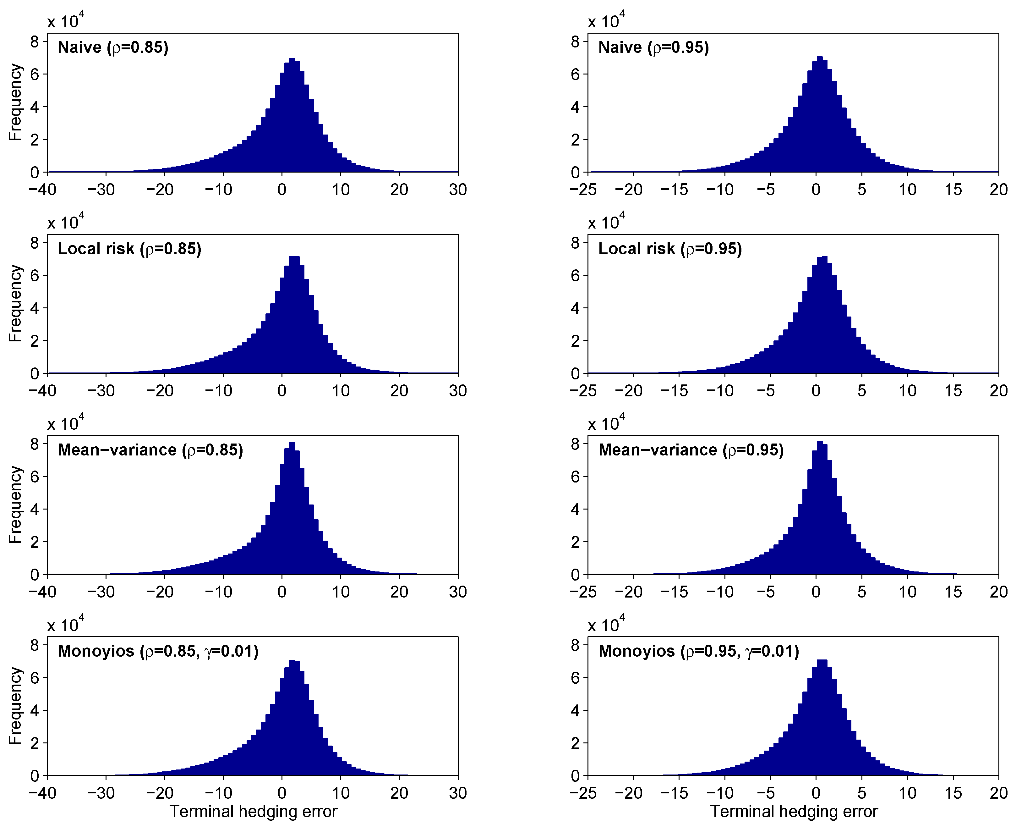
The results are encouraging, with the local risk-minimizing strategy performing at least as well as the Monoyios algorithm (i.e., higher mean/median profit and lower standard deviation). This is not surprising, since for small values of γ the utility formulation is close to the local risk-minimizing strategy. The mean-variance optimal strategy performed slightly better than the other two, with a standard deviation that was 1%–2% lower. This can be seen as an enhanced peak around the mean in the relevant histograms. One slight drawback of this method is that its largest losses exceeded the largest losses of the other methods. The naive strategy performed surprisingly well (certainly significantly better than the naive strategy in Monoyios’ simulations). This is due to the fact that, under the choice of parameters used, the CAPM equilibrium condition is not unreasonable.

Table Table 4 shows the approximation prices for various values of the correlation coefficient, for both put and call options, based on the parameters presented in Table 1. It is interesting to note that the approximation prices for the put are lower than the Black–Scholes prices, while the converse is true for the call. One should not interpret these prices as the premiums charged for the options, since not all risk is hedged, due to incompleteness. It is therefore necessary to estimate the standard deviation of the hedging error, so that the option writer can charge an appropriate risk premium.

Table 4. Put and call option approximation prices for various values of ρ. (For $\rho =1$, they are Black–Scholes prices.)

ρ	Put	Call
−0.95	5.3127	23.7315
−0.75	5.6321	22.6965
−0.50	6.0493	21.4435
−0.25	6.4870	20.2358
0	6.9451	19.0730
0.25	7.4238	17.9549
0.50	7.9231	16.8812
0.75	8.4428	15.8514
0.95	8.8733	15.0588
1	9.3542	14.2312

Table 4. Put and call option approximation prices for various values of ρ. (For $\rho =1$, they are Black–Scholes prices.)

ρ	Put	Call
−0.95	5.3127	23.7315
−0.75	5.6321	22.6965
−0.50	6.0493	21.4435
−0.25	6.4870	20.2358
0	6.9451	19.0730
0.25	7.4238	17.9549
0.50	7.9231	16.8812
0.75	8.4428	15.8514
0.95	8.8733	15.0588
1	9.3542	14.2312

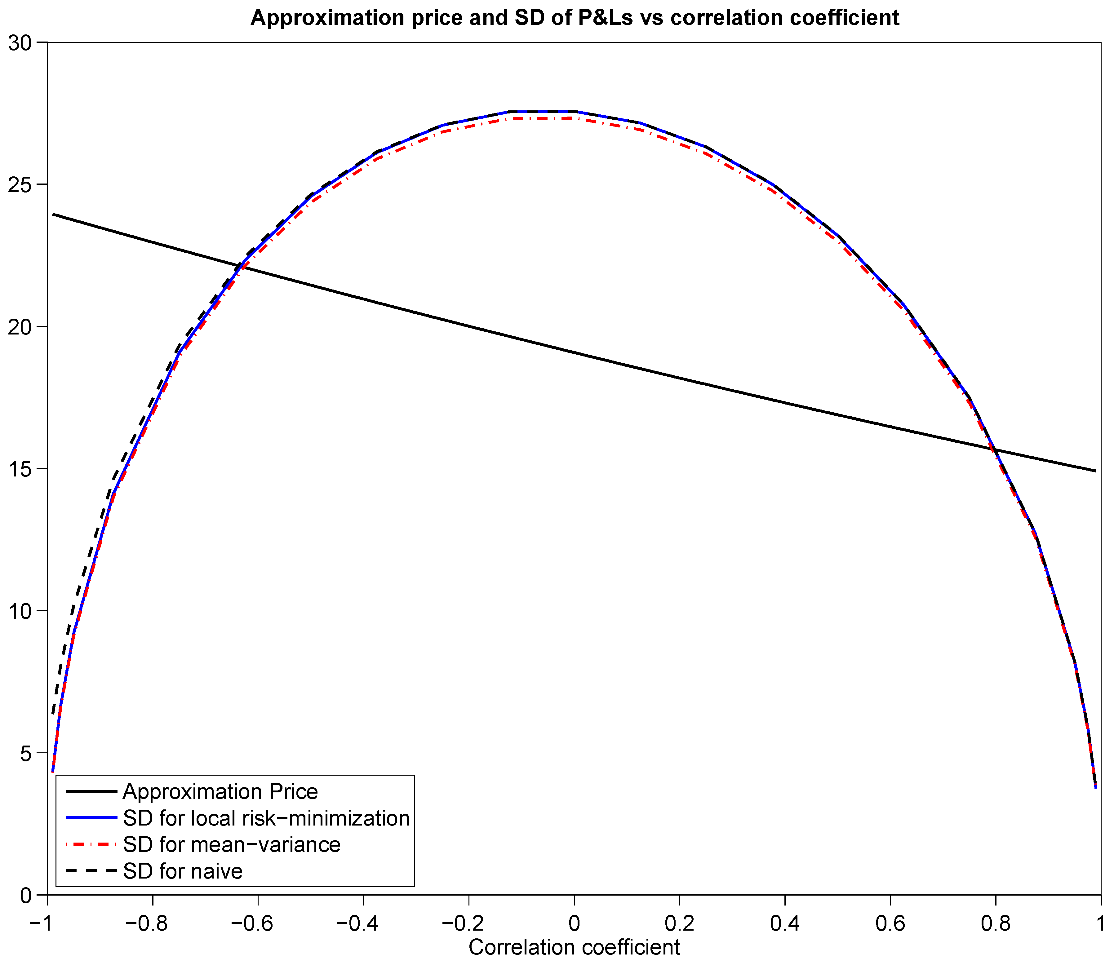
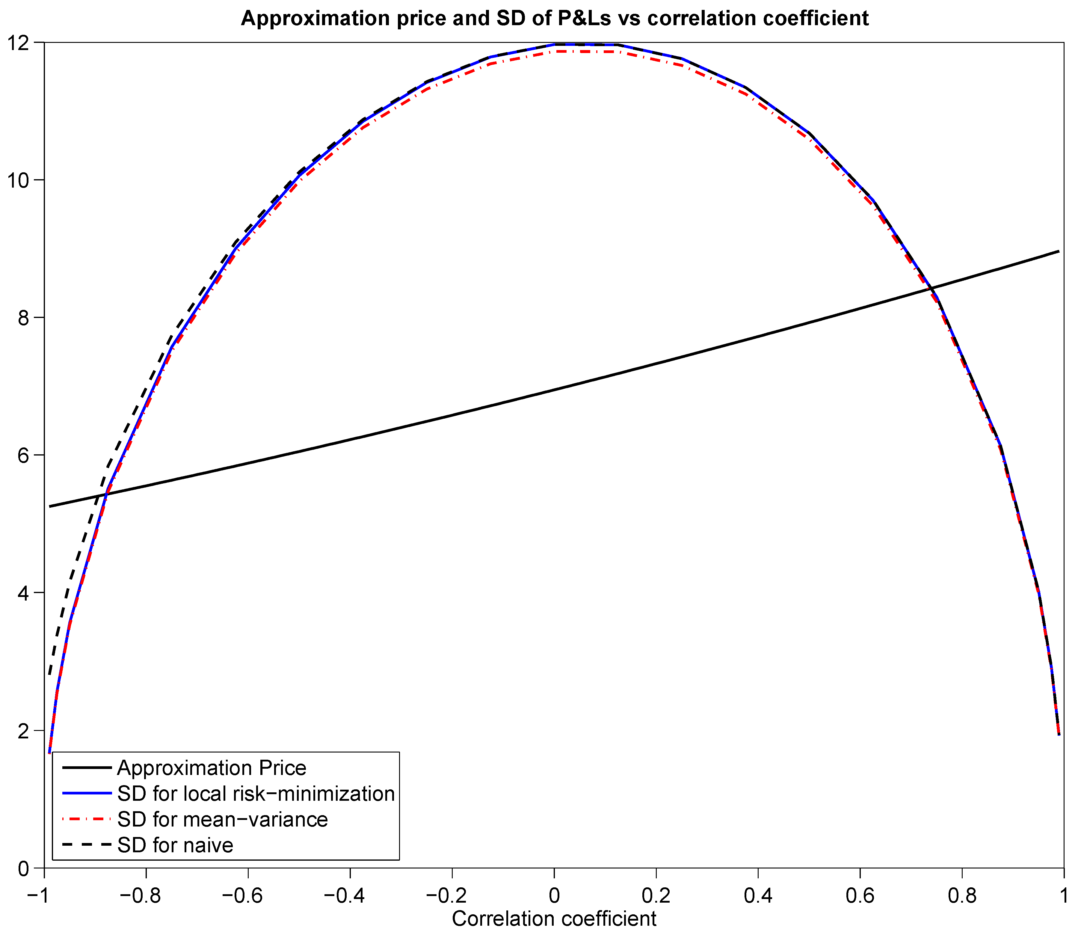
Figure 2 shows the approximation prices and standard deviations of hedging errors for the put, using the naive, local risk-minimizing and mean-variance optimal hedging strategies. Figure 3 shows the same results for the call. The standard deviations were estimated based on Monte Carlo samples of 100,000 paths. We see from these graphs that hedging basis risk is only viable when the assets are highly correlated (in absolute value), since the error in hedging increases rapidly as the correlation between the assets decreases. It is interesting to note that the naive strategy performs very well for correlations close to unity. As the correlation coefficient reduces and becomes negative, it becomes less and less effective, however. This is due to the fact that, under the asset parameters used, the CAPM equilibrium assumption becomes less realistic as the correlation decreases.

Figure 2. Approximation price and standard deviation of hedging error vs. correlation, for the put option with parameters given by Table 1.

Figure 2. Approximation price and standard deviation of hedging error vs. correlation, for the put option with parameters given by Table 1.

10. Conclusions

In this paper we used quadratic criteria to derive simple hedging rules for minimizing basis risk. These rules are considerably simpler than the hedging rules based on utility maximization and perform slightly better in terms of minimizing risk. Their simplicity is a consequence of the fact that they are based on the Black–Scholes formula. By contrast, the utility maximization approach requires the use of series expansions in order to solve the relevant PDEs, which were originally derived using a “distortion” technique. It is important to note that all hedging schemes are only effective when the traded and non-traded assets are highly correlated (in absolute value), thus confirming the sobering conclusions of Davis [2].

As is usual in incomplete market settings, the solutions depend on estimating the growth rates of the assets—a task recognized to be very difficult. In order to address this issue, we have derived a naive hedging strategy that does not depend on the drift parameters. However, this comes with an implicit drawback—the performance of the strategy is dependent on how well a CAPM equilibrium condition is obeyed. In order to establish if this assumption is reasonable, in the context of specific real-world applications, further investigation is required.

Figure 3. Approximation price and standard deviation of hedging error vs. correlation, for the call option with parameters given by Table 1.

Figure 3. Approximation price and standard deviation of hedging error vs. correlation, for the call option with parameters given by Table 1.

References

- M.H.A. Davis. “Option Valuation and Hedging with Basis Risk.” In System Theory: Modeling, Analysis and Control. Edited by T.E. Djaferis and I.C. Schuck. New York, NY, USA: Kluwer, 1999, pp. 245–254. [Google Scholar]
- M.H.A. Davis. “Option Hedging with Basis Risk.” In From Stochastic Calculus to Mathematical Finance. Edited by Y. Kabanov, R. Liptser and J. Stoyanov. Berlin, Germany: Springer, 2006, pp. 169–187. [Google Scholar]
- V. Henderson. “Valuation of Claims on Nontraded Assets Using Utility Maximization.” Math. Financ. 12 (2002): 351–373. [Google Scholar] [CrossRef]
- V. Henderson, and D.G. Hobson. “Substitute Hedging.” Risk 15 (2002): 71–75. [Google Scholar]
- M. Monoyios. “Performance of Utility-Based Strategies for Hedging Basis Risk.” Quant. Financ. 4 (2004): 245–255. [Google Scholar] [CrossRef]
- M. Monoyios. “Optimal hedging and parameter uncertainty.” IMA J. Manag. Math. 18 (2007): 331–351. [Google Scholar] [CrossRef]
- T. Zariphopoulou. “A solution approach to valuation with unhedgeable risks.” Financ. Stoch. 5 (2001): 61–82. [Google Scholar] [CrossRef]
- M. Schweizer. “Mean-Variance Hedging for General Claims.” Ann. Appl. Probab. 2 (1992): 171–179. [Google Scholar] [CrossRef]
- D. Duffie, and H.R. Richardson. “Mean-variance Hedging in Continuous Time.” Ann. Appl. Probab. 1 (1991): 1–15. [Google Scholar] [CrossRef]
- H. Pham. “On Quadratic Hedging in Continuous Time.” Math. Methods Oper. Res. 51 (2000): 315–339. [Google Scholar] [CrossRef]
- M. Schweizer. “A Guided Tour through Quadratic Hedging Approaches.” In Option Pricing, Interest Rates and Risk Management. Edited by E. Jouini, J. Cvitanić and M. Musiela. Cambridge, UK: Cambridge University Press, 2001, Chapter 15; pp. 538–574. [Google Scholar]
- T.A. McWalter. “Quadratic Criteria for Optimal Martingale Measures in Incomplete Markets.” M.Sc. Dissertation; Witwatersrand, South Africa: University of the Witwatersrand, 2006. http://hdl.handle.net/10539/2084 (accessed on 29 January 2015).
- J.M. Harrison, and S.R. Pliska. “Martingales and Stochastic Integrals in the Theory of Continuous Trading.” Stoch. Process. Their Appl. 11 (1981): 215–260. [Google Scholar] [CrossRef]
- J.M. Harrison, and S.R. Pliska. “A Stochastic Calculus Model of Continuous Trading: Complete Markets.” Stoch. Process. Their Appl. 15 (1983): 313–316. [Google Scholar] [CrossRef]
- M. Schweizer. “Risk-minimality and orthogonality of martingales.” Stoch. Stoch. Rep. 30 (1990): 123–131. [Google Scholar] [CrossRef]
- M. Schweizer. “Option hedging for Semimartingales.” Stoch. Process. Their Appl. 37 (1991): 339–363. [Google Scholar] [CrossRef]
- H. Föllmer, and M. Schweizer. “Hedging of Contingent Claims Under Incomplete Information.” In Applied Stochastic Analysis. Edited by M.H.A. Davis and R.J. Elliott. New York, NY, USA: Gorden and Breach Science Publishers, 1991, pp. 389–414. [Google Scholar]
- M. Schweizer. “On the minimal martingale measure and the Föllmer-Schweizer decomposition.” Stoch. Anal. Appl. 13 (1995): 573–599. [Google Scholar] [CrossRef]
- D. Heath, E. Platen, and M. Schweizer. “A Comparison of Two Quadratic Approaches to Hedging in Incomplete Markets.” Math. Financ. 11 (2001): 385–413. [Google Scholar] [CrossRef]
- N. El Karoui, S. Peng, and M.C. Quenez. “Backward Stochastic Differential Equations in Finance.” Math. Financ. 7 (1997): 1–71. [Google Scholar] [CrossRef]
- S.E. Shreve. Stochastic Calculus for Finance II: Continuous-Time Models. New York, NY, USA: Springer-Verlag, 2004. [Google Scholar]
- L.C.G. Rogers. “The relaxed investor and parameter uncertainty.” Financ. Stoch. 5 (2001): 131–154. [Google Scholar] [CrossRef]
- M. Monoyios. “Utility-based valuation and hedging of basis risk with partial information.” Appl. Math. Financ. 17 (2010): 519–551. [Google Scholar] [CrossRef]
- D.G. Luenberger. Investment Science. New York, NY, USA: Oxford University Press, 1998. [Google Scholar]
© 2015 by the authors; licensee MDPI, Basel, Switzerland. This article is an open access article distributed under the terms and conditions of the Creative Commons Attribution license (http://creativecommons.org/licenses/by/4.0/).
Share and Cite
MDPI and ACS Style
Hulley, H.; McWalter, T.A. Quadratic Hedging of Basis Risk. J. Risk Financial Manag. 2015, 8, 83-102. https://doi.org/10.3390/jrfm8010083
AMA Style
Hulley H, McWalter TA. Quadratic Hedging of Basis Risk. Journal of Risk and Financial Management. 2015; 8(1):83-102. https://doi.org/10.3390/jrfm8010083
Chicago/Turabian StyleHulley, Hardy, and Thomas A. McWalter. 2015. "Quadratic Hedging of Basis Risk" Journal of Risk and Financial Management 8, no. 1: 83-102. https://doi.org/10.3390/jrfm8010083