
Pricing a Collateralized Derivative Trade with a Funding Value Adjustment

Abstract
:1. Introduction
2. The CRR Model with Collateral and Dividends
- the rate paid on collateral,
- the rate paid on a repurchase agreement of non-dividend paying stock,
- the rate paid on unsecured funding, and
- the dividend yield on the stock.
- Δ amount of stock, and
- γ amount of cash.
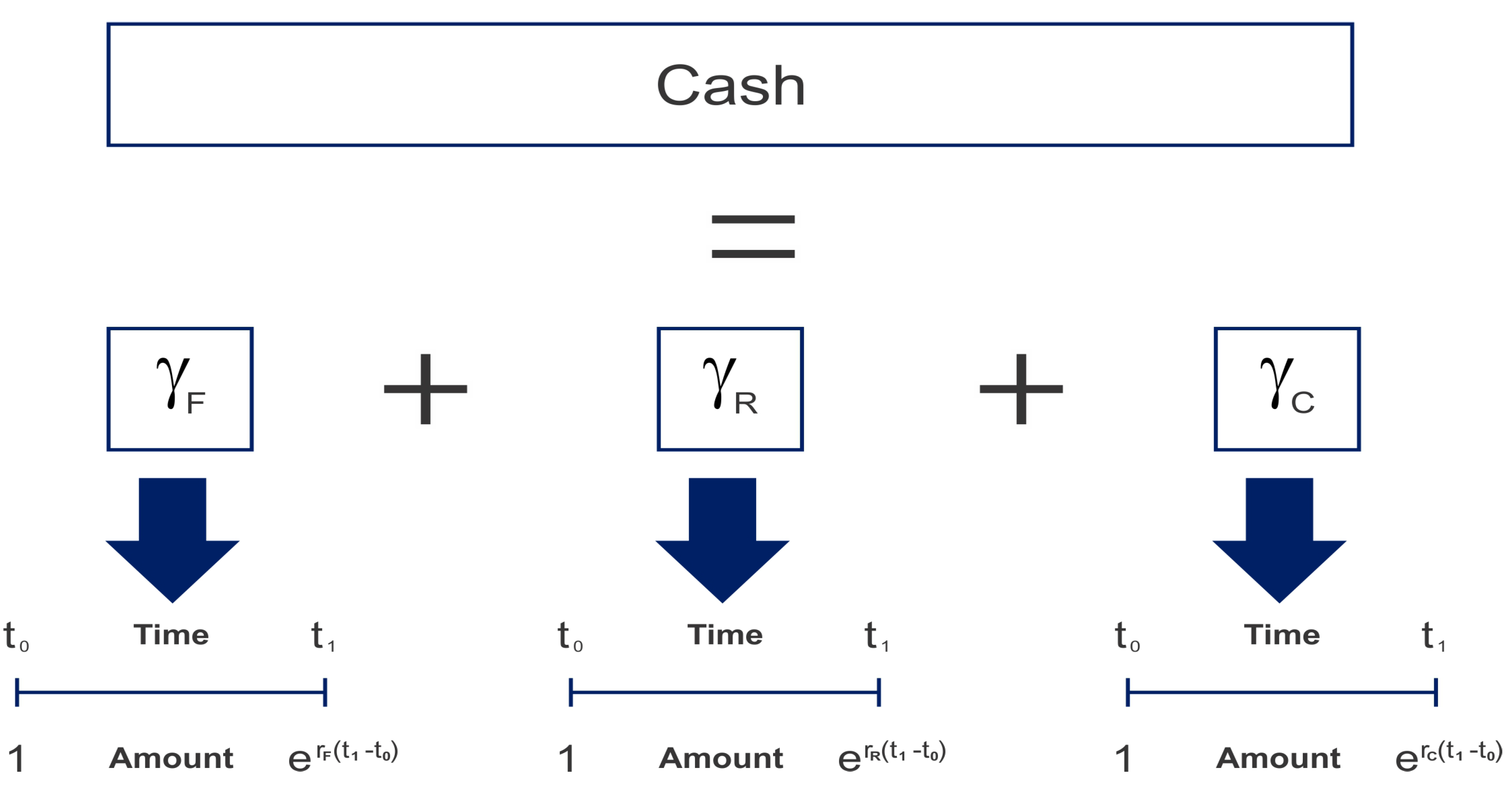
2.1. Cash Account of the CRR Model with Collateral
- The amount in the funding account is denoted by . This amount is the difference between two cash amounts, namely the price of the hedging portfolio and the collateral amount. The cash price of the hedging portfolio is denoted by , and the collateral amount is denoted by ; hence . This amount is the amount needed to be borrowed or lent at the unsecured funding rate, . The model makes the assumption that one can borrow or lend cash out at the funding rate without incurring counterparty credit risk.
- The amount in the repo account is denoted by . This account consists of the cash invested or borrowed in order to fund the stock position, , through a repurchase agreement.
- The amount in the collateral account is denoted by . This account contains the collateral posted with the counterparty. This account grows at the collateral rate . The assumptions made about the posted collateral in this model are that no hair cut is applied to the collateral value and that the currency of the collateral and the settlement of the derivative are the same.

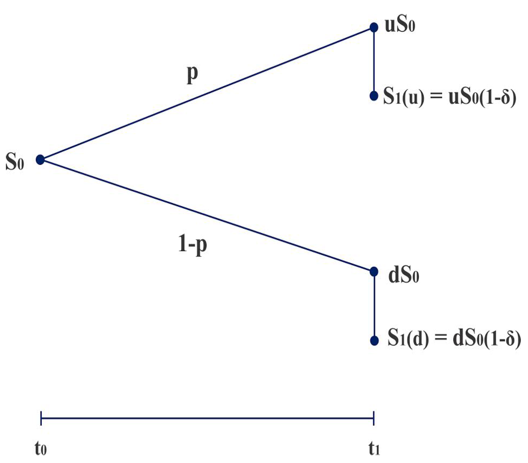
2.2. One Period Binomial Model with Collateral

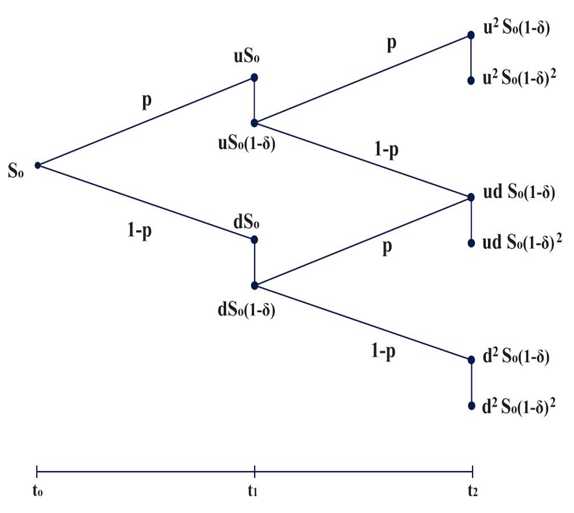
2.3. n-Period Binomial Model with Collateral

3. Collateral and Determining a Discount Factor
3.1. Partial Collateralization
4. Black-Scholes-Merton PDE with Collateral and Dividends
5. Discretizing the Piterbarg Model Yields the CRR Model with Collateral
- is continuous, is of class and satisfies the Cauchy problem:where the function is the final payoff of the derivative contract and is the stock process, and
- also satisfies the polynomial growth condition:for some .
6. Numerical Implementation
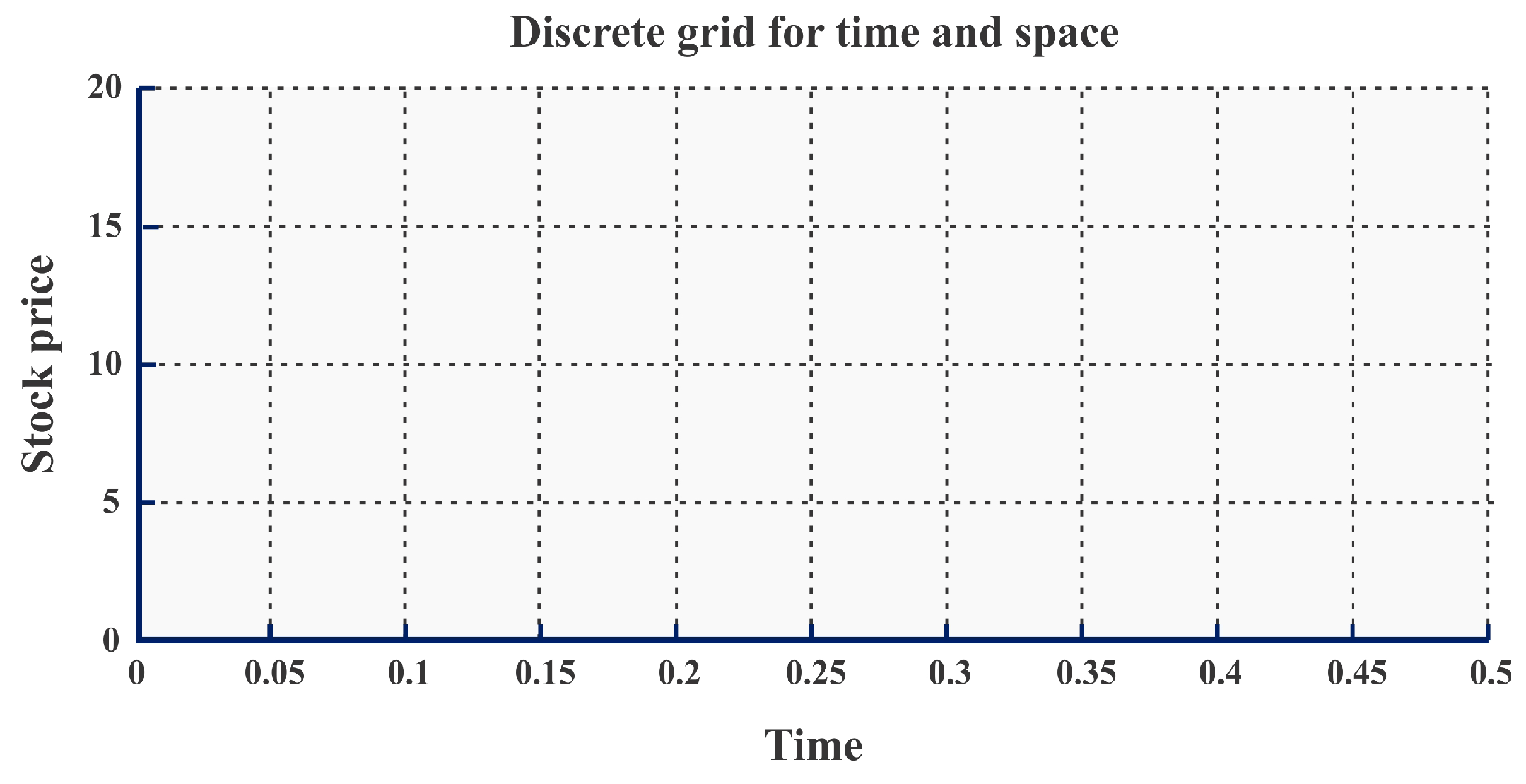
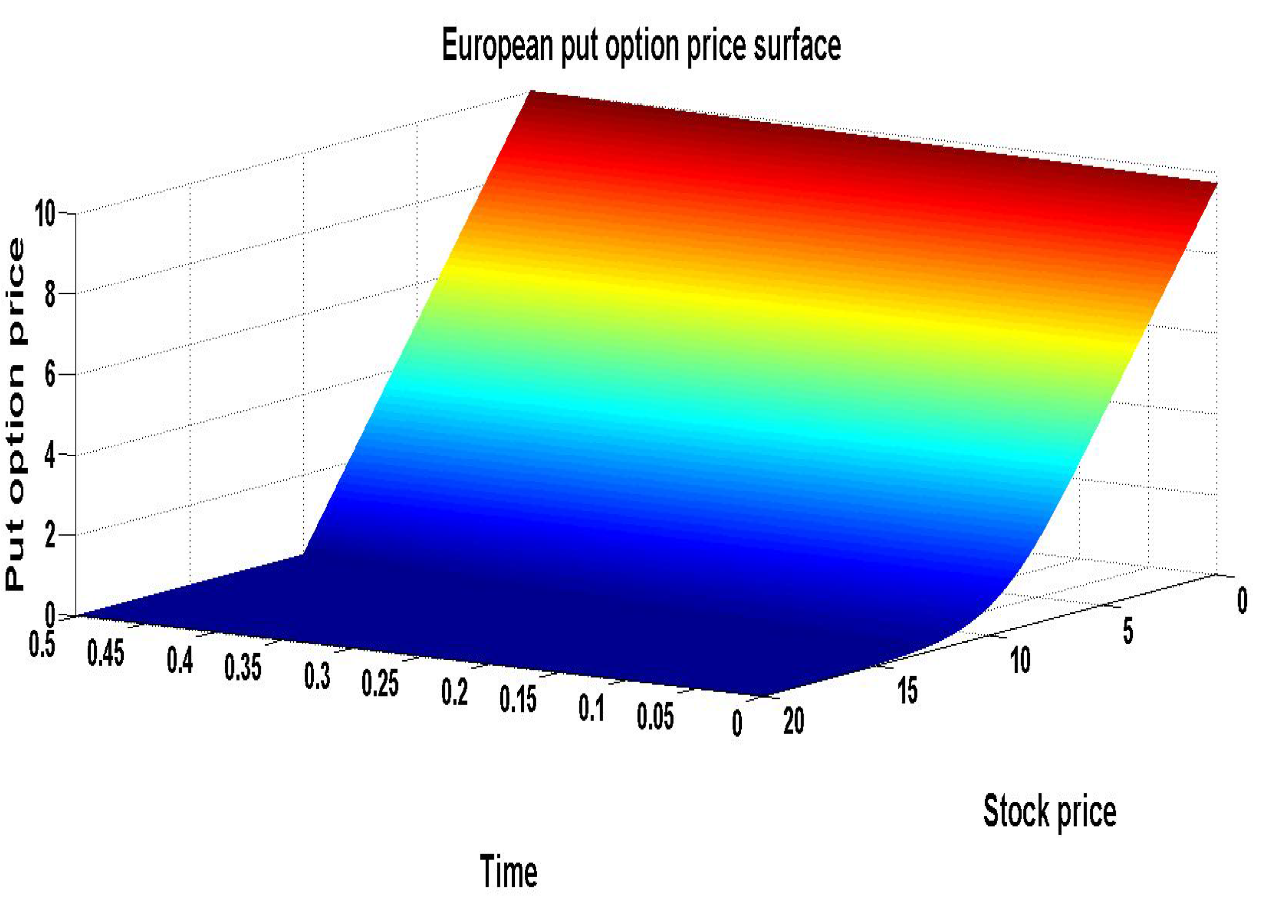
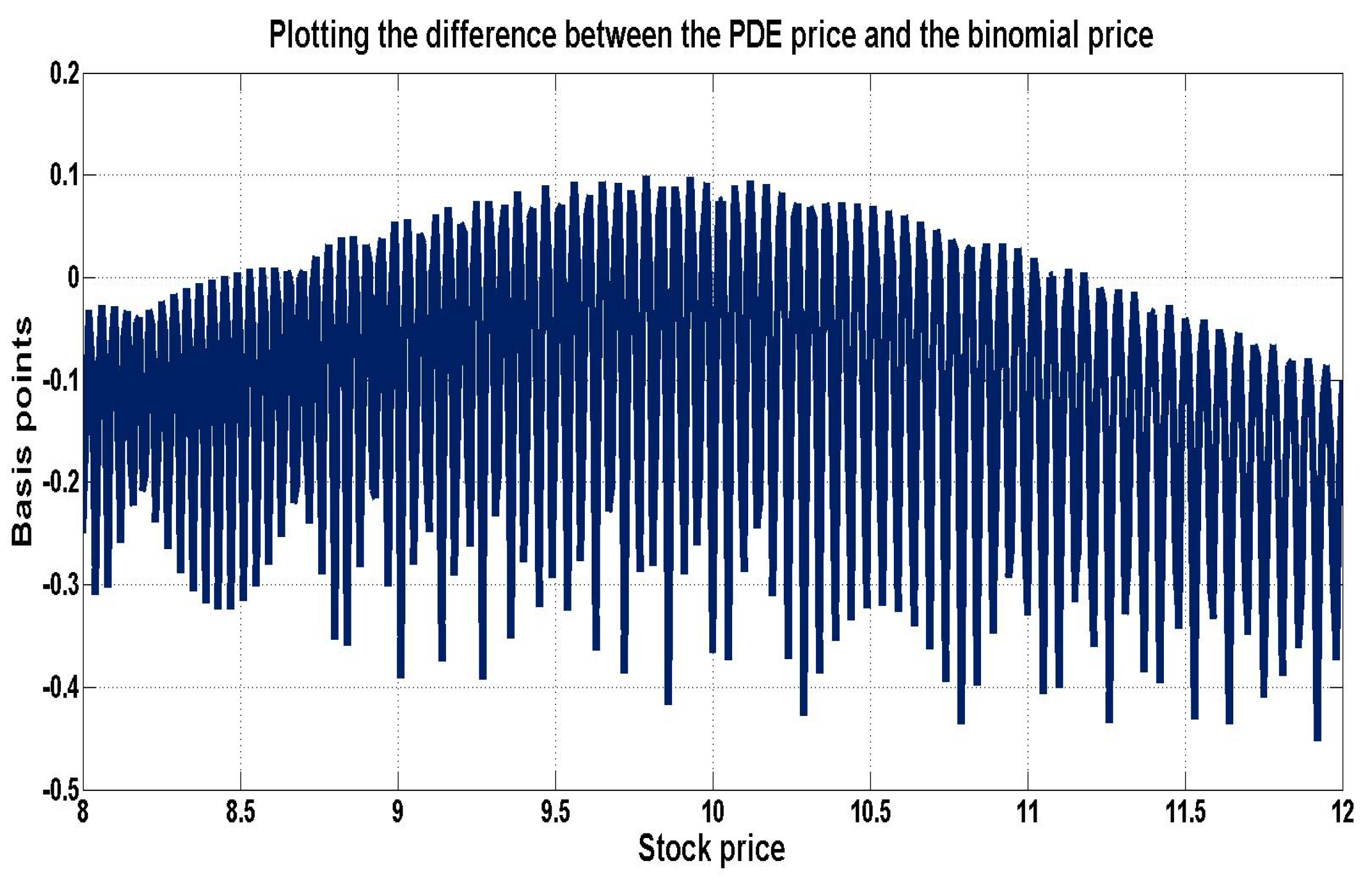
6.1. PDE Approach
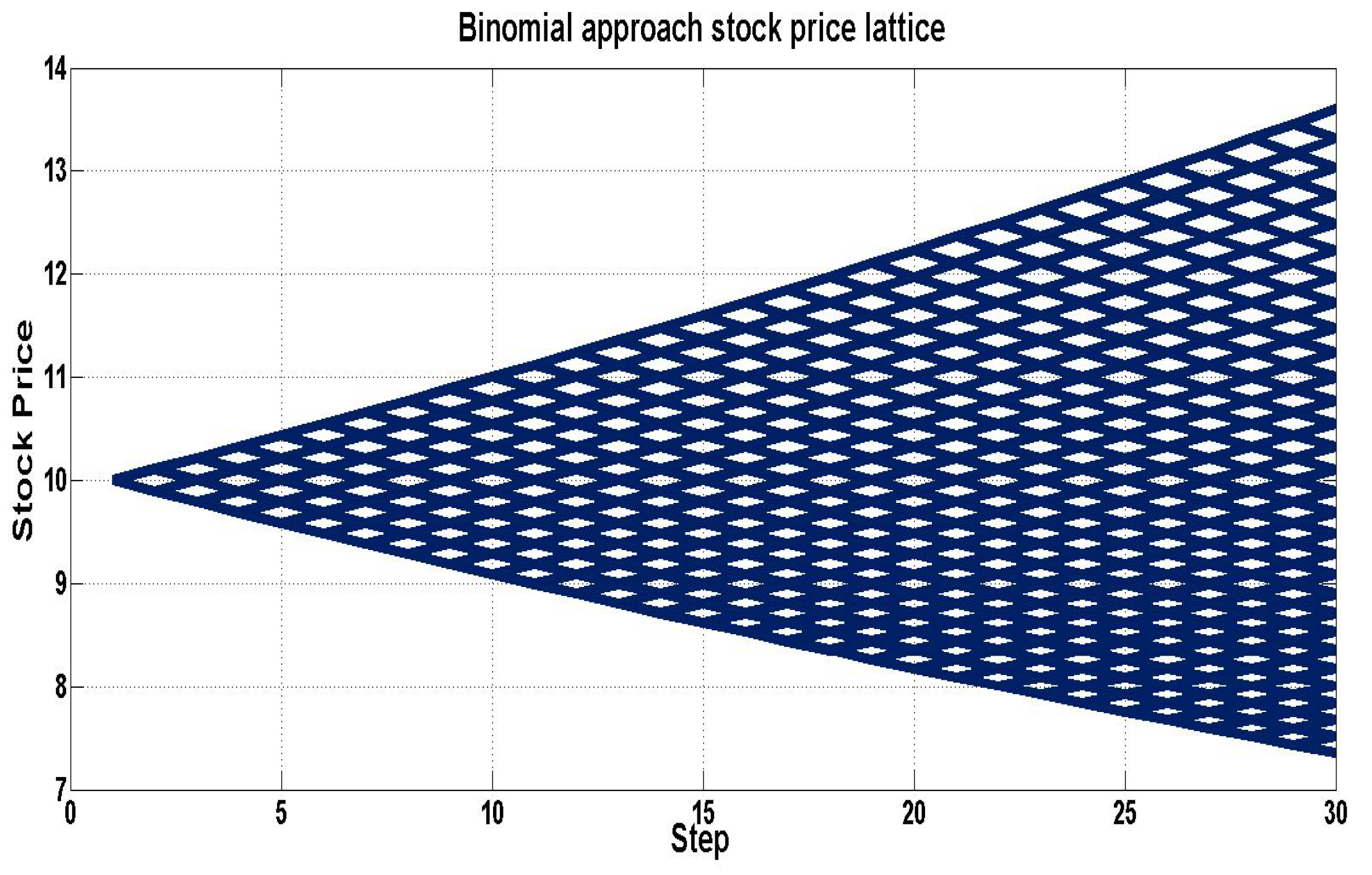
6.2. Binomial Lattice Approach


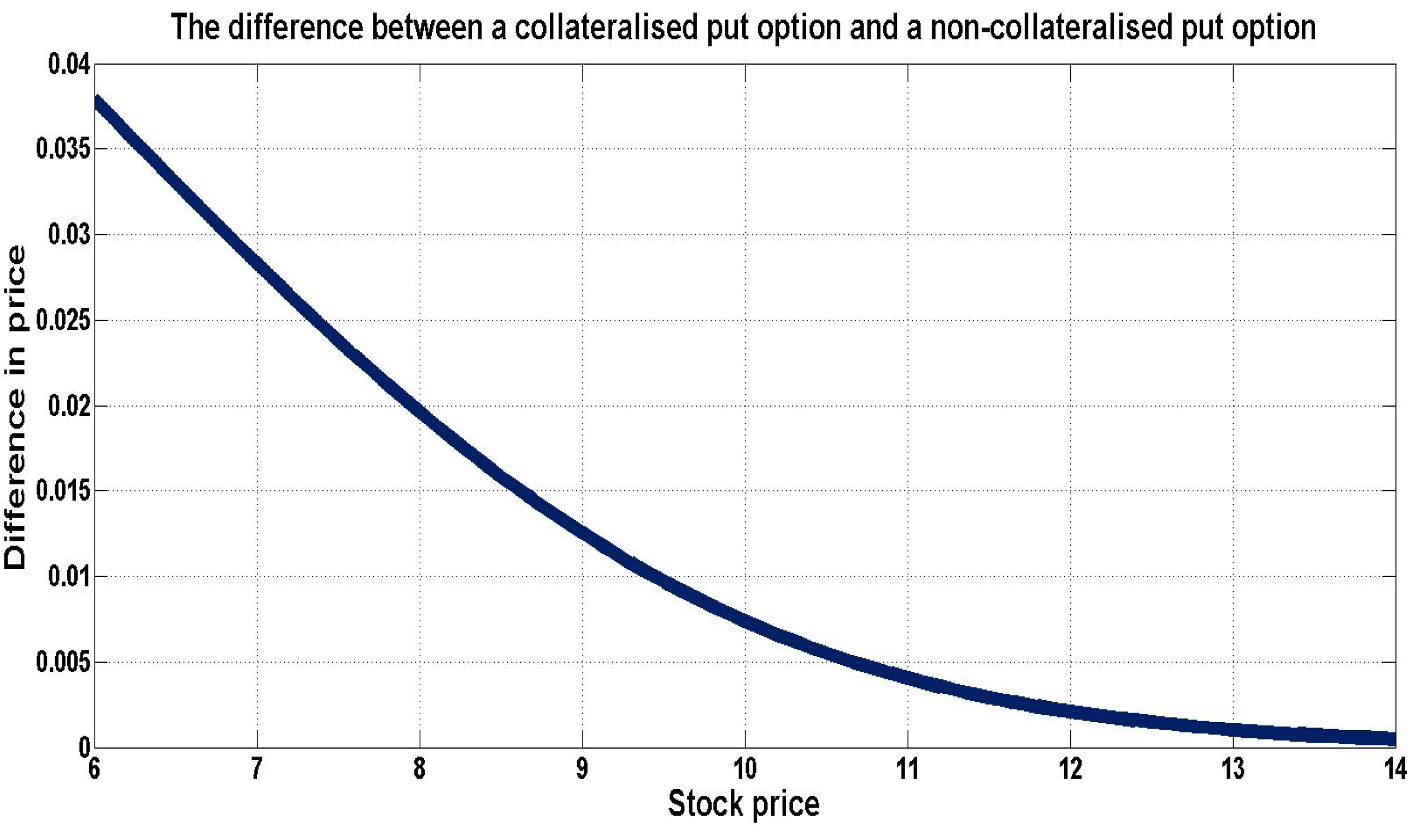
| European Put Option | PDE Price | Binomial Lattice Price |
|---|---|---|
| Full collateral | 0.741011 | 0.740992 |
| No collateral | 0.733637 | 0.733619 |
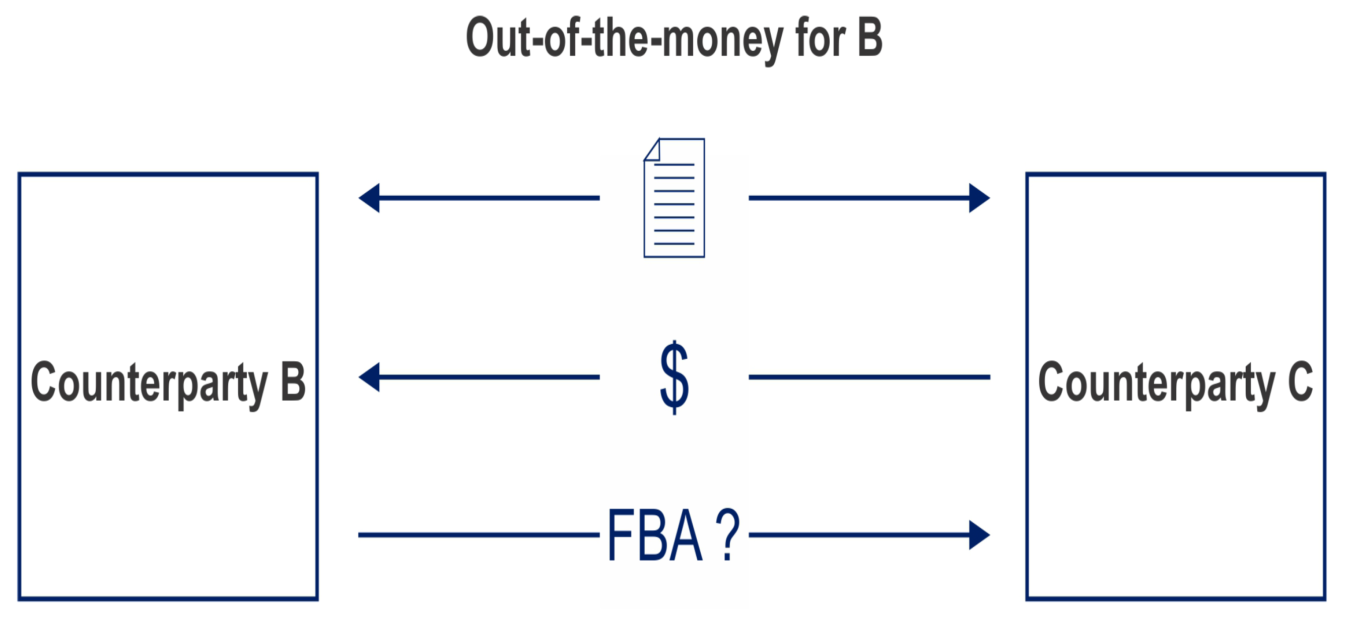
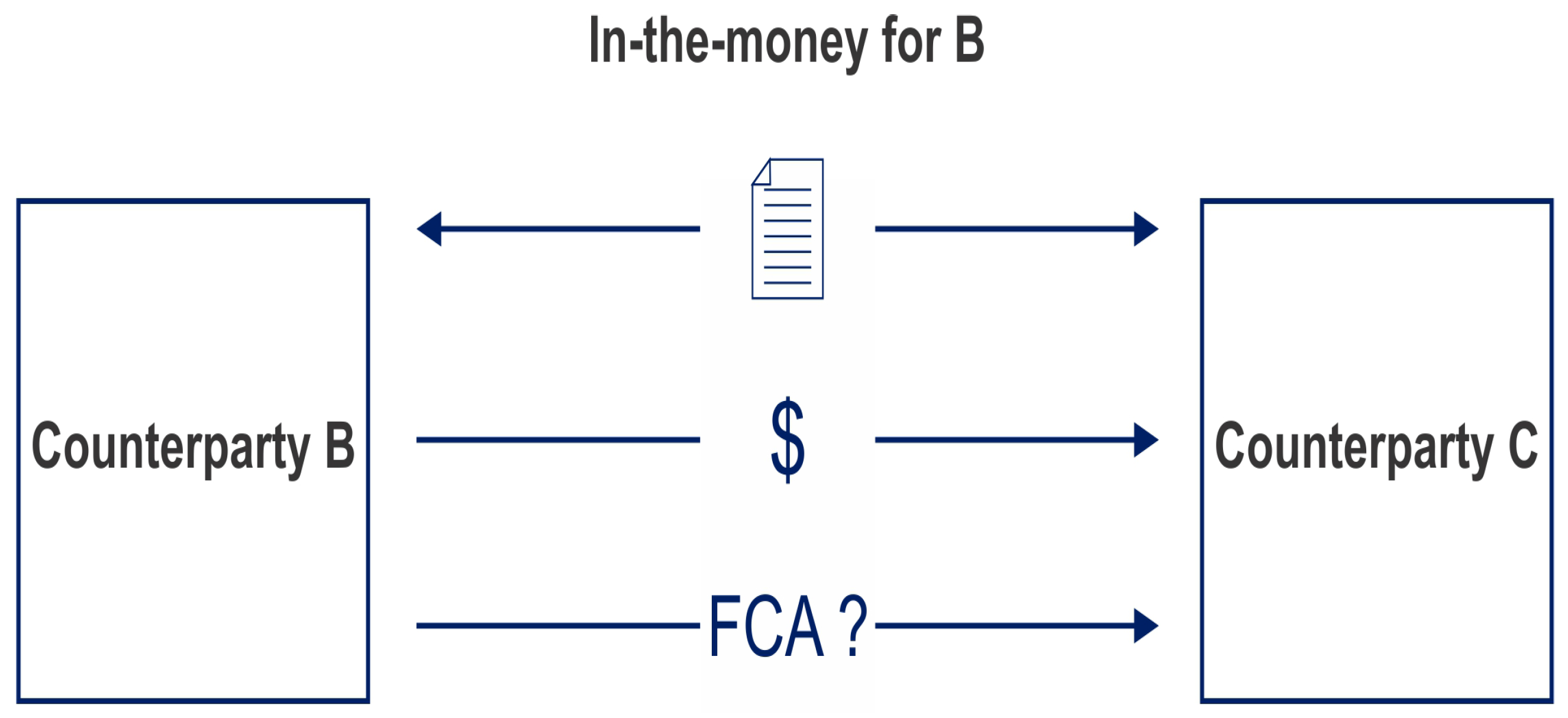
| FCA | −0.007374 | −0.007372 |
6.3. Default Risk Caused by Readjusting Collateral at Discrete Times

7. Conclusions
Acknowledgments
Author Contributions
Appendix: Derivations
A. Solving the Piterbarg PDE Numerically
B. Deriving the Parameters for the Binomial Asset Pricing Model
Conflicts of Interest/Disclaimer
References
- J. Hull, and A. White. “LIBOR vs. OIS: The derivatives discounting dilemma.” J. Invest. Manag. 11 (2013): 14–27. [Google Scholar]
- J. Gregory. Counterparty Credit Risk and Credit Value Adjustment—A Continuing Challenge for Global Financial Markets, 2nd ed. London, UK: Wiley & Sons Ltd., 2012. [Google Scholar]
- C. Hunzinger, and C.C.A. Labuschagne. “The Cox, Ross and Rubinstein tree model which includes counterparty credit risk and funding costs.” North Am. J. Econ. Financ. 29 (2014): 200–217. [Google Scholar] [CrossRef]
- J. Hull, and A. White. “The FVA debate.” Risk Mag. 25 (2012): 83–85. [Google Scholar]
- V. Piterbarg. “Funding beyond discounting: Collateral agreements and derivatives pricing.” Risk Mag. 23 (2010): 97–102. [Google Scholar]
- J. Hull, and A. White. “Valuing derivatives: Funding value adjustments and fair value.” Financ. Anal. J. 70 (2014): 46–56. [Google Scholar] [CrossRef]
- V. Piterbarg. “Cooking with collateral.” Risk Mag. 25 (2010): 58–63. [Google Scholar]
- S. Laughton, and A. Vaisbrot. “In defence of FVA.” Risk Mag. 25 (2012): 18–24. [Google Scholar]
- J. Cox, S. Ross, and M. Rubinstein. “Option pricing: A simplified approach.” J. Financ. Econ. 7 (1979): 229–263. [Google Scholar] [CrossRef]
- S. Shreve. Stochastic Calculus for Finance 1—The Binomial Asset Pricing Model, 1st ed. New York, NY, USA: Springer, 2004. [Google Scholar]
- K. Itô. “Stochastic integral.” Proc. Imp. Acad. Tokyo 20 (1944): 519–524. [Google Scholar] [CrossRef]
- K. Itô. “On stochastic differential equations.” Mem. Am. Math. Soc. 4 (1951): 1–51. [Google Scholar]
- J. Björk. Arbitrage Theory in Continuous Time, 2nd ed. New York, NY, USA: Oxford University Press Inc., 2004. [Google Scholar]
- I. Karatzas, and S.E. Shreve. Brownian Motion and Stochastic Calculus, 2nd ed. New York, NY, USA: Springer, 1991. [Google Scholar]
- P. Brandimarte. Numerical Methods in Finance & Economics, 2nd ed. New Jersey, NJ, USA: John Wiley & Sons Publications, 2006. [Google Scholar]
- M. Richardson. “Numerical Methods for Option Pricing.” PhD Thesis, Mathematical Institute, University of Oxford, Oxford, UK, 2009. [Google Scholar]
- D. Higham. An Introduction to Financial Option Valuation. Cambridge, UK: Cambridge University Press, 2008. [Google Scholar]
- J. Hull, and A. White. “Collateral and credit issues in derivatives pricing. Forthcoming.” J. Credit Risk. [CrossRef]
- C. Burgard, and M. Kjaer. “Partial differential equation representations of derivatives with bilateral counterparty risk and funding costs.” J. Credit Risk 7 (2011): 75–93. [Google Scholar] [CrossRef]
- C. Burgard, and M. Kjaer. “Generalised CVA with funding and collateral via semi-replication. ” [CrossRef]
- KPMG. “Challenges facing the South African derivatives market.” In Bank Survey Report. Johannesburg, South Africa: KPMG, 2013. [Google Scholar]
- 1.Here, means that the first partial derivative with respect to time of the function is continuous and that the second derivative of the function with respect to the space variable, i.e., , is also continuous.
- 2.The filtration is not included in the expectation operator for ease of notation. The subscript in the conditional expectation, i.e., , indicates that the expectation is conditioned on the filtration at time t.
© 2015 by the authors; licensee MDPI, Basel, Switzerland. This article is an open access article distributed under the terms and conditions of the Creative Commons Attribution license (http://creativecommons.org/licenses/by/4.0/).
Share and Cite
Hunzinger, C.B.; Labuschagne, C.C.A. Pricing a Collateralized Derivative Trade with a Funding Value Adjustment. J. Risk Financial Manag. 2015, 8, 17-42. https://doi.org/10.3390/jrfm8010017
Hunzinger CB, Labuschagne CCA. Pricing a Collateralized Derivative Trade with a Funding Value Adjustment. Journal of Risk and Financial Management. 2015; 8(1):17-42. https://doi.org/10.3390/jrfm8010017
Chicago/Turabian StyleHunzinger, Chadd B., and Coenraad C.A. Labuschagne. 2015. "Pricing a Collateralized Derivative Trade with a Funding Value Adjustment" Journal of Risk and Financial Management 8, no. 1: 17-42. https://doi.org/10.3390/jrfm8010017