Conserving Capital by Adjusting Deltas for Gamma in the Presence of Skewness

Robert H. Smith School of Business, University of Maryland, College Park, MD. 20742, USA
J. Risk Financial Manag. 2010, 3(1), 1-25; https://doi.org/10.3390/jrfm3010001
Published: 31 December 2010
Abstract
:An argument for adjusting Black Scholes implied call deltas downwards for a gamma exposure in a left skewed market is presented. It is shown that when the objective for the hedge is the conservation of capital ignoring the gamma for the delta position is expensive. The gamma adjustment factor in the static case is just a function of the risk neutral distribution. In the dynamic case one may precompute at the date of trade initiation a matrix of delta levels as a function of the underlying for the life of the trade and subsequently one just has to look up the matrix for the hedge. Also constructed are matrices for the capital reserve, the profit, leverage and rate of return remaining in the trade as a function of the spot at a future date in the life of the trade. The concepts of profit, capital, leverage and return are as described in Carr, Madan and Vicente Alvarez (2010). The dynamic computations constitute an application of the theory of nonlinear expectations as described in Cohen and Elliott (2010).
Keywords:
Bid and Ask Prices; Concave Distortions; Non Linear Expectations; Variance Gamma Model; Non-Uniform GridsJEL Classification:
G131 INTRODUCTION
We shall show that in the interests of conserving capital in markets where delta hedging leaves one exposed to residual risk one may wish to adjust one’s delta position in line with position’s gamma. When markets are complete as in the case of a diffusion for the underlying risk, the risk in a position’s gamma is perfectly compensated by the theta and the resulting local cash flow is transformed into a riskless exposure. More generally, in the presence of numerous jump possibilities, for all levels of theta, a long delta position is exposed in left skewed markets to losses of down moves in proportion to the position gamma. Inorder to reduce the capital cost of these exposures one may wish to reduce the delta in line with the gamma. Similarly, a short delta position is induced to tilt the delta to a higher short position to access downside gains thereby conserving capital. These intuitions will be made precise and verified here. The result is the recommendation of a gamma adjustment to delta hedging that responds to the underlying volatility and the market skew.
We first work in a static single period context defining capital, profits, leverage and returns as in Carr, Madan and Vicente Alvarez (2010) and show how capital conservation strategies lead to gamma adjustments for the delta. The static model presented builds on the theory of two price markets developed in Cherny and Madan (2010) that gave us operational procedures for determining bid and ask prices. These prices are by construction concave and convex functionals on the space of bounded random variables and hence they are nonlinear. We go on to employ the fast developing theory of nonlinear expectations (Peng (2004), Rosazza Gianin (2006), Delbaen, Peng, Rosazza Gianin (2010), Jobert and Rogers (2008), Cohen and Elliott (2010)) to construct dynamically consistent sequences of bid and ask prices that result in dynamic gamma adjusted delta hedging strategies. These are implemented and compared to delta hedging at the Black Scholes implied volatility when the underlying risk is that of a Lévy process. Significant levels of capital conservation are seen to result from the use of a gamma adjustment.
The outline of the rest of the paper is as follows. Section 2 briefly presents the static concepts of profit, capital, leverage and return. Section 3 investigates in the static context the benefits of the proposed gamma adjustment. Section 4 discusses the use of nonlinear expectations in a multiperiod context. Section 5 develops dynamic hedging for capital conservation. These are implemented on a one year out of the money call and put option and the results are reported. Section 6 concludes.
2 THE ONE PERIOD MODEL
We begin with the model of a market as a counterparty as described in Cherny and Madan (2010). The market is modeled by describing the bounded random variables the market will accept at zero cost to it. In keeping with classical finance where market participants may trade arbitrary sizes with the market, it is observed that this set of random variables acceptable to the market at zero cost must be a convex cone that contains the nonnegative random variables. As a result (Artzner, Delbaen, Eber and Heath (1999)) one may associate with each such set a convex set of probability measures equivalent to the original measure P such that X is acceptable to the market at zero cost if and only if
![Jrfm 03 00001 i001]()

The set is referred to as test scenarios in Carr, Geman and Madan (2001) and supporting measures in Cherny and Madan (2009, 2010). Related literature includes Jaschke and Küchler (2001), and Černý and Hodges (2000). With a view to keeping the set of acceptable risks strictly smaller than those acceptable in classical finance we suppose, as in Cherny and Madan (2010) that the base or reference measure P is a risk neutral measure and further that P ∈ .
Cherny and Madan (2010) show that for an unhedged risk X to be acceptable to the market the cost of selling X to the market is the bid price b(X) where
![Jrfm 03 00001 i002]()

Similarly the market sells the cash flow X and takes the opposite position −X for the ask price a(X) where
![Jrfm 03 00001 i003]()

In the presence of zero cost hedging assets, where denotes the set of zero cost cash flows to the hedging assets, one defines the risk neutral measures as all measures Q equivalent to P for which EQ[H] = 0, all H ∈ . The bid and ask prices respectively bh(X), ah(X) for the hedged cash flow are respectively
![Jrfm 03 00001 i004]()

One observes that the hedged bid is higher and the ask is lower with a correspondingly narrower spread.
The optimal hedges for the ask price, H and the bid price H are defined by
![Jrfm 03 00001 i005]()

Models defining acceptable cash flows in terms of their distribution functions F(x) were introduced in Cherny and Madan (2010) following Kusuoka (2001) using concave distortions for Ψ(u) a concave distribution function on the unit interval by defining X as acceptable just if
![Jrfm 03 00001 i006]()

The set of supporting measures is identified in Cherny (2006) as all measures Q equivalent to P whose density Z satisfies
![Jrfm 03 00001 i007]()

It is shown in Cherny and Madan (2010) that if we focus on approving distribution functions F(x) or equivalently their inverses G(u) then the supporting measures have densities Z(u) on the unit interval with H(u) ≤ Ψ(u) where H′ = Z. It is shown in Cherny and Madan (2010) that in terms of distortions one may write the unhedged bid and ask prices as
![Jrfm 03 00001 i008]()

Carr, Madan and Vicente Alvarez (2010) express these prices in terms of the inverse distribution function with median, F(m) = 1/2 as
![Jrfm 03 00001 i009]()
![Jrfm 03 00001 i010]()


For hedges H ∈ with hedged distribution functions FH (X) the distribution function for X − H the bid and ask prices are
![Jrfm 03 00001 i011]()
![Jrfm 03 00001 i012]()


The distortion used in Cherny and Madan (2009, 2010) and Carr, Madan and Vicente Alvarez (2010) is minmaxvar defined by
![Jrfm 03 00001 i013]()

We shall continue to use this distortion here.
Given explicitly computable expressions (3) and (4) for the bid and ask prices in the presence of hedges Carr, Madan and Vicente Alvarez (2010) employ these to define the up front profit on a trade, the capital reserve to be taken on the trade and hence the return of the trade. In addition measuring the scale as the expectation of the absolute deviation from the median, leverage is defined as the ratio of the scale to the capital. The upfront profit is defined as the difference between the mid quote and the risk neutral expectation and for options it is observed that this is generally positive. The capital reserve is defined as the cost of going in and out of the trade with the market and hence paying the spread between the ask and bid prices. It is observed from expressions (1) and (2) that the profit π and capital κ are given by
![Jrfm 03 00001 i014]() where H is antisymmetric about 1/2 and is zero at 0, 1/2 and 1, while K is symmetric about 1/2 and specifically
where H is antisymmetric about 1/2 and is zero at 0, 1/2 and 1, while K is symmetric about 1/2 and specifically
![Jrfm 03 00001 i015]()


The return ρ is just π/κ while the leverage λ = scale/κ where the scale is given by
![Jrfm 03 00001 i016]()

3 GAMMA ADJUSTED DELTAS IN LEFT SKEWED MARKETS
We consider here the hedging of quadratic exposures with a view to minimizing the capital charge for the residual risk exposure. Suppose the target cash flow c(S) to be hedged over a time interval of size h is quadratic in the stock price with
![Jrfm 03 00001 i017]()

Consider a hedge position ζ in the stock with a residual cash flow of
![Jrfm 03 00001 i018]()

Suppose the underlying stock price motion x = S − S0 has distribution F(x) and the objective is to minimize the capital required defined by the difference between the ask and bid prices computed using the concave distortion Ψ. To evaluate this capital we need to determine the distribution function of the residual cash flow as both the bid and ask prices are functions of this distribution function. Let C denote the residual cash flow.
The probability FC(v) that C ≤ v is the probability that
![Jrfm 03 00001 i019]()

The minimum cash flow occurs at
![Jrfm 03 00001 i020]() and is equal to
and is equal to
![Jrfm 03 00001 i120]()


Hence
![Jrfm 03 00001 i021]()

For ![Jrfm 03 00001 i076]() we solve for x the equation
we solve for x the equation
![Jrfm 03 00001 i022]() with
with
![Jrfm 03 00001 i023]() and the probability that C ≤ v equals the probability that S − S0 lies between the two solutions. We then have that
and the probability that C ≤ v equals the probability that S − S0 lies between the two solutions. We then have that
![Jrfm 03 00001 i024]()
 we solve for x the equation


We define
![Jrfm 03 00001 i025]() and write
and write
![Jrfm 03 00001 i026]()


The lower bound is now
![Jrfm 03 00001 i027]()

Now −C ≤ γη2/2 and the distribution function for −C is Pr (−C ≤ v) and
![Jrfm 03 00001 i028]() for v < γη2/2 we have that
for v < γη2/2 we have that
![Jrfm 03 00001 i029]() It follows that the ask price is
It follows that the ask price is
![Jrfm 03 00001 i030]() and the bid price is
and the bid price is
![Jrfm 03 00001 i031]() Hence the capital is
Hence the capital is
![Jrfm 03 00001 i032]() Now we make the change of variable
Now we make the change of variable
![Jrfm 03 00001 i033]() to observe that
to observe that
![Jrfm 03 00001 i034]()


For the optimal value for η we just need to minimize the expression for unit γ or we need to minimize
![Jrfm 03 00001 i035]() and this expression just depends on the underlying stock price distribution. One may therefore determine the optimal η from the risk neutral distribution of the stock and then we hedge with gamma adjustment using the delta position
and this expression just depends on the underlying stock price distribution. One may therefore determine the optimal η from the risk neutral distribution of the stock and then we hedge with gamma adjustment using the delta position

ζ = δ − ηγ.
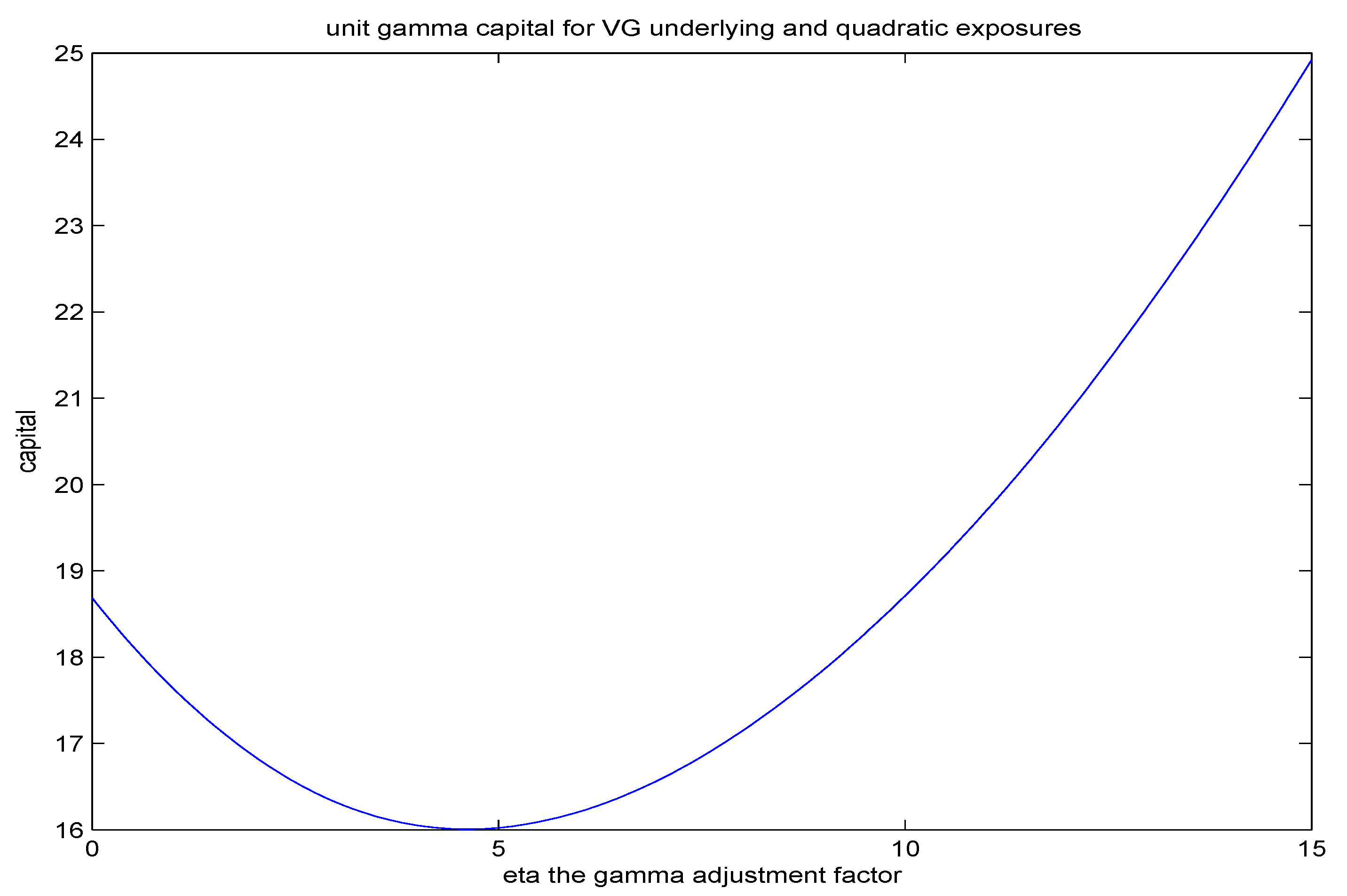
We illustrate the function Λ as a function of η for the variance gamma model (Madan and Seneta (1990), Madan Carr and Chang (1998)) calibrated to options on the SPX on July 15 2010. For weekly monitoring with VG parameters .2196, .3317, −.3596 we graph in Figure (1) the unit gamma capital as a function of the adjustment factor η. The minimum in this case occurs at η = 4.6071.
We observe from this section the basic intuition underlying the gamma adjustment for delta hedging when markets are skewed downwards. Residual risks even if they are symmetric are not symmetrically priced and since the downside exposure is more expensive, the optimal delta should be adjusted downwards in the presence of of some gamma risk. We now take up issues of dynamic hedging in incomplete markets.
4 A MULTI PERIOD MODEL
We now consider dynamic models for capital and the implementation of hedges that minimize the capital required to hold the remaining risk or uncertainty that is yet to be resolved in a trade. This requires a dynamic definition of bid and ask prices from which we will get our dynamic definition of capital. The hedges are then chosen to successively minimize this dynamically constructed measure of capital. With a view to understanding dynamically consistent sequences of bid and ask prices we consider a discrete time multiperiod model with dates t = {0, 1, 2, … , T}. For our construction of dynamically consistent sequences of bid and ask prices we follow Cohen and Elliott (2010). We therefore suppose the underlying risk is that of a finite state Markov chain Xt, for X0 = 0 and t = 1, 2, …, T with
where ei is the ith row of an N dimensional identity matrix. Without loss generality one may identify the states of any finite state Markov process with the unit vectors of N dimensional space. Let ![Jrfm 03 00001 i077]() be a filtered probability space, where
be a filtered probability space, where ![Jrfm 03 00001 i078]() is the completion of the sigma algebra generated by the process X up to time t.
is the completion of the sigma algebra generated by the process X up to time t.
Xt ∈ {e1, e2, · · ·eN},
 be a filtered probability space, where
  is the completion of the sigma algebra generated by the process X up to time t.
One may then defined a martingale difference process Mt implicitly by
![Jrfm 03 00001 i036]()

The process Mt represents the ![Jrfm 03 00001 i079]() conditional local risk in the underlying risk process. We shall construct our dynamically consistent sequence of bid and ask prices as nonlinear expectations using Theorem 6.1 of Cohen and Elliott (2010) as solutions of a backward stochastic difference equation for a suitably chosen driver F(ω, t, Y, Z). For a continuous time analysis one has to involve backward stochastic differential equations El Karoui and Huang (1997), Cohen and Elliott (2010b).
conditional local risk in the underlying risk process. We shall construct our dynamically consistent sequence of bid and ask prices as nonlinear expectations using Theorem 6.1 of Cohen and Elliott (2010) as solutions of a backward stochastic difference equation for a suitably chosen driver F(ω, t, Y, Z). For a continuous time analysis one has to involve backward stochastic differential equations El Karoui and Huang (1997), Cohen and Elliott (2010b).
 conditional local risk in the underlying risk process. We shall construct our dynamically consistent sequence of bid and ask prices as nonlinear expectations using Theorem 6.1 of Cohen and Elliott (2010) as solutions of a backward stochastic difference equation for a suitably chosen driver F(ω, t, Y, Z). For a continuous time analysis one has to involve backward stochastic differential equations El Karoui and Huang (1997), Cohen and Elliott (2010b).
Since even in a static context bid prices are concave functionals and ask prices are convex functionals of the random variables being priced these valuations cannot be represented by expectation operators traditionally used as valuation operators. In the context of discrete time Markov chains Cohen and Elliott (2010) have defined dynamically consistent translation invariant nonlinear expectation operators ![Jrfm 03 00001 i080]() defined on the family of subsets
defined on the family of subsets ![Jrfm 03 00001 i081]() . Our dynamic bid and ask prices will be examples of such operators.
. Our dynamic bid and ask prices will be examples of such operators.
 defined on the family of subsets
  . Our dynamic bid and ask prices will be examples of such operators.
For completeness we recall the definition of an ![Jrfm 03 00001 i082]() –consistent nonlinear expectation for
–consistent nonlinear expectation for ![Jrfm 03 00001 i083]() . A system of operators
. A system of operators
![Jrfm 03 00001 i037]() is an
is an ![Jrfm 03 00001 i082]() –consistent nonlinear expectation for
–consistent nonlinear expectation for ![Jrfm 03 00001 i083]() if it satisfies the following properties:
if it satisfies the following properties:
 –consistent nonlinear expectation for
  . A system of operators
 –consistent nonlinear expectation for if it satisfies the following properties:
- For
![Jrfm 03 00001 i084]() componentwise, then
componentwise, then
![Jrfm 03 00001 i038]()
![Jrfm 03 00001 i085]() componentwise, with for each i,
only if
componentwise, with for each i,
only if![Jrfm 03 00001 i039]()
![Jrfm 03 00001 i086]()
![Jrfm 03 00001 i087]() for any
for any ![Jrfm 03 00001 i088]() –measurable Q.
–measurable Q.![Jrfm 03 00001 i089]() for any s ≤ t
for any s ≤ t- For any
![Jrfm 03 00001 i090]()


Furthermore the system of operators is dynamically translation invariant if for any ![Jrfm 03 00001 i091]() and any
and any ![Jrfm 03 00001 i092]() ,
,
![Jrfm 03 00001 i193]()
 and any
  ,
,

Such dynamically consistent translation invariant nonlinear expectations may be constructed from solutions of Backward Stochastic Difference Equations. These are equations to be solved simultaneously for processes Y, Z where Yt is the nonlinear expectation and the pair (Y, Z) satisfy
![Jrfm 03 00001 i040]() for a suitably chosen adapted map
for a suitably chosen adapted map ![Jrfm 03 00001 i094]() called the driver and for Q an
called the driver and for Q an ![Jrfm 03 00001 i095]() valued
valued ![Jrfm 03 00001 i096]() measurable terminal random variable. We shall work in this paper generally with the case K = 1. For all t, (Yt, Zt) are
measurable terminal random variable. We shall work in this paper generally with the case K = 1. For all t, (Yt, Zt) are ![Jrfm 03 00001 i097]() measurable.
measurable.

 called the driver and for Q an
  valued
  measurable terminal random variable. We shall work in this paper generally with the case K = 1. For all t, (Yt, Zt) are
  measurable.
For a translation invariant nonlinear expectation the driver F must be independent of Y and must satisfy the normalisation condition F(ω, t, Yt, 0) = 0. Additionally to ensure the existence of a solution the driver must satisfy the following two conditions.
(i) For any Y, if ![Jrfm 03 00001 i098]() (
( ![Jrfm 03 00001 i099]() for all t), then
for all t), then ![Jrfm 03 00001 i100]() =
= ![Jrfm 03 00001 i101]() for all t.
for all t.
 (
(  for all t), then
  =
=  for all t.
(ii) For any Z, for all t, the map ![Jrfm 03 00001 i102]() is
is ![Jrfm 03 00001 i103]() a bijection from
a bijection from ![Jrfm 03 00001 i104]() , up to equality
, up to equality ![Jrfm 03 00001 i103]()
 is
is  a bijection from
  , up to equality
 Finally drivers used in constructing nonlinear expectations must be balanced. A driver is said to be balanced if it satisfies the following two conditions, for each t, and any Q1,Q2 ∈ ![Jrfm 03 00001 i105]() and two solutions (Y1, Z1) and (Y 2, Z2)
and two solutions (Y1, Z1) and (Y 2, Z2)
 and two solutions (Y1, Z1) and (Y 2, Z2)
(iii) ![Jrfm 03 00001 i103]() for all i; the ith component of F; given by eiF satisfies
for all i; the ith component of F; given by eiF satisfies
![Jrfm 03 00001 i041]() with equality only if
with equality only if ![Jrfm 03 00001 i106]()
for all i; the ith component of F; given by eiF satisfies


(iv) ![Jrfm 03 00001 i103]() if
if
![Jrfm 03 00001 i042]() then
then ![Jrfm 03 00001 i107]()
if


We shall use different drivers for our dynamically consistent bid and ask price sequences that we denote by Fb, Fa respectively.
For the bid price construction we define
![Jrfm 03 00001 i043]() where
where
![Jrfm 03 00001 i044]()


While for the ask price we define
![Jrfm 03 00001 i045]() It is clear that the normalisation condition Fu(ω, t, Yt, 0) = 0 for u = a, b is satisfied.
It is clear that the normalisation condition Fu(ω, t, Yt, 0) = 0 for u = a, b is satisfied.

For the existence of a solution and condition (i) we observe that if ![Jrfm 03 00001 i108]() then
then ![Jrfm 03 00001 i109]() and so they have the same one step ahead distribution functions and so both
and so they have the same one step ahead distribution functions and so both
![Jrfm 03 00001 i046]() Condition (ii) is clearly satisfied as Fu, u = a, b are independent of Y. Finally we wish to check that the driver is balanced. For this consider two solutions (Y1, Z1) and (Y2, Z2) to the backward stochastic difference equations and we consider first condition (iii) We wish to show that
Condition (ii) is clearly satisfied as Fu, u = a, b are independent of Y. Finally we wish to check that the driver is balanced. For this consider two solutions (Y1, Z1) and (Y2, Z2) to the backward stochastic difference equations and we consider first condition (iii) We wish to show that
![Jrfm 03 00001 i047]()
 then
then  and so they have the same one step ahead distribution functions and so both


Now we may define ![Jrfm 03 00001 i110]() and
and ![Jrfm 03 00001 i111]() and we observe that b(X) > x1 and b(Y) < yN where x1 is the worst outcome for X and yN is the best outcome for Y. It follows that b(X) − b(Y) > x1 − yN the worst outcome for X − Y. Hence condition (iii) holds. A similar argument works for Fa. Condition (iv) follows as F is independent of Y.
and we observe that b(X) > x1 and b(Y) < yN where x1 is the worst outcome for X and yN is the best outcome for Y. It follows that b(X) − b(Y) > x1 − yN the worst outcome for X − Y. Hence condition (iii) holds. A similar argument works for Fa. Condition (iv) follows as F is independent of Y.
 and
and  and we observe that b(X) > x1 and b(Y) < yN where x1 is the worst outcome for X and yN is the best outcome for Y. It follows that b(X) − b(Y) > x1 − yN the worst outcome for X − Y. Hence condition (iii) holds. A similar argument works for Fa. Condition (iv) follows as F is independent of Y.
Hence one may obtain dynamically consistent sequences of bid and ask prices as nonlinear expectations by solving the backward stochastic difference equations associated with these drivers. In fact we have for ![Jrfm 03 00001 i112]() that
that
![Jrfm 03 00001 i048]() where
where
![Jrfm 03 00001 i049]() Taking t conditional expectations we see that
Taking t conditional expectations we see that
![Jrfm 03 00001 i050]()
![Jrfm 03 00001 i051]()
![Jrfm 03 00001 i052]()
![Jrfm 03 00001 i053]() for the bid process and similarly for the ask process
for the bid process and similarly for the ask process
![Jrfm 03 00001 i054]()
![Jrfm 03 00001 i055]()
![Jrfm 03 00001 i056]()
![Jrfm 03 00001 i057]() The equations (5),(6),(7). and (8) constitute our recursion for the bid price sequence, while (9),(10),(11). and (12) form the recursion for the sequence of ask prices. We observe from equations (8) and (12) that one may make the computations even when we do not have a finite state Markov chain and do not identify the process for
The equations (5),(6),(7). and (8) constitute our recursion for the bid price sequence, while (9),(10),(11). and (12) form the recursion for the sequence of ask prices. We observe from equations (8) and (12) that one may make the computations even when we do not have a finite state Markov chain and do not identify the process for ![Jrfm 03 00001 i113]() and we just use the recursions to compute the values for
and we just use the recursions to compute the values for ![Jrfm 03 00001 i114]() and in our applications this is what we will do.
and in our applications this is what we will do.
 that
that


 and we just use the recursions to compute the values for
  and in our applications this is what we will do.
We now consider this recursion in a two period setting to help fine tune the details of the procedure. Consider then a risk A2 representing an asset with uncertainty resolved at time 2. We shall compare treating the two periods as a single period and computing the bid price in a single step, with what is obtained on employing a two step iteration for two periods of unit length. For simplicity we suppose that A2 evolves as a Lévy martingale so that
![Jrfm 03 00001 i058]() where X1, X2 are independent draws from a single zero mean Lévy process at unit time.
where X1, X2 are independent draws from a single zero mean Lévy process at unit time.

If we apply our procedure for the two periods in one step we obtain for the bid price
![Jrfm 03 00001 i059]() where we use for b(X) the distorted expectation of the zero mean random variable X. We know that b(A2 − A0) < 0 and hence that B < A0.
where we use for b(X) the distorted expectation of the zero mean random variable X. We know that b(A2 − A0) < 0 and hence that B < A0.

Now consider the computation in two steps of one period. This will give at time 1 the value
![Jrfm 03 00001 i060]() and we know from the stationarity of the law for the increment,
and we know from the stationarity of the law for the increment,
![Jrfm 03 00001 i061]() that
that
![Jrfm 03 00001 i062]() It follows that
It follows that
![Jrfm 03 00001 i063]()


Going one more time step we get
![Jrfm 03 00001 i064]()

Now
![Jrfm 03 00001 i065]() and hence we get that
and hence we get that
![Jrfm 03 00001 i066]() We get a better bid price going in one step compared to the two short steps of one period. However if we think of the penalty b(A2 − A0) as a capital charge then this is a charge for two periods while the two one step charges are for one period. The correct comparison is then between
We get a better bid price going in one step compared to the two short steps of one period. However if we think of the penalty b(A2 − A0) as a capital charge then this is a charge for two periods while the two one step charges are for one period. The correct comparison is then between
![Jrfm 03 00001 i067]() It is now possible that
It is now possible that
![Jrfm 03 00001 i068]() making the one step procedure the one with the higher bid. These considerations suggest that we take the timing factor into account in defining the penalty. Note further that the continuous time penalty is in the form
making the one step procedure the one with the higher bid. These considerations suggest that we take the timing factor into account in defining the penalty. Note further that the continuous time penalty is in the form
![Jrfm 03 00001 i069]() For a time step of h we revise our recursion to
For a time step of h we revise our recursion to
![Jrfm 03 00001 i070]()
![Jrfm 03 00001 i071]() for the bid process and similarly for the ask process
for the bid process and similarly for the ask process
![Jrfm 03 00001 i072]()
![Jrfm 03 00001 i073]()


5 DYNAMIC HEDGING FOR CAPITAL CONSERVATION
Given that the bid and ask price processes are nonlinear expectations we have that both the profit and the capital are nonlinear expectations. We now take for the stock an underlying exponential Lévy process with a given risk neutral law. For our time step we shall work with one week and then we report on dynamic hedging where each week the hedge position is chosen to minimize the capital reserve to be held against the remaining uncertainty yet to be resolved. We shall also report on the Black Scholes deltas computed at the implied volatility and the capital reserves to be held against such a hedging strategy. We shall observe that hedging at Black Scholes implied volatilities is considerably more expensive than the minimum capital hedge. We shall hedge a one year 120 call and a one year 80 put and in each case we compute the profit the capital, the rate of return and the leverage as a function of the level of the spot at week’s end. We present graphs of these functions at the end of 3, 6, and 9 months along with the bid, ask, mid, and risk neutral prices initially and the asscoiated profit capital, return and leverage all computed using our dynamically consistent recursion. In addition we present graphs for the minimum capital delta as a function of the spot price also at 3, 6 and 9 months.
The initial spot price is 100 the interest rate is 0.0379 the dividend yield is 0.0229 and the stock price dynamics calibrated to one year SPX options on July 15 2010 are given by the variance gamma process with σ = 0.2397, ν = 2.2765 and θ = −0.2109. The V G process is
![Jrfm 03 00001 i074]() where W(t) is a standard Brownian motion and g(t) is an independent gamma process with mean rate unity and variance ν. The stock price porcess is then given by
where W(t) is a standard Brownian motion and g(t) is an independent gamma process with mean rate unity and variance ν. The stock price porcess is then given by
![Jrfm 03 00001 i075]()


For each of 52 week ends we determine a nonuniform grid between the lower and upper stock price with a probability of a tenth of a percent of being outside this interval. The grid is constructed with 100 levels for the stock price at each week end. The grid construction is based on the procedure described in Mijatović and Pistorius (2010). We know the payoff at week 52 and all prices, bid, ask and risk neutral equal this payoff at week 52. For each week end from week 51 to week 1 we work back recursively computing the bid, ask and risk neutral expectation at each grid point by simulating the process forward for one week and then computing the required expactations and distorted expectations. The distortion used is minmaxvar and the stress level is 0.25. At each grid point we numerically solve an optimization problem to minimize the capital reserve and determine the delta position in the stock for this grid point. The final output consists of three matrices of size 51 by 100 that contain the bid, ask and risk neutral expectation at each grid point when there is no hedge. In the presence of an optimized delta hedge we have one more matrix and this is capital minimizing delta if the stock is at the particular grid level at the particular week end. Finally we simulate for one week the stock from the initial start level of 100 to compute the initial bid, ask and risk neutral price. We then get the initial profit capital, return and leverage. The one step ahead bid, ask and risk neutral values in the simulation are interpolated from the stored grid point values as we work back through the recursion. The results for the unhedged and minimum capital hedges are presented in two subsections.
5.1 Unhedged Results
We first report on the initial values of the variables of interest for the 80 put and the 120 call in the absence of any dynamic hedging. The variables of interest are the bid, ask, the mid price, rne the risk neutral expectation, scale the expected absolute deviation from the median, prf the profit cap the capital reserve,ret the return and lev the leverage provided. These are presented in Table 1.
We next present in Figure (2) and Figure (3) graphs of the profit, capital, return and leverage at 3, 6 and 9 months as a function of the level of the spot price.
5.2 Minimum capital hedge results
We report in this subsection on the results of implementing at each week end, a delta position that minimizes the post hedge reserve capital charge for the remaining uncertainty. Again we first present the results on the variables of interest at the initial date in Table 2.
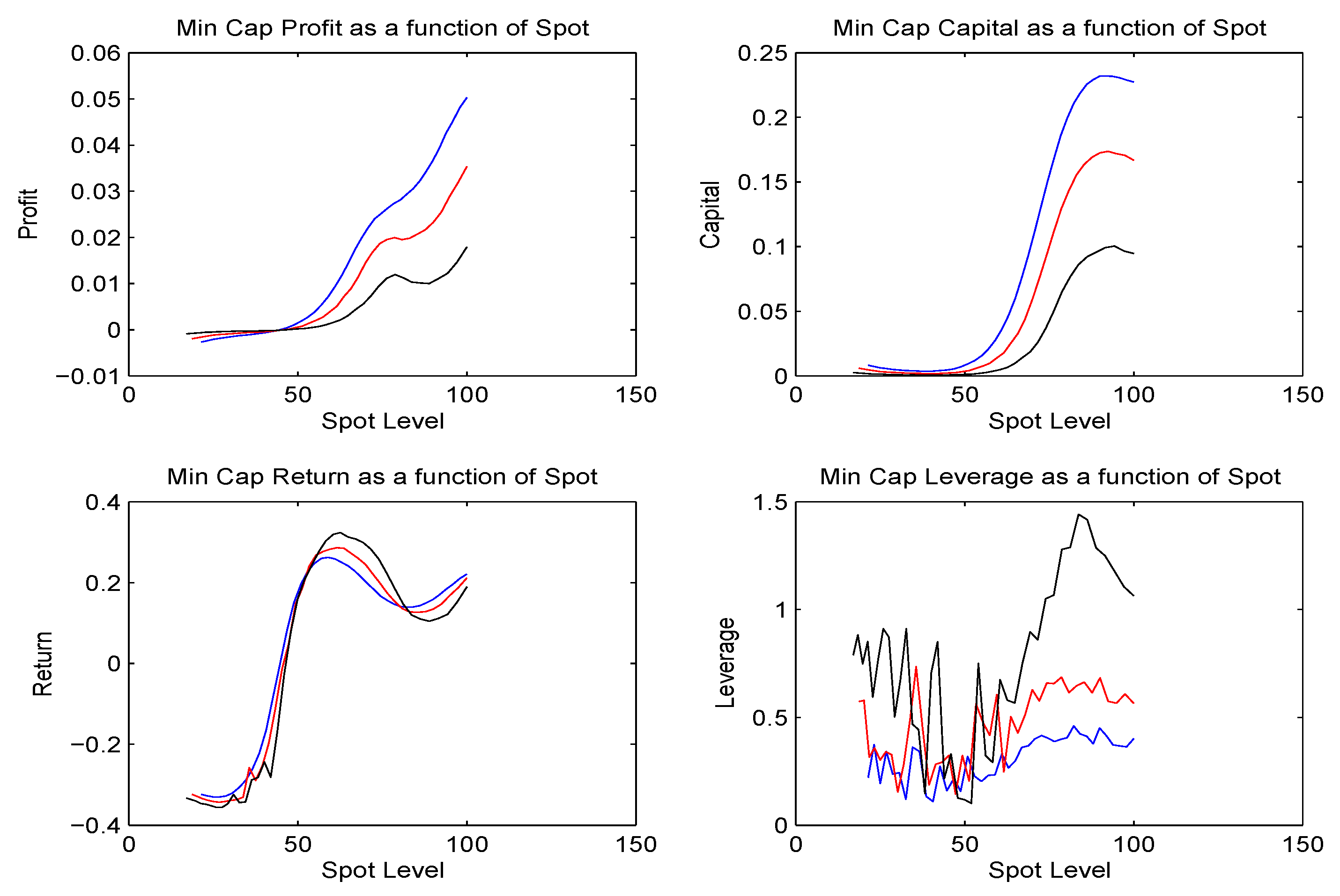
We present in Figure (4) and Figure (5) the profit, capital, return and leverage at 3, 6 and 9 months for the 120 one year Call and the 80 one year Put as functions of the level of the spot.
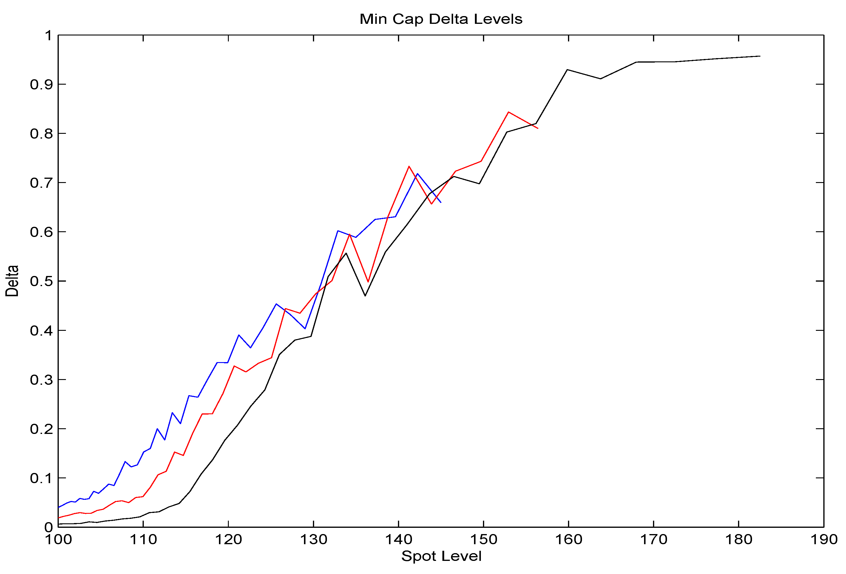
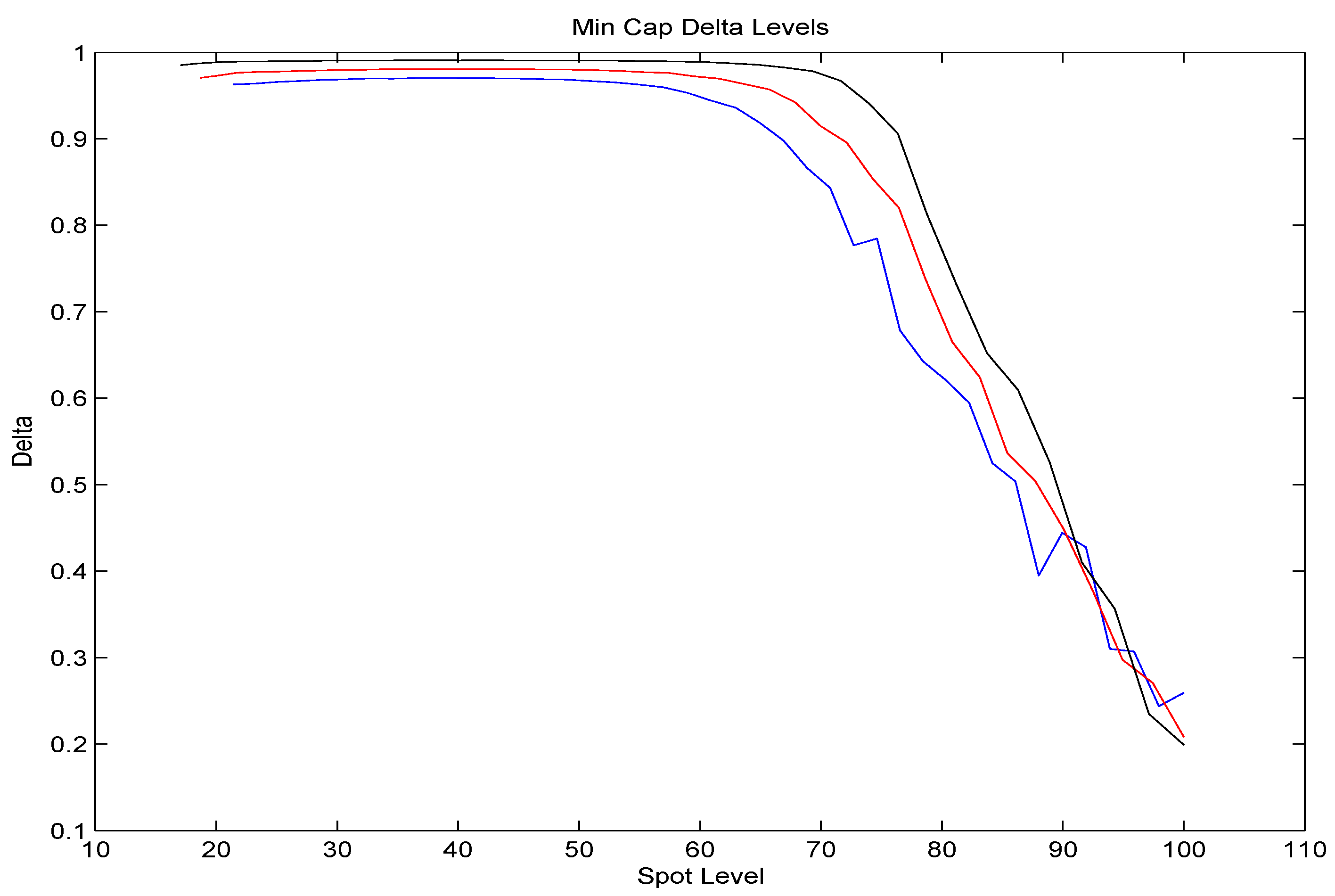
Additionally we present a graph for the delta positions taken in Figure (6) and Figure (7) to hedge the remaining risk with a view to minimizing reserve capital charges.
We also computed the dynamic levels of profit, capital, return and leverage for both the 120 one year call and 80 one year put using Black Scholes deltas computed at the implied volatility. The Black Scholes call deltas were considerably higher and the put deltas were lower in absolute value than what is observed under the optimal minimum capital hedge. We report in Table 3 the initial values for hedging at Black Scholes implied.
We observe that the capital levels are sufficiently higher for the Black Scholes delta hedge.
6 CONCLUSION
We present first in the static case and then in the dynamic case the argument for adjusting Black Scholes implied call deltas downwards for a gamma exposure in a left skewed market when the objective for the hedge is the conservation of capital. For similar reasons the absolute value of put deltas should be increased to accomodate the costs imposed on residual risks by the market skewness. The gamma adjustment factor in the static case is shown to be just a function of the risk neutral distribution that can be calibrated from the option surface. This could be periodically adjusted as skewness levels are observed to move around. In the dynamic case one may precompute at the date of trade initiation a matrix of delta levels as a function of the underlying for the life of the trade and subsequently one just has to look up the matrix for the hedge. Additionally the matrix could be periodically recalibrated. Also constructed are matrices for the capital reserve, the profit, leverage and rate of return remaining in the trade as a function of the spot at a future date in the life of the trade. These could be periodically recalibrated using the procedures outlined. The concepts of profit, capital, leverage and return are as described in Carr, Madan and Vicente Alvarez (2010).
The dynamic computations constitute an application of the theory of nonlinear expectations as described in Cohen and Elliott (2010) for a finite state stochastic difference equation framework. Bid and ask prices are computed as nonlinear expectations using a penalty driver for the periodic risk that comes from our static model. The dynamic implementation could be speeded up on employing the static adjustment factors as approximations where by one estimates gamma exposures by regression or the use of the Black Scholes gamma.
References
- P. Artzner, F. Delbaen, M. Eber, and D. Heath. “Coherent Measures of Risk.” Mathematical Finance 9 (1999): 203–228. [Google Scholar]
- P. Carr, D.B. Madan, and J.J. Vicente Alvarez. “Markets, Profits, Capital, Leverage and Return.” Working Paper, Robert H. Smith School of Business.
- A. Cherny. “Weighted VAR and its properties.” Finance and Stochastics, 2006, 10, 367–393. [Google Scholar]
- A. Cherny, and D.B. Madan. “Markets as a counterparty: An Introduction to Conic Finance.” International Journal of Theoretical and Applied Finance, 2010, 13, 1149–1177. [Google Scholar]
- A. Cherny, and D.B. Madan. “New Measures for Performance Evaluation.” Review of Financial Studies, 2009, 22, 2571–2606. [Google Scholar]
- P. Carr, H. Geman, and D.B. Madan. “Pricing and Hedging in Incomplete Markets.” Journal of Financial Economics 62 (2001): 131–167. [Google Scholar]
- A. Černý, and S. Hodges. “The Theory of Good Deal Pricing in Financial Markets.” In Mathematical Finance-Bachelier Congress 2000; Edited by H. D. Geman, S.R. Madan, Pliska and T. Vorst. Berlin: Springer, 2000. [Google Scholar]
- S. Cohen, and R.J. Elliott. “A General Theory of Finite State Backward Stochastic Difference Equations.” 2010, arXiv: 0810.4957v2. [Google Scholar]
- S. Cohen, and R.J. Elliott. “Comparisons for backward stochastic differential equations on Markov chains and related no-arbitrage conditions.” The Annals of Applied Probability 20 (2010b): 267–311. [Google Scholar]
- F. Delbaen, S. Peng, and E. Rosazza Gianin. “Representation of the penalty term of dynamic concave utilities.” Finance and Stochastics, 2010, 14, 449–472. [Google Scholar]
- N. El Karoui, and S.J. Huang. “Backward Stochastic Differential Equations, Pitman Research Notes in Mathematics, Longman.” 1997. [Google Scholar]
- S. Jaschke, and U. Küchler. “Coherent risk measures and good deal bounds.” Finance and Stochastics, 2001, 5, 181–200. [Google Scholar]
- A. Jobert, and L.C.G. Rogers. “Valuations and Dynamic Convex Risk Measures.” Mathematical Finance 18 (2008): 1–22. [Google Scholar]
- A. Jobert, and L.C.G. Rogers. “Valuations and Dynamic Convex Risk Measures.” Mathematical Finance 18 (2008): 1–22. [Google Scholar]
- D. Madan, P. Carr, and E. Chang. “The Variance Gamma Process and Option Pricing.” European Finance Review 2 (1998): 79–105. [Google Scholar]
- S. Kusuoka. “On Law Invariant Coherent Risk Measures.” Advances in Mathematical Economics 3 (2001): 83–95. [Google Scholar]
- D. Madan, and E. Seneta. “The variance gamma (V.G.) model for share market returns.” Journal of Business 63 (1990): 511–524. [Google Scholar]
- A. Mijatović, and M. Pistorius. “Continuously Monitored Barrier Options Under Markov Processes.” Working Paper. London: Imperial College. available at http://ssrn.com/abstract=1462822.
- S. Peng. “Dynamically consistent nonlinear evaluations and expectations.” Preprint No. 2004-1. Institute of Mathematics, Shandong University, 2004. available at http://arxiv.org/abs/math/0501415.
- E. Rosazza Gianin. “Risk Measures via g-expectations.” Insurance, Mathematics and Economics 39 (2006): 19–34. [Google Scholar]
Figure 1.
Capital as a function of the gamma adjustment factor

Figure 2.
120 one year Call Profits, Capital Return and Leverage as a function of the spot. At three months in blue, six months in red and 9 months in black.
Figure 2.
120 one year Call Profits, Capital Return and Leverage as a function of the spot. At three months in blue, six months in red and 9 months in black.
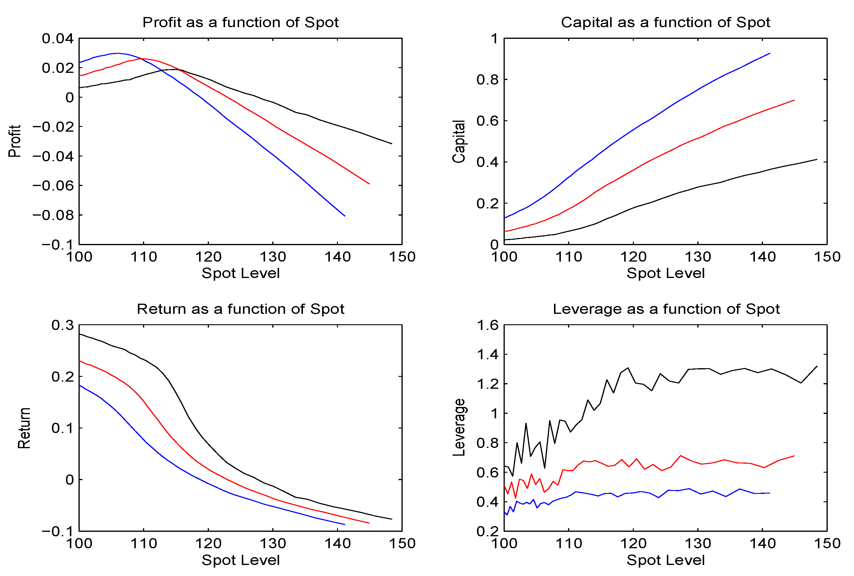
Figure 3.
80 one year put profit, capital, return and leverage as a function of the spot. At three months in blue, six months in red and 9 months in black.
Figure 3.
80 one year put profit, capital, return and leverage as a function of the spot. At three months in blue, six months in red and 9 months in black.
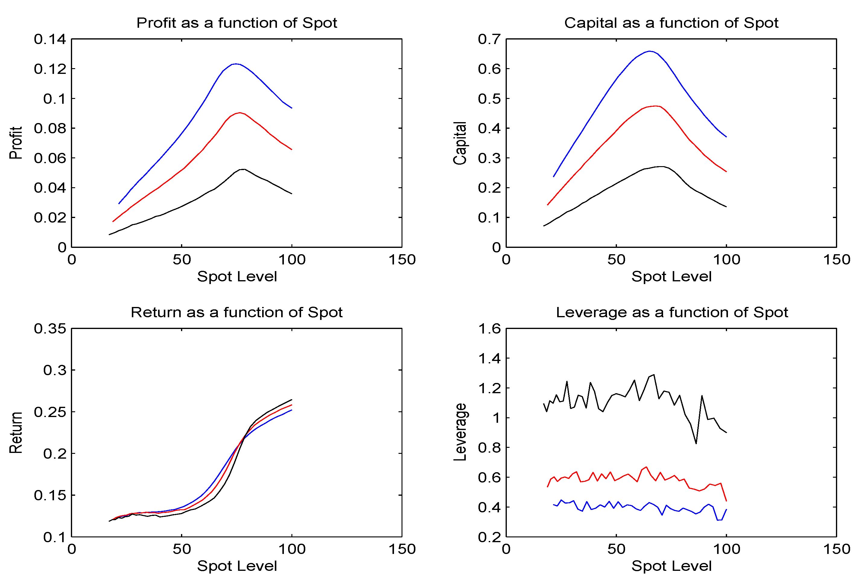
Figure 4.
Profit, Capital Return and Leverage with a minimum capital dynamic hedge as functions of the spot for a one year 120 call. At three months in blue, six months in red and nine months in black.
Figure 4.
Profit, Capital Return and Leverage with a minimum capital dynamic hedge as functions of the spot for a one year 120 call. At three months in blue, six months in red and nine months in black.
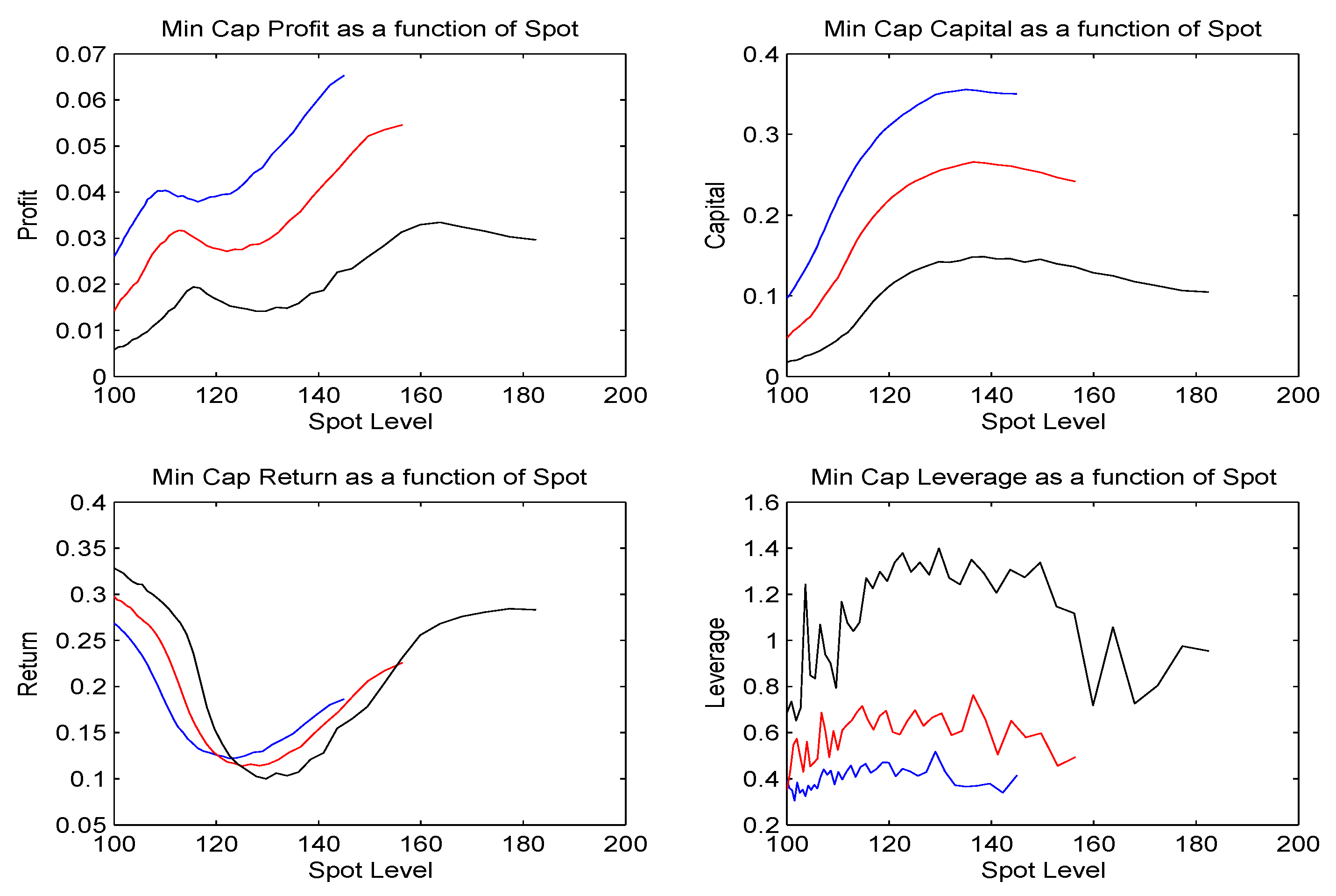
Figure 5.
Profit, Capital Return and Leverage with a minimum capital dynamic hedge as functions of the spot for a one year 80 put. At three months in blue, six months in red and nine months in black.
Figure 5.
Profit, Capital Return and Leverage with a minimum capital dynamic hedge as functions of the spot for a one year 80 put. At three months in blue, six months in red and nine months in black.

Figure 6.
Minimum capital delta positions as functions of the spot for the 120 one year call. At three months in blue, 6 months in red and 9 months in black.
Figure 6.
Minimum capital delta positions as functions of the spot for the 120 one year call. At three months in blue, 6 months in red and 9 months in black.

Figure 7.
Minimum capital delta positions as functions of the spot for the 80 one year put. At three months in blue, 6 months in red and 9 months in black.
Figure 7.
Minimum capital delta positions as functions of the spot for the 80 one year put. At three months in blue, 6 months in red and 9 months in black.


| bid | 5.0738 | 1.6162 |
| ask | 5.5572 | 1.8419 |
| mid | 5.3155 | 1.7291 |
| rne | 5.1966 | 1.6988 |
| scale | 0.1259 | 0.0670 |
| prf | 0.1189 | 0.0303 |
| cap | 0.4834 | 0.2256 |
| ret | 0.2460 | 0.1343 |
| bid | 4.6723 | 1.5221 |
| ask | 4.9465 | 1.6834 |
| mid | 4.8094 | 1.6028 |
| rne | 4.7471 | 1.5644 |
| scale | 0.0681 | 0.0476 |
| prf | 0.0623 | 0.0384 |
| cap | 0.2741 | 0.1613 |
| ret | 0.2273 | 0.2382 |
| bid | 3.8532 | 2.3318 |
| ask | 4.8601 | 3.8047 |
| mid | 4.3566 | 3.0683 |
| rne | 4.3386 | 2.9177 |
| scale | 0.1478 | 0.0904 |
| prf | 0.0180 | 0.1506 |
| cap | 1.0069 | 1.4728 |
| ret | 0.0179 | 0.1023 |
Share and Cite
MDPI and ACS Style
Madan, D.B. Conserving Capital by Adjusting Deltas for Gamma in the Presence of Skewness. J. Risk Financial Manag. 2010, 3, 1-25. https://doi.org/10.3390/jrfm3010001
AMA Style
Madan DB. Conserving Capital by Adjusting Deltas for Gamma in the Presence of Skewness. Journal of Risk and Financial Management. 2010; 3(1):1-25. https://doi.org/10.3390/jrfm3010001
Chicago/Turabian StyleMadan, Dilip B. 2010. "Conserving Capital by Adjusting Deltas for Gamma in the Presence of Skewness" Journal of Risk and Financial Management 3, no. 1: 1-25. https://doi.org/10.3390/jrfm3010001