Statistical Arbitrage with Mean-Reverting Overnight Price Gaps on High-Frequency Data of the S&P 500

Department of Statistics and Econometrics, University of Erlangen-Nürnberg, Lange Gasse 20, 90403 Nürnberg, Germany
*
Author to whom correspondence should be addressed.
J. Risk Financial Manag. 2019, 12(2), 51; https://doi.org/10.3390/jrfm12020051
Submission received: 27 February 2019
/
Revised: 24 March 2019
/
Accepted: 26 March 2019
/
Published: 1 April 2019
(This article belongs to the Special Issue Computational Finance)
Abstract
:This paper develops a fully-fledged statistical arbitrage strategy based on a mean-reverting jump–diffusion model and applies it to high-frequency data of the S&P 500 constituents from January 1998–December 2015. In particular, the established stock selection and trading framework identifies overnight price gaps based on an advanced jump test procedure and exploits temporary market anomalies during the first minutes of a trading day. The existence of the assumed mean-reverting property is confirmed by a preliminary analysis of the S&P 500 index; this characteristic is particularly significant 120 min after market opening. In the empirical back-testing study, the strategy delivers statistically- and economically-significant returns of 51.47 percent p.a.and an annualized Sharpe ratio of 2.38 after transaction costs. We benchmarked our trading algorithm against existing quantitative strategies from the same research area and found its performance superior in a multitude of risk-return characteristics. Finally, a deep dive analysis shows that our results are consistently profitable and robust against drawdowns, even in recent years.
1. Introduction
Statistical arbitrage is a market-neutral strategy developed by a quantitative group at Morgan Stanley in the mid-1980s (Pole 2011). Following Hogan et al. (2004), the self-financing strategy describes a long-term trading opportunity that exploits persistent capital market anomalies to draw positive expected profits with a Sharpe ratio that increases steadily over time. Arbitrage situations are identified with the aid of data-driven techniques ranging from plain vanilla approaches to state-of-the-art models. In the event of a temporary anomaly, an arbitrageur goes long in the undervalued stock and short in the overvalued stock (see Vidyamurthy (2004), Gatev et al. (2006)). If history repeats itself, prices converge to their long-term equilibrium and an investor makes a profit. Key contributions are provided by Vidyamurthy (2004), Gatev et al. (2006), Avellaneda and Lee (2010), Bertram (2010), Do and Faff (2012), and Chen et al. (2017).
The available literature divides statistical arbitrage into five sub-streams, including the time-series approach, which concentrates on mean-reverting price dynamics. Since financial data are exposed to more than one source of uncertainty, it is surprising that there exist only a few academic studies that use a jump-diffusion model (see Larsson et al. (2013), Göncü and Akyildirim (2016), Stübinger and Endres (2018), Endres and Stübinger (2019a,2019b)). In addition to mean-reversion, volatility clusters, and drifts, this general and flexible stochastic model is able to capture jumps and fat tails. First, Larsson et al. (2013) used jump-diffusion models to formulate an optimal stopping theory. Göncü and Akyildirim (2016) presented a stochastic model for the daily trading of commodity pairs in which the noise-term is driven by a Lévy process. Stübinger and Endres (2018) introduce a holistic pair selection and trading strategy based on a jump-diffusion model. Recently, Endres and Stübinger (2019a,2019b) derived an optimal pairs trading framework based on a flexible Lévy-driven Ornstein–Uhlenbeck process and applied it to high-frequency data. All these studies deal with intraday price dynamics and are therefore not in a position to take into account the impact of overnight price changes, an apparent deficit as information is published in media platforms 24 h a day, seven days a week.
This paper enhances the existing research in several aspects. First, our manuscript contributes to the literature by developing a fully-fledged statistical arbitrage framework based on a jump–diffusion model, which is able to capture intraday and overnight high-frequency price dynamics. Specifically, we detect overnight price gaps based on the jump test of Barndorff-Nielsen and Shephard (2004) and Andersen et al. (2010) and exploit temporary market anomalies during the first minutes of a trading day. The existence of the assumed mean-reverting property is confirmed by a preliminary analysis on the S&P 500 index; this characteristic is particularly significant 120 min after market opening. Second, the value-add of the proposed trading framework is evaluated by benchmarking it against well-known quantitative strategies in the same research area. In particular, we consider the naive S&P 500 buy-and-hold strategy, fixed threshold strategy, general volatility strategy, as well as reverting volatility strategy. Third, we perform a large-scale empirical study on the sophisticated back-testing framework of high-frequency data of the S&P 500 constituents from January 1998–December 2015. Our jump-based strategy produces statistically- and economically-significant returns of 51.47 percent p.a. appropriate after transaction costs. The results outperform the benchmarks ranging from −6.56 percent for the fixed threshold strategy to 38.85 percent for the reverting volatility strategy; complexity pays off. Fourth, a deep-dive analysis shows that our results are consistently profitable and robust against drawdowns even in the last part of our sample period, which is noteworthy as almost all statistical arbitrage strategies have suffered from negative returns in recent years (see Do and Faff (2010), Stübinger and Endres (2018)). The results pose a major challenge to the semi-strong form of market efficiency.
The remainder of this research study is structured as follows. Section 2 provides the theoretical framework applied in this study. In Section 3, we discuss the event study of the S&P 500 index. After describing the empirical back-testing framework in Section 4, we analyze our results and present key findings in Section 5. Finally, Section 6 gives final remarks and an outlook on future work.
2. Methodology
This section provides the theoretical construct of our statistical arbitrage strategy. Therefore, Section 2.1 describes the Barndorff–Nielsen and Shephard jump test (BNS jump test), which helps us to recognize jumps in our time series. The identification of overnight gaps is presented in Section 2.2.
2.1. Barndorff–Nielsen and Shephard Jump Test
We follow the theoretical framework of Barndorff-Nielsen and Shephard (2004) to detect overnight gaps. First, let us denote low-frequency returns as:
where denotes the log price of an asset after time interval and ℏ represents a fixed time period, e.g., trading days. These low-frequency returns can be split up into M equally-spaced high-frequency returns of the following form:
If i denotes the day, the intra-ℏ return is expressed as . Therefore, the daily return can be written as:
The BNS jump test of Barndorff-Nielsen and Shephard (2004) underlies the assumptions that prices follow a semi-martingale to ensure the condition of no-arbitrage and are generated by a jump-diffusion process of the following form and properties:
where describes the log price and represents the stochastic volatility semi-martingale process:
with describing the trend term with locally-finite variation paths, following a continuous mean process of the security. The stochastic volatility process is represented through , which is a local martingale and defined as:
where W describes the Wiener process. The spot volatility process is locally restricted away from zero and specified as càdlàg, meaning that the process is limited on the left side, while it is everywhere right continuous. Furthermore, , and the integrated variance () process:
satisfies . Moreover, defines the discontinuous jump component as:
with N representing a finite counting process, so that and denoting nonzero random variables. Putting all together, the process can be written as:
consisting of a stochastic volatility component that models continuous price motions and a jump term that accounts for sudden price shifts and discontinuous price changes. It is assumed that and are independent of W. From an economic point of view, Rombouts and Stentoft (2011) showed that neglecting the non-Gaussian features of the data, prices are estimated with large errors.
To conduct the BNS jump test, three volatility metrics need to be specified: The quadratic variation (), realized variance (), and bipower variation (). is defined as:
with denoting the integrated variance, presenting the quadratic variation of the continuous part of the semi-martingale process, while determines the quadratic variation of the jump component (see Andersen et al. (2001), Barndorff-Nielsen and Shephard (2002), Andersen et al. (2003), Barndorff-Nielsen and Shephard (2004), Barndorff-Nielsen and Shephard (2006)). Hence, this volatility measurement takes into account the total variation of the underlying jump-diffusion process.
The realized variance:
functions as a consistent estimator of , where M determines the number of intraday returns for day i. This volatility measure sums up all squared intraday returns for any considered period.
Andersen and Bollerslev (1998), Andersen et al. (2001), and Barndorff-Nielsen and Shephard (2002) showed that equals for large M, yielding to the equation:
was introduced by Barndorff-Nielsen and Shephard (2004) as:
where every periods of time observations exist in interval t. is a consistent estimator of under the assumption of a semi-martingale stochastic volatility process with a jump component described by Equation (4). Under those assumptions and for and applies:
where is a stochastic process, and is defined as:
with , u following a standard normal distribution, while denotes the complete gamma function.
Barndorff-Nielsen and Shephard (2004) focused on the special case of leading to the following equation:
Hence, is for a consistent estimator of the integrated volatility for the ith period. Based on this case, the variation of the jump term can be isolated by subtracting from :
By calculating the difference between and , we can separate the jump contribution to the variation of the asset price from the . Therefore, the volatility can be decomposed into its continuous and discontinuous components.
To identify jumps, we use the basic principles of the non-parametric BNS jump test and apply the ratio z-statistic from Huang and Tauchen (2005). This test statistic is adjusted for market noise and provides useful properties such as an appropriate size and a reasonable power. The evidence from the Monte Carlo simulation also suggests that this z-test is fairly accurate in detecting real jumps and not easily fooled by market micro structure noises. The ratio test statistic:
is asymptotic standard normally distributed under the null hypothesis of no jumps. Following Huang and Tauchen (2005), the tripower quarticity statistic is calculated by the following equation:
To determine if at least one jump occurred in an asset, a right-sided hypothesis test with the null hypothesis of no jumps was conducted. A commonly-used level of significance is 0.1 percent (see Barndorff-Nielsen and Shephard (2006), Evans (2011), Frömmel et al. (2015)). If the null hypothesis was rejected, at least one jump emerged in the underlying security during the considered period.
2.2. Jump Detection Scheme
The timing of jumps has an essential meaning for examining anomalous behavior around jumps. To identify overnight gaps via jump tests, the precise time must be known. For this purpose, we rely on the jump detection scheme introduced by Andersen et al. (2010). This jump identification procedure is designed on the premise that jumps are rare events. If it is assumed that t equals one day and at most one jump can emerge during the corresponding period, the only intraday jump can be determined with:
where represents the jump variation in period t. The intuitive idea is that the jump must be incorporated in the highest absolute return on that specific day. Hence, the timing of the jump can be determined by seeking the highest absolute return of the period. Furthermore, the precise jump size can be calculated in the following way:
where denotes the intraday return that contains the jump contribution, while is equal to 1 or , depending on the sign of the argument.
3. Event Study of the S&P 500 Index
This section uses the outlined methodology of Section 2 to identify and analyze overnight price gaps in the S&P 500 index. Following the approaches of Fung et al. (2000) and Grant et al. (2005), we conducted the following four steps.
At first, the data were filtered according to the event of interest, the presence of overnight gaps. To identify overnight gaps, we conducted daily the BNS jump tests, as introduced in Section 2.1. For the test, we used high-frequency intraday returns of the previous day and the overnight return and a significance level of 0.1 percent. The timing of jumps was determined by the jump detection procedure of Andersen et al. (2010) (see Section 2.2). If the timing of the jump corresponded with the overnight return, the day was marked as an event day and included in our study.
Second, for every event day, the cumulative return of the S&P 500 index at minute t after the market opening was computed by:
where denotes the index price on event day i at minute t after the beginning of the trading day. Respectively, represents the market opening.
Third, the average cumulative return () at time t:
was computed for all event days. This figure is available for any minute t after the start of the trading day. N is defined as the total number of days fulfilling the event day properties.
Fourth, t-tests were conducted to determine whether a given price movement after a specified event was significant. Specifically, we calculated the corresponding test statistic to examine if the at time t was significantly distinct from zero. The test statistic had the following form:
where and denotes the mean of the sample. Furthermore, represents its standard deviation, and N defines the total numbers of days in the filtered dataset. Under the null hypothesis of no distinction from zero, the test statistic follows a t-distribution with degrees of freedom.
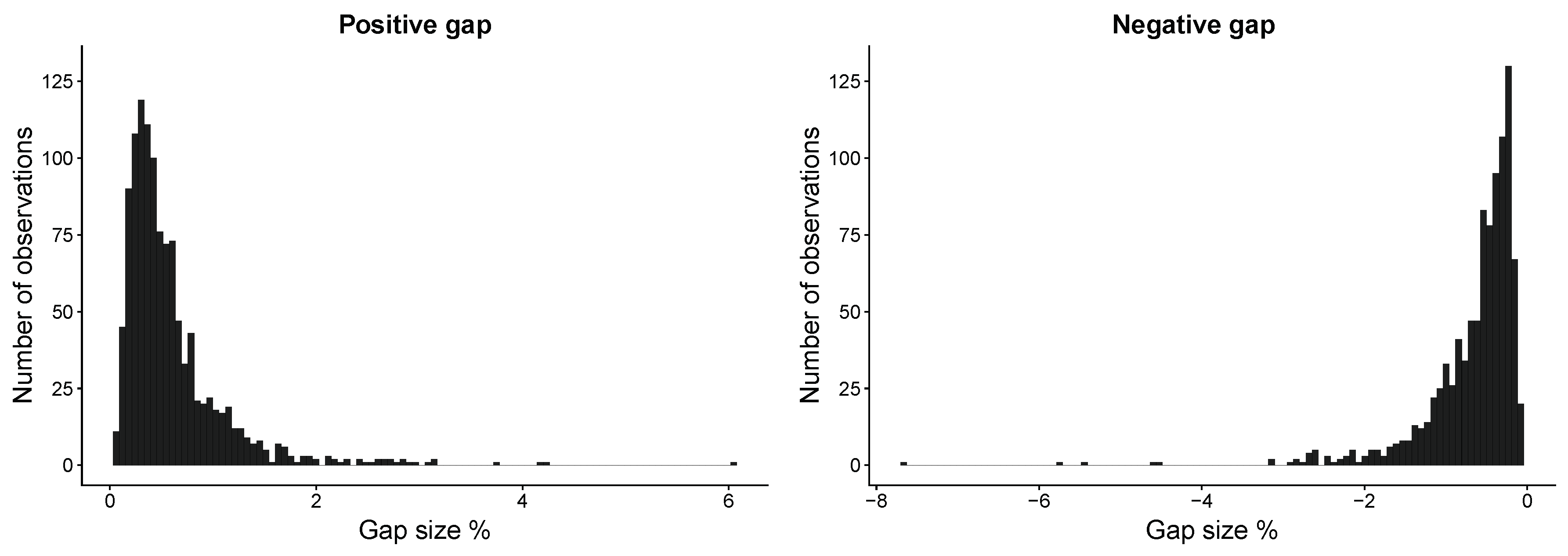
Table 1 shows the characteristics of the overnight price gaps detected by our jump test procedure. In total, we observed 2128 overnight gaps during the sample period: 1154 of those gaps were positive, while 974 were negative. On average, the S&P 500 index faced positive (negative) overnight gaps of 0.60 percent (−0.67 percent). The largest overnight gaps occurred during the global financial crisis with 6.02 percent and −7.64 percent. The fact that both the range and the standard deviation of negative gaps were higher than those of positive overnight movements confirms the existing literature: market participants tend to react stronger to bad news rather than to good headlines (Suleman 2012). Concluding, Table 1 shows that there was a sufficient number of overnight price gaps leading to temporary market inefficiencies. As a result, this jump behavior generated high-frequency stock price dynamics that created major trading opportunities. In stark contrast to the approach of Fung et al. (2000) and Grant et al. (2005), the gaps identified by our jump-test scheme were both flexible and data-driven.
Figure 1 illustrates the detected jumps in a more detailed way. We observe a higher variation of negative overnight gaps, which is not surprising since financial data possess an asymmetric distribution (Cont 2001). Interestingly, the interval with the highest number of observations for both positive and negative overnight gaps was about .
Figure 2 presents the number of detected overnight gaps over time. With rising volatility in financial markets, the number of overnight gaps also increased; fluctuations in the market imply jumps. Thus, it is not surprising that we observed almost no jumps in the first years of our sample period. In stark contrast, the number of overnight price gaps increased in times of high market turmoil. In general, more positive than negative gaps affect the S&P 500 index. As expected, this pattern changes during crises such as the dot-com crash in the early 2000s and the financial crisis in 2008. This also demonstrates the flexibility of the approach used to identify overnight gaps.
Figure 3 depicts the average cumulative returns after overnight gaps identified by the BNS jump test. The detailed development of the for positive and negative price gaps is reported in Table A1. The typical price pattern after overnight gaps is still persistent in modern financial markets, despite that markets should become more efficient in the course of digitalization and improved information flow (see Fung et al. (2000) and Grant et al. (2005)). In the case of a positive overnight gap, the average cumulative returns rose for a brief period before reverting to the minimum at −0.0316 percent. After reaching the lowest 105 min after market opening, it began to rise until it crossed the zero percent line. From this point, the returns almost fell close to the minimum before increasing again. The upswing accelerated towards market closing, reaching 0.0236 percent at the end of the trading day. Following a negative overnight gap, the move inverted. Starting with a brief continuation of the initial overnight movement, which marked the minimum of −0.0093 percent two minutes after the stock exchange opens, the began to reverse to its maximum of 0.0463 percent after approximately one and a half hours. The remained relatively stable between 0.0200 and 0.0400 percent subsequent to hitting the upper limit. During the last ten minutes, the rapidly decreased until the end of the trading day. Noticeable is that the magnitude of the variation of the was stronger after negative price gaps. This is in line with stronger expected reactions of market participants to bad information that was also observable in the represented gap characteristics (Table 1). The p-values for both realizations indicated that the returns were statistically different from zero on a 10 percent significance level for most of the time before the 115-min mark. After that threshold has passed, p-values well exceeded 10 percent; this fact is not surprising since many professional day traders stop trading after two trading hours because volatility and volume tend to decrease (see Balance (2019)). Furthermore, we recognized that the for positive overnight gaps were not significant for a target time of 5, 35, 65, and 95 min based on a 10% significance level; it seems that the pattern is systematically repeated at 30-min intervals. This statement is confirmed by Business Insider (2015), which shows that the trading volume increases in the first minutes of every trading hour. Furthermore, Bedowska-Sojka (2013) demonstrated that this volatility is influenced by macroeconomic releases, which are typically published at 9:30, 10:00, 10:30, and 11:00. As a result, the test-statistic decreased, leading to non-significant p-values.
Concluding, our event study confirms the overreaction hypothesis and supports the results of Fung et al. (2000) and Grant et al. (2005). The findings of the event study further suggest that we are in a position to develop a statistical arbitrage strategy that exploits the mean-reversion characteristic of stocks after statistically-significant overnight price gaps (see Poterba and Summers (1988), Leung and Li (2015), Lubnau and Todorova (2015)). Specifically, it seems profitable to open trades after overnight gaps and close them after 2 h, i.e., we should set a target time of 120 min.
4. Back-Testing Framework
The empirical back-testing study was performed from January 1998–December 2015 at intraday prices for the S&P 500 index components (see Section 4.1). According to Gatev et al. (2006) and Nakajima (2019), we divided the dataset into overlapping study periods, which were shifted by one day each. Each study period consisted of two consecutive phases. In the formation period (Section 4.2), the most appropriate stocks were selected using predefined models and criteria. In the subsequent out-of-sample trading period (Section 4.3), the top stocks were traded using rule-based entry and exit signals; this procedure avoids any look-ahead bias. Summarizing, we developed a full-fledged statistical arbitrage framework based on a jump–diffusion model (JDS), which is able to capture intraday and overnight high-frequency price dynamics.
4.1. Data and Software
The empirical back-testing was based on intraday data from the S&P 500 from January 1998–December 2015. This highly liquid stock market includes the stocks of the 500 leading blue chip companies that offer high-quality commodities and generally-accepted services. Since the S&P 500 index captures 80 percent of the total U.S. market capitalization (S&P Dow Jones Indices 2015), this dataset represents a fundamental test for any potential capital market anomaly. To be in line with Stübinger and Endres (2018), we applied a two-step process with the objective of removing any survivor bias from the database. First, we used the information list from QuantQuote (2016) to build a binary constituent matrix for S&P 500 shares from January 1998–December 2015. The 4527 rows characterize the trading days considered, and the 984 columns show the stocks that were ever in the S&P 500. Each element of this matrix displays a “1” if the corresponding company is part of the S&P 500 index on the corresponding day, otherwise a “0”. The sum of each row is about 500 because on each trading day, there are approximately 500 stocks in the index. Second, the complete archive of minute-by-minute prices from January 1998–December 2015 was downloaded from QuantQuote (2016). The corresponding stock exchange was open from Monday to Friday from 9:30–16:00 Eastern time. Consequently, the price time series of a share includes 391 data points per day. We followed Stübinger and Endres (2018) and adjusted the data by stock splits, dividends, and other corporate actions. By performing these two steps, our study design is in a position to map the constituents of the S&P 500 and the corresponding price time series completely.
The presented methodology and all relevant evaluations were implemented in the statistical programming language R (R Core Team 2019). For computation-intensive calculations, we used both the general-purpose programming language C++ and on-demand cloud computing platforms with virtual computer clusters that are available 24/7 via the Internet.
4.2. Formation Period
In the formation period, we considered all S&P 500 stock constituents. Therefore, we (i) conducted the BNS jump test based on past returns (ii) applied the jump detection scheme in the case of rejecting the null hypothesis, and (iii) selected the top stocks for the subsequent trading period. This subsection describes the outlined three-step logic.
In the first step, we executed the BNS jump test based on both the 390 intraday returns of the last trading day and the overnight return, i.e., the percentage change of the price from 16:00 of the last day to 9:30 of the current trading day. Specifically, we determined the z-statistic of Huang and Tauchen (2005) (see Equation (18)). If the null hypothesis was rejected, at least one jump emerged in the underlying security during the considered period. If the null hypothesis was not rejected, no jump emerged in the underlying security during the considered period. Consequently, we did not consider this stock in our back-testing framework.
In the second step, we applied the jump identification method of Andersen et al. (2010) to ensure that we only selected stocks possessing overnight gaps (see Section 2.2). Therefore, we considered only stocks that incorporate a significant overnight gap.
In the third step, we followed Miao (2014) and Stübinger and Endres (2018) and selected the most suitable shares for the out-of-sample trading period. Our algorithm attempted to find stocks possessing the most meaningful jump last night. For this purpose, we selected the top stocks, that possesses overnight gaps in the sense of Andersen et al. (2010), with the highest z-statistic of Huang and Tauchen (2005). The top 10 stocks were transferred to the trading period (see Section 4.3)1.
4.3. Trading Period
The top 10 stocks with the highest z-statistic were considered in the one-day trading period. For every top stock, we applied the following trading rules:
- We observe a negative price gap during the night, i.e., the stock is undervalued. Consequently, we go long in the stock.
- We observe a positive price gap during the night, i.e., the stock is overvalued. Consequently, we go short in the stock.
Motivated by Section 3, the trade was reversed 120 min later. Our strategy was based on a two-stage logic. First, we identified significant overnight price changes that had a substantial impact on future stock prices. Second, the top stocks possessed mean-reverting price dynamics, so that we could take advantage of these temporary market inefficiencies. If our assumption was correct, we were in a position to capture transient mispricings and generate profits. Concluding, we created a statistical arbitrage strategy based on a mean-reverting jump-diffusion model, the individual jump threshold depends on the underlying volatility.
As we aim for a classic long-short investment strategy in the sense of Gatev et al. (2006), we followed the principles of Avellaneda and Lee (2010) and Stübinger et al. (2018) and secured the market exposure with appropriate capital investments in the S&P 500 index. Every activity carried out on the market involves transaction costs. Therefore, it would be naive to ignore these fees as our high-frequency framework is based on permanent trading. According to Prager et al. (2012) and Stübinger and Bredthauer (2017), estimating exact values is not possible, but the bid-ask spread had abated to lower than one percent for stocks of the S&P 500 index, i.e., two basis points for an average stock price of 50 USD. In the same vein, Voya Investment Management (2016) accounted for a bid-ask spread of 3.5 basis points for the S&P 500, which was caused by increased use of algorithmic trading, decimalization, and changes in the stock market landscape. To be in line with Stübinger and Endres (2018), we assumed transaction costs of five basis points per share per half-turn. Consequently, transaction costs per complete round-trip corresponded to 20 basis points. This assumption appears realistic in light of our high-turnover strategy in a highly-liquid equity market.
In order to evaluate the value-add of our strategy, we benchmarked it against strategies from the same research field, but less flexible. More specifically, we considered the S&P 500 buy-and-hold strategy (BHS), fixed threshold strategy (FTS), general volatility strategy (GVS), and reverting volatility strategy (RVS) (see Table 2). The characteristic “individual” implies that the trading behavior depends on the underlying variable. If the model captured the behavior of fluctuations of stock price dynamics, we assigned the “volatility” property. The feature “mean-reverting” was fulfilled for statistical approaches that were able to model convergence to equilibrium after divergence. Finally, the explicit inclusion of a jump term led to the characteristic “jump-diffusion”. Data and the general frame were set identically to the JDS in order to ensure a fair comparison. Especially, we transferred the top 10 stocks to the trading period for each day across all strategies. Details of the four benchmark strategies are presented in the following paragraphs.
S&P 500 Buy-and-Hold Strategy (BHS)
First, we compared JDS to a naive S&P 500 buy-and-hold strategy (BHS). To be more specific, the index was bought in January 1998 and held during the complete time period. This passive investment neglected all the characteristics required for a successful strategy, namely, “individual”, “volatility”, “mean-reverting”, and “jump-diffusion”.
Fixed Threshold Strategy (FTS)
According to Fung et al. (2000), Grant et al. (2005), and Caporale and Plastun (2017), the fixed threshold strategy (FTS) detects abnormal overnight changes using a fixed threshold of percent. This benchmark strategy obtains an individual trading limit for each stock. In our framework, the top 10 stocks with the highest absolute changes were opened at 9:30 of the trading day. We went long in the undervalued stocks and went short in the overvalued stocks. Identical to JDS, the positions were reversed 120 min after market opening. This approach was not in a position to distinguish stocks on the basis of their fluctuation behavior.
General Volatility Strategy (GVS)
The general volatility strategy (GVS) is based on the assumption that equities with high volatility exhibit temporary market inefficiencies (see Banerjee et al. (2007), Bariviera (2017)). Following Stübinger and Endres (2018), we calculated the standard deviation of the overnight returns of the last 40 days and transferred the top 10 stocks with the highest volatility to the trading period. Again, undervalued (overvalued) stocks were bought (sold), and trades were reversed after 120 min.
Reverting Volatility Strategy (RVS)
Last but not least, the reverting volatility strategy (RVS) adds the mean-reversion component to GVS, i.e., we measured the degree of reversion to the equilibrium level after divergences. According to Do and Faff (2010), we determined the mean-reversion speed by the number of zero-crossings, which is defined as the number of times prices cross the zero line. Stocks were ranked separately by standard deviation and zero crossings; the stock with the highest value was assigned the highest rank for each measurement. Next, we formed a combined rank by the sum of the two separate ranks. The top 10 stocks were received by selecting stocks with the highest overall rank. The main disadvantage of this approach was the lack of a jump term, which reflects uncertainty in addition to the volatility component (Cartea et al. 2015).
5. Results
Following the high-frequency research studies of Mitchell (2010) and Knoll et al. (2018), we conducted a fully-fledged performance evaluation for the top 10 stocks of JDS from January 1998–December 2015 compared to the benchmarks BHS, FTS, GVS, and RVS. In particular, we evaluated the return characteristics and risk metrics (Section 5.1), examined the performance over time (Section 5.2), and analyzed the robustness of the strategies (Section 5.3). According to Gatev et al. (2006) and Avellaneda and Lee (2010), this paper calculated the total return based on committed capital, i.e., we divided the sum of daily net profits at the current day by the deployed capital.
5.1. Risk-Return Characteristics
Table 3 shows the daily return characteristics and risk metrics before and after transaction costs for the top 10 stocks per strategy from January 1998–December 2015. We observed statistically-significant returns for FTS, GVS, RVS, and JDS with Newey–West (NW) t-statistics above 15 prior to transaction costs. From an economical point of view, daily returns ranged between 0.17 percent for FTS and 0.36 percent for JDS. If we considered transaction costs, only the mean-reverting strategies RVS and JDS produced positively significant daily returns of 0.13 percent (RVS) and 0.17 percent (JDS). As expected, BHS generated statistically non-significant returns of 0.02 percent per day (see Endres and Stübinger (2019b)). The range, i.e., the difference of the maximum and minimum, was vastly different for JDS (approximately 0.30 percentage points), compared to BHS, FTS, GVS, and RVS (approximately 0.15 percentage points); this dissimilarity is potentially driven by the jump-diffusion term. The same argument explains the increased standard deviation of JDS. All individual strategy variants depicted favorable characteristics for any potential investor due to the fact that the underlying returns showed right skewness and followed a leptokurtic distribution (Cont 2001). We found that the maximum drawdown was quite different for FTS (87.84 percent) and GVS (89.47 percent), in contrast to RVS (55.91 percent), BHS (64.33 percent), and JDS (68.17 percent); the difference between non-reverting and reverting top stocks is clearly pointed out. The hit rate of JDS, i.e., the percentage of days with non-negative returns, outperformed with 58.41 percent after transactions costs, compared to the benchmarks, ranging between 41.79 percent for FTS and 55.92 percent for RVS.
In Table 4, we depict annualized risk-return measures before transaction costs (left side) and after transaction costs (right side). After transaction costs, JDS produced returns of 51.47 percent p.a., compared to 38.85 percent for RVS, −4.07 percent for GVS, and −6.59 percent for FTS. Thus, the first two strategies achieved meaningfully better results than the naive buy-and-hold strategy (BHS) with an average return of 1.81 percent p.a. Across all strategies, the mean excess return was similar to the mean return because the risk-free rate was very close to zero, especially in the last years. Our jump-based strategy JDS generated approximately the standard deviation of the market, resulting in a Sharpe ratio of 2.38 after transaction costs. This value confirmed the results of the high-frequency studies of Knoll et al. (2018) and Stübinger (2018). The lower partial moment risk of JDS led to a Sortino ratio of 4.76, compared to the benchmarks ranging between −1.03 (FTS) and 4.67 (RVS). We summarized that JDS outperformed the classic approaches in a large number of comparisons; complexity pays off. Our task was still to evaluate the performance over time, as well as the robustness of the strategies.
5.2. Sub-Period Analysis
Motivated by the time-varying returns of Liu et al. (2017) and Stübinger and Knoll (2018), we analyzed the stability and potential of the strategies over time. Figure 4, therefore, presents the development of an investment of USD 1 after transaction costs for FTS, GVS, RVS, JDS (first column), and the S&P 500 buy-and-hold strategy BHS (second column) over three partial periods. Table A2 provides a detailed overview of the corresponding annualized risk-return ratios for sub-periods of three years.
The first sub-period ran from 1998–2006 and described the bursting of the Internet bubble and the start of the Iraq war, as well as the subsequent bull market. We observed meaningful differences in performance between the mean-reverting and non-mean-reverting strategies: the average annual returns after transaction costs of up to 73.76 percent for RVS and up to 64.08 percent for JDS were well above those of BHS (7.87 percent), FTS (27.31 percent), and GVS (42.26 percent). As a typical feature in the financial context, the baseline methods were nevertheless successful in this period due to market inefficiencies and a lack of transparency.
The second sub-period ranged from 2007–2009 and was characterized by the global financial crisis and its consequences. In the course of the sub-prime crisis, the overall market showed strong fluctuations and substantial declines. In contrast, the other strategies generated positive returns, ranging from 27.35 percent for FTS to 315.02 percent for JDS. This strong performance was not astonishing as Avellaneda and Lee (2010) and Rad et al. (2016) demonstrated that statistical arbitrage trading strategies achieved abnormal returns during bear markets.
The third sub-period extends from 2010–2015 and covered a period of comebacks and restarts. The benchmarks FTS and GVS showed declining trends compared to the overall market, caused by the increasing public availability of these methods. RVS achieved an almost constant cumulative return of one, i.e., this strategy generated exactly the costs that were incurred. For JDS, we observed that 1 USD invested in January 2010 grew to 5 USD after transaction costs; performance did not decline across time and seemed to be robust against drawdowns.
5.3. Robustness Check
As mentioned above, we motivated the target time of 120 min based both on the available literature and the results of our event study; see Section 3. Since data snooping is a major problem in many financial applications, this subsection examines the sensitivity of our strategies to deviations from their parameter value. In Table 5, we vary the target time in two directions and report the annualized returns before and after transaction costs for BHS, FTS, GVS, RVS, and JDS.
First of all, we see that our results were robust in the face of parameter variations and always led to statements similar to those in Section 5.1. As expected, the results of a target time of 120 were identical to those of Table 3. Furthermore, the annualized returns for each strategy converged as the relative change decreased with increasing target time. The naive S&P 500 buy-and-hold strategy (BHS) always led to an annualized return of 1.81 percent, which is not surprising, since this approach is completely independent of the target time (Section 4). Furthermore, the performance of FTS increased slightly with ascending target time, e.g., the annualized return after transaction costs was −9.37 percent if we closed the trade at 9:50 and −8.36 percent if we closed it at 13:10. The same statement applies to GVS (−9.70 percent vs. −4.28 percent). Due to their mean-reverting component, RVS and JDS showed a slightly declining performance. For each target time, JDS remained the best variant with annualized returns between 49.65 percent and 62.61 percent, after transaction costs. Obviously, we were not on an optimum, but we found robust trading results, regardless of fluctuations in our parameter setting.
Motivated by the findings in Section 3, Table 6 examines the annualized returns for a target time of 5, 35, 65, and 95 min. Most interestingly, annual returns were substantially lower for a target time of 5 min for FTS, GVS, RVS, and JDS because high market turmoil during the opening minutes reduced the results. For a target time of 35, 65, and 95 min, increasing market efficiency during the first minutes of each trading hour did not affect yearly returns before and after transaction costs; our strategies seem to be robust against this effect.
Next, we take a closer look at our S&P 500 buy-and-hold strategy (BHS). The S&P 500 index was purchased in January 1998 and was held for the entire sample period. Of course, BHS is only a baseline approach for betting on the market. Therefore, we followed Endres and Stübinger (2019b) and developed a more realistic benchmark: The S&P 500 strategy buys the index at 9:30 and reverses it after 120 min. We observed an annualized return of 1.03% compared to 1.81% for BHS (see also Table 4). This insufficient performance is not surprising, as it is a baseline approach without modeling.
Finally, this manuscript supposed a high-turnover strategy of an institutional trader on high-frequency prices. Motivated by the literature, our back-testing framework assumed transaction costs of five basis points per share per half-turn, resulting in 20 basis points per round-trip per pair. However, other traders may be less aggressive in implementing this strategy. Therefore, we analyzed the breakeven point of the statistical arbitrage strategy since investors are exposed to different market conditions. We found that the breakeven point of JDS was between 35 basis points and 40 basis points. Concluding, this strategy generated promising results, even for investors that are exposed to different market conditions and thus higher transaction costs.
6. Conclusions
In this paper, we presented an integrated statistical arbitrage strategy based on overnight price gaps and implemented it on high-frequency data of the S&P 500 stocks from January 1998–December 2015. In this context, we made four contributions to the literature. The first contribution relates to the developed trading framework based on a jump-diffusion model: we are in a position to capture jumps, mean-reversion, volatility clusters, and drifts. Our approach identifies overnight price gaps based on the jump test of Barndorff-Nielsen and Shephard (2004) and exploits temporary market anomalies by corresponding investments. In a preliminary study, we confirmed the assumption of mean-reverting overnight gaps with the aid of the S&P 500 index. The second contribution focuses on the value-add of our strategy. Therefore, we benchmarked it against well-known quantitative strategies from the same research area, namely the naive S&P 500 buy-and-hold strategy, fixed threshold strategy, general volatility strategy, and reverting volatility strategy. The third contribution is based on our large-scale empirical study on a sophisticated back-testing framework. Our strategy produced statistically- and economically-significant returns of 51.47 percent p.a. after transaction costs; the benchmarks were outperformed. The fourth contribution focuses on the profitable and robust performance results also in the last part of our sample period. Our findings posited a severe challenge to the semi-strong form of market efficiency even in recent times.
We identified three possible directions for further research: First, the event study and the back-testing framework should be conducted in other equity universes. Second, the exit signal of the strategy should be determined for each stock individually. Third, a multivariate model could be developed that takes into account the common interactions between stocks.
Author Contributions
J.S. and L.S. conceived of the research method. The experiments were designed by J.S. and performed by L.S. The analyses were conducted and reviewed by J.S. and L.S. The paper was initially drafted by J.S. and revised by L.S. It was refined and finalized by L.S. and J.S.
Funding
We are grateful to the “Open Access Publikationsfonds”, which has covered 75 percent of the publication fees.
Acknowledgments
We are further grateful to Ingo Klein and two anonymous referees for many helpful discussions and suggestions on this topic.
Conflicts of Interest
The authors declare no conflict of interest.
Appendix A

Table A1.
Detailed development of the with p-values of the two-sided t-test from January 1998–December 2015. denotes the average cumulative returns.
Table A1.
Detailed development of the with p-values of the two-sided t-test from January 1998–December 2015. denotes the average cumulative returns.
| Positive Gap | Negative Gap | |||
|---|---|---|---|---|
| Target Time | in % | -Value | in % | -Value |
| 5 min | 0.0056 | 0.1180 | 0.0013 | 0.8140 |
| 10 min | −0.0037 | 0.4690 | 0.0178 | 0.0180 |
| 15 min | −0.0155 | 0.0160 | 0.0334 | 0.0000 |
| 20 min | −0.0229 | 0.0020 | 0.0293 | 0.0060 |
| 25 min | −0.0248 | 0.0030 | 0.0355 | 0.0030 |
| 30 min | −0.0207 | 0.0260 | 0.0310 | 0.0160 |
| 35 min | −0.0150 | 0.1580 | 0.0327 | 0.0320 |
| 40 min | −0.0193 | 0.0850 | 0.0284 | 0.0670 |
| 45 min | −0.0245 | 0.0400 | 0.0314 | 0.0480 |
| 50 min | −0.0227 | 0.0670 | 0.0318 | 0.0560 |
| 55 min | −0.0236 | 0.0610 | 0.0415 | 0.0160 |
| 60 min | −0.0255 | 0.0490 | 0.0420 | 0.0150 |
| 65 min | −0.0209 | 0.1230 | 0.0346 | 0.0490 |
| 70 min | −0.0231 | 0.1000 | 0.0333 | 0.0690 |
| 75 min | −0.0257 | 0.0810 | 0.0387 | 0.0470 |
| 80 min | −0.0287 | 0.0600 | 0.0417 | 0.0310 |
| 85 min | −0.0301 | 0.0490 | 0.0432 | 0.0280 |
| 90 min | −0.0256 | 0.1030 | 0.0415 | 0.0360 |
| 95 min | −0.0230 | 0.1540 | 0.0373 | 0.0690 |
| 100 min | −0.0286 | 0.0810 | 0.0338 | 0.0990 |
| 105 min | −0.0316 | 0.0550 | 0.0334 | 0.1060 |
| 110 min | −0.0288 | 0.0820 | 0.0334 | 0.1070 |
| 115 min | −0.0294 | 0.0780 | 0.0382 | 0.0740 |
| 120 min | −0.0248 | 0.1360 | 0.0328 | 0.1260 |
| 130 min | −0.0189 | 0.2620 | 0.0307 | 0.1670 |
| 140 min | −0.0207 | 0.2290 | 0.0256 | 0.2660 |
| 150 min | −0.0224 | 0.2150 | 0.0343 | 0.1430 |
| 160 min | −0.0177 | 0.3300 | 0.0313 | 0.1920 |
| 170 min | −0.0156 | 0.3940 | 0.0295 | 0.2230 |
| 180 min | −0.0091 | 0.6250 | 0.0248 | 0.3160 |
| 190 min | −0.0066 | 0.7270 | 0.0276 | 0.2620 |
| 200 min | −0.0069 | 0.7180 | 0.0296 | 0.2320 |
| 210 min | −0.0111 | 0.5700 | 0.0340 | 0.1770 |
| 220 min | −0.0070 | 0.7210 | 0.0304 | 0.2370 |
| 230 min | −0.0027 | 0.8880 | 0.0258 | 0.3260 |
| 240 min | −0.0038 | 0.8450 | 0.0288 | 0.2650 |
| 250 min | −0.0068 | 0.7300 | 0.0254 | 0.3340 |
| 260 min | −0.0121 | 0.5460 | 0.0302 | 0.2640 |
| 270 min | −0.0175 | 0.3850 | 0.0314 | 0.2470 |
| 280 min | −0.0218 | 0.2890 | 0.0275 | 0.3260 |
| 290 min | −0.0212 | 0.3130 | 0.0241 | 0.3960 |
| 310 min | −0.0189 | 0.3880 | 0.0347 | 0.2390 |
| 330 min | −0.0131 | 0.5740 | 0.0309 | 0.3140 |
| 350 min | −0.0115 | 0.6360 | 0.0344 | 0.2820 |
| 370 min | −0.0073 | 0.7720 | 0.0276 | 0.4320 |
| 390 min | 0.0229 | 0.4070 | −0.0052 | 0.8900 |
| 391 min | 0.0236 | 0.3900 | −0.0052 | 0.8870 |
Table A2.
Annualized risk-return measures for BHS, FTS, GVS, RVS, and JDS for sub-periods of 3 years from January 1998–December 2015.
Table A2.
Annualized risk-return measures for BHS, FTS, GVS, RVS, and JDS for sub-periods of 3 years from January 1998–December 2015.
| Before Transaction Costs | After Transaction Costs | |||||||||
|---|---|---|---|---|---|---|---|---|---|---|
| BHS | FTS | GVS | RVS | JDS | FTS | GVS | RVS | JDS | ||
| 1998–2000 | Mean return | 0.0624 | 1.1054 | 1.3520 | 1.8718 | 0.1674 | 0.2731 | 0.4226 | 0.7376 | −0.2956 |
| Mean excess return | 0.0106 | 1.0030 | 1.2378 | 1.7324 | 0.1105 | 0.2111 | 0.3534 | 0.6531 | −0.3300 | |
| Standard deviation | 0.2055 | 0.1037 | 0.1172 | 0.1193 | 0.1439 | 0.1037 | 0.1172 | 0.1193 | 0.1435 | |
| Downside deviation | 0.1442 | 0.0449 | 0.0546 | 0.0515 | 0.1035 | 0.0591 | 0.0687 | 0.0641 | 0.1191 | |
| Sharpe ratio | 0.0516 | 9.6750 | 10.5590 | 14.5236 | 0.7682 | 2.0364 | 3.0143 | 5.4756 | −2.2991 | |
| Sortino ratio | 0.4324 | 24.6231 | 24.7455 | 36.3203 | 1.6165 | 4.6206 | 6.1472 | 11.5012 | −2.4817 | |
| 2001–2003 | Mean return | −0.0781 | 0.5919 | 0.7374 | 1.7218 | 1.5412 | −0.0379 | 0.0502 | 0.6467 | 0.6408 |
| Mean excess return | −0.0978 | 0.5580 | 0.7005 | 1.6640 | 1.4872 | −0.0584 | 0.0278 | 0.6116 | 0.6058 | |
| Standard deviation | 0.2184 | 0.1214 | 0.1463 | 0.1636 | 0.2037 | 0.1214 | 0.1463 | 0.1636 | 0.2024 | |
| Downside deviation | 0.1538 | 0.0685 | 0.0827 | 0.0823 | 0.1057 | 0.0849 | 0.0981 | 0.0966 | 0.1187 | |
| Sharpe ratio | −0.4478 | 4.5978 | 4.7880 | 10.1681 | 7.2995 | −0.4816 | 0.1902 | 3.7375 | 2.9939 | |
| Sortino ratio | −0.5080 | 8.6396 | 8.9161 | 20.9326 | 14.5766 | −0.4467 | 0.5116 | 6.6958 | 5.3993 | |
| 2004–2006 | Mean return | 0.0787 | 0.4021 | 0.2554 | 0.9144 | 1.3252 | −0.1529 | −0.2417 | 0.1574 | 0.4035 |
| Mean excess return | 0.0475 | 0.3616 | 0.2191 | 0.8592 | 1.2582 | −0.1774 | −0.2636 | 0.1240 | 0.3630 | |
| Standard deviation | 0.1046 | 0.0601 | 0.0656 | 0.1019 | 0.1278 | 0.0601 | 0.0656 | 0.1019 | 0.1276 | |
| Downside deviation | 0.0720 | 0.0323 | 0.0396 | 0.0499 | 0.0613 | 0.0483 | 0.0562 | 0.0650 | 0.0758 | |
| Sharpe ratio | 0.4542 | 6.0149 | 3.3407 | 8.4349 | 9.8430 | −2.9506 | −4.0187 | 1.2171 | 2.8453 | |
| Sortino ratio | 1.0935 | 12.4580 | 6.4486 | 18.3127 | 21.6319 | −3.1672 | −4.2977 | 2.4206 | 5.3199 | |
| 2007–2009 | Mean return | −0.1177 | 1.1060 | 1.2654 | 2.5881 | 5.8734 | 0.2735 | 0.3701 | 1.1720 | 3.1502 |
| Mean excess return | −0.1358 | 1.0628 | 1.2189 | 2.5147 | 5.7331 | 0.2473 | 0.3419 | 1.1274 | 3.0653 | |
| Standard deviation | 0.2995 | 0.1500 | 0.1991 | 0.2193 | 0.3477 | 0.1500 | 0.1991 | 0.2193 | 0.3470 | |
| Downside deviation | 0.2209 | 0.0687 | 0.0977 | 0.1009 | 0.1323 | 0.0823 | 0.1111 | 0.1134 | 0.1437 | |
| Sharpe ratio | −0.4534 | 7.0874 | 6.1215 | 11.4693 | 16.4905 | 1.6491 | 1.7170 | 5.1421 | 8.8346 | |
| Sortino ratio | −0.5328 | 16.0953 | 12.9488 | 25.6392 | 44.4096 | 3.3231 | 3.3318 | 10.3376 | 21.9222 | |
| 2010–2012 | Mean return | 0.0671 | 0.1413 | 0.1445 | 0.3591 | 0.6918 | −0.3107 | −0.3088 | −0.1789 | 0.0215 |
| Mean excess return | 0.0663 | 0.1404 | 0.1436 | 0.3581 | 0.6905 | −0.3112 | −0.3093 | −0.1795 | 0.0207 | |
| Standard deviation | 0.1856 | 0.0538 | 0.0651 | 0.1017 | 0.1543 | 0.0538 | 0.0651 | 0.1017 | 0.1540 | |
| Downside deviation | 0.1341 | 0.0328 | 0.0415 | 0.0658 | 0.0905 | 0.0512 | 0.0590 | 0.0815 | 0.1061 | |
| Sharpe ratio | 0.3572 | 2.6115 | 2.2080 | 3.5202 | 4.4759 | −5.7880 | −4.7542 | −1.7647 | 0.1348 | |
| Sortino ratio | 0.5004 | 4.3142 | 3.4861 | 5.4583 | 7.6420 | −6.0655 | −5.2322 | −2.1942 | 0.2029 | |
| 2013–2015 | Mean return | 0.1219 | 0.2262 | 0.2275 | 1.0296 | 1.5703 | −0.2593 | −0.2585 | 0.2272 | 0.6838 |
| Mean excess return | 0.1219 | 0.2262 | 0.2275 | 1.0296 | 1.5703 | −0.2593 | −0.2585 | 0.2272 | 0.6838 | |
| Standard deviation | 0.1281 | 0.0487 | 0.0611 | 0.1022 | 0.1392 | 0.0487 | 0.0611 | 0.1022 | 0.1372 | |
| Downside deviation | 0.0904 | 0.0289 | 0.0367 | 0.0506 | 0.0535 | 0.0455 | 0.0535 | 0.0647 | 0.0662 | |
| Sharpe ratio | 0.9516 | 4.6472 | 3.7216 | 10.0702 | 11.2826 | −5.3274 | −4.2295 | 2.2221 | 4.9853 | |
| Sortino ratio | 1.3484 | 7.8150 | 6.2034 | 20.3644 | 29.3617 | −5.7035 | −4.8294 | 3.5130 | 10.3278 | |
References
- Andersen, Torben G., and Tim Bollerslev. 1998. Answering the skeptics: Yes, standard volatility models do provide accurate forecasts. International Economic Review 39: 885. [Google Scholar] [CrossRef]
- Andersen, Torben G., Tim Bollerslev, Francis X. Diebold, and Paul Labys. 2001. The distribution of realized exchange rate volatility. Journal of the American Statistical Association 96: 42–55. [Google Scholar] [CrossRef]
- Andersen, Torben G., Tim Bollerslev, Francis X. Diebold, and Paul Labys. 2003. Modeling and forecasting realized volatility. Econometrica 71: 579–625. [Google Scholar] [CrossRef]
- Andersen, Torben G., Tim Bollerslev, Per Frederiksen, and Morten Ørregaard Nielsen. 2010. Continuous-time models, realized volatilities, and testable distributional implications for daily stock returns. Journal of Applied Econometrics 25: 233–61. [Google Scholar] [CrossRef]
- Avellaneda, Marco, and Jeong-Hyun Lee. 2010. Statistical arbitrage in the US equities market. Quantitative Finance 10: 761–82. [Google Scholar] [CrossRef]
- Balance. 2019. Make Money Personal. Available online: https://www.thebalance.com (accessed on 27 February 2019).
- Banerjee, Prithviraj S., James S. Doran, and David R. Peterson. 2007. Implied volatility and future portfolio returns. Journal of Banking & Finance 31: 3183–99. [Google Scholar]
- Bariviera, Aurelio F. 2017. The inefficiency of bitcoin revisited: A dynamic approach. Economics Letters 161: 1–4. [Google Scholar] [CrossRef]
- Barndorff-Nielsen, Ole E., and Neil Shephard. 2002. Estimating quadratic variation using realized variance. Journal of Applied Econometrics 17: 457–77. [Google Scholar] [CrossRef]
- Barndorff-Nielsen, Ole E., and Neil Shephard. 2004. Power and bipower variation with stochastic volatility and jumps. Journal of Financial Econometrics 2: 1–37. [Google Scholar] [CrossRef]
- Barndorff-Nielsen, Ole E., and Neil Shephard. 2006. Econometrics of testing for jumps in financial economics using bipower variation. Journal of Financial Econometrics 4: 1–30. [Google Scholar] [CrossRef]
- Bedowska-Sojka, Barbara. 2013. Macroeconomic news effects on the stock markets in intraday data. Central European Journal of Economic Modelling and Econometrics 5: 249–69. [Google Scholar]
- Bertram, William K. 2010. Analytic solutions for optimal statistical arbitrage trading. Physica A: Statistical Mechanics and Its Applications 389: 2234–43. [Google Scholar] [CrossRef]
- Business Insider. 2015. Markets Insider by Intelligence. Available online: https://www.businessinsider.com/ (accessed on 27 February 2019).
- Caporale, Guglielmo Maria, and Alex Plastun. 2017. Price gaps: Another market anomaly? Investment Analysts Journal 46: 279–93. [Google Scholar] [CrossRef]
- Cartea, Álvaro, Sebastian Jaimungal, and José Penalva. 2015. Algorithmic and High-Frequency Trading. Cambridge: Cambridge University Press. [Google Scholar]
- Chen, Huafeng, Shaojun Chen, Zhuo Chen, and Feng Li. 2017. Empirical investigation of an equity pairs trading strategy. Management Science 65: 370–89. [Google Scholar] [CrossRef]
- Cont, Rama. 2001. Empirical properties of asset returns: Stylized facts and statistical issues. Quantitative Finance 1: 223–36. [Google Scholar] [CrossRef]
- Do, Binh, and Robert Faff. 2010. Does simple pairs trading still work? Financial Analysts Journal 66: 83–95. [Google Scholar] [CrossRef]
- Do, Binh, and Robert Faff. 2012. Are pairs trading profits robust to trading costs? Journal of Financial Research 35: 261–87. [Google Scholar] [CrossRef]
- Endres, Sylvia, and Johannes Stübinger. 2019a. Optimal trading strategies for Lévy-driven Ornstein-Uhlenbeck processes. Applied Economics. forthcoming. [Google Scholar] [CrossRef]
- Endres, Sylvia, and Johannes Stübinger. 2019b. Regime-switching modeling of high-frequency stock returns with Lévy jumps. Quantitative Finance. forthcoming. [Google Scholar] [CrossRef]
- Evans, Kevin P. 2011. Intraday jumps and us macroeconomic news announcements. Journal of Banking & Finance 35: 2511–27. [Google Scholar]
- Frömmel, Michael, Xing Han, and Frederick van Gysegem. 2015. Further evidence on foreign exchange jumps and news announcements. Emerging Markets Finance and Trade 51: 774–87. [Google Scholar] [CrossRef]
- Fung, Alexander Kwok-Wah, Debby MY Mok, and Kin Lam. 2000. Intraday price reversals for index futures in the US and Hong Kong. Journal of Banking & Finance 24: 1179–201. [Google Scholar]
- Gatev, Evan, William N. Goetzmann, and K. Geert Rouwenhorst. 2006. Pairs trading: Performance of a relative-value arbitrage rule. Review of Financial Studies 19: 797–827. [Google Scholar] [CrossRef]
- Göncü, Ahmet, and Erdinc Akyildirim. 2016. A stochastic model for commodity pairs trading. Quantitative Finance 16: 1843–57. [Google Scholar] [CrossRef]
- Grant, James L, Avner Wolf, and Susana Yu. 2005. Intraday price reversals in the US stock index futures market: A 15-year study. Journal of Banking & Finance 29: 1311–27. [Google Scholar]
- Hogan, Steve, Robert Jarrow, Melvyn Teo, and Mitch Warachka. 2004. Testing market efficiency using statistical arbitrage with applications to momentum and value strategies. Journal of Financial Economics 73: 525–65. [Google Scholar] [CrossRef]
- Huang, Xin, and George Tauchen. 2005. The relative contribution of jumps to total price variance. Journal of Financial Econometrics 3: 456–99. [Google Scholar] [CrossRef]
- Knoll, Julian, Johannes Stübinger, and Michael Grottke. 2018. Exploiting social media with higher-order factorization machines: Statistical arbitrage on high-frequency data of the S&P 500. Quantitative Finance. forthcoming. [Google Scholar]
- Larsson, Stig, Carl Lindberg, and Marcus Warfheimer. 2013. Optimal closing of a pair trade with a model containing jumps. Applications of Mathematics 58: 249–68. [Google Scholar] [CrossRef]
- Leung, Tim, and Xin Li. 2015. Optimal mean reversion trading with transaction costs and stop-loss exit. International Journal of Theoretical and Applied Finance 18: 1550020. [Google Scholar] [CrossRef]
- Liu, Bo, Lo-Bin Chang, and Hélyette Geman. 2017. Intraday pairs trading strategies on high frequency data: The case of oil companies. Quantitative Finance 17: 87–100. [Google Scholar] [CrossRef]
- Lubnau, Thorben, and Neda Todorova. 2015. Trading on mean-reversion in energy futures markets. Energy Economics 51: 312–19. [Google Scholar] [CrossRef]
- Miao, George J. 2014. High frequency and dynamic pairs trading based on statistical arbitrage using a two-stage correlation and cointegration approach. International Journal of Economics and Finance 6: 96–110. [Google Scholar] [CrossRef]
- Mitchell, John B. 2010. Soybean futures crush spread arbitrage: Trading strategies and market efficiency. Journal of Risk and Financial Management 3: 63–96. [Google Scholar] [CrossRef]
- Nakajima, Tadahiro. 2019. Expectations for statistical arbitrage in energy futures markets. Journal of Risk and Financial Management 12: 14. [Google Scholar] [CrossRef]
- Pole, Andrew. 2011. Statistical Arbitrage: Algorithmic Trading Insights and Techniques. Hoboken: John Wiley & Sons. [Google Scholar]
- Poterba, James M., and Lawrence H. Summers. 1988. Mean reversion in stock prices: Evidence and implications. Journal of Financial Economics 22: 27–59. [Google Scholar] [CrossRef]
- Prager, Richard, Supurna Vedbrat, Chris Vogel, and Even Cameron Watt. 2012. Got Liquidity? New York: BlackRock Investment Institute. [Google Scholar]
- QuantQuote. 2016. QuantQuote Market Data and Software. Available online: https://quantquote.com (accessed on 27 February 2019).
- R Core Team. 2019. Stats: A Language and Environment for Statistical Computing. R package. Wien: R Core Team. [Google Scholar]
- Rad, Hossein, Rand Kwong Yew Low, and Robert Faff. 2016. The profitability of pairs trading strategies: Distance, cointegration and copula methods. Quantitative Finance 16: 1541–58. [Google Scholar] [CrossRef]
- Rombouts, Jeroen V. K., and Lars Stentoft. 2011. Multivariate option pricing with time varying volatility and correlations. Journal of Banking & Finance 35: 2267–81. [Google Scholar]
- S&P Dow Jones Indices. 2015. S&P Global—Equity S&P 500 Index. Available online: https://us.spindices.com/indices/equity/sp-500 (accessed on 27 February 2019).
- Stübinger, Johannes. 2018. Statistical arbitrage with optimal causal paths on high-frequency data of the S&P 500. Quantitative Finance. forthcoming. [Google Scholar]
- Stübinger, Johannes, and Jens Bredthauer. 2017. Statistical arbitrage pairs trading with high-frequency data. International Journal of Economics and Financial Issues 7: 650–62. [Google Scholar]
- Stübinger, Johannes, and Sylvia Endres. 2018. Pairs trading with a mean-reverting jump-diffusion model on high-frequency data. Quantitative Finance 18: 1735–51. [Google Scholar] [CrossRef]
- Stübinger, Johannes, and Julian Knoll. 2018. Beat the bookmaker—Winning football bets with machine learning (Best Application Paper). Paper presented at 38th SGAI International Conference on Artificial Intelligence, Cambridge, UK, December 11–13; pp. 219–33. [Google Scholar]
- Stübinger, Johannes, Benedikt Mangold, and Christopher Krauss. 2018. Statistical arbitrage with vine copulas. Quantitative Finance 18: 1831–49. [Google Scholar] [CrossRef]
- Suleman, Muhammad Tahir. 2012. Stock market reaction to good and bad political news. Asian Journal of Finance & Accounting 4: 299–312. [Google Scholar]
- Vidyamurthy, Ganapathy. 2004. Pairs Trading: Quantitative Methods and Analysis. Hoboken: John Wiley & Sons. [Google Scholar]
- Voya Investment Management. 2016. The Impact of Equity Market Fragmentation and Dark Pools on Trading and Alpha Generation. Available online: https://investments.voya.com (accessed on 27 February 2019).
| 1 | If less than 10 shares satisfied the condition of Andersen et al. (2010), we traded accordingly less. However, this case is extremely rare. |
Figure 1.
Histogram of positive and negative overnight gaps, which were identified by the BNS jump test, from January 1998–December 2015.
Figure 1.
Histogram of positive and negative overnight gaps, which were identified by the BNS jump test, from January 1998–December 2015.

Figure 2.
Development of positive and negative overnight gaps, which were identified by the BNS jump test, from 1998–2015.
Figure 2.
Development of positive and negative overnight gaps, which were identified by the BNS jump test, from 1998–2015.

Figure 3.
Average cumulative returns (%) after positive and negative overnight gaps, which were identified by the BNS jump test, from January 1998–December 2015.
Figure 3.
Average cumulative returns (%) after positive and negative overnight gaps, which were identified by the BNS jump test, from January 1998–December 2015.

Figure 4.
Development of an investment of 1 USD after transaction costs for FTS, GVS, RVS, and JDS (first column) compared to the S&P 500 buy-and-hold-strategy (BHS) (second column). The time period from January 1998–December 2015 is divided into three sub-periods (March 1998/December 2006, January 2007/December 2009, January 2010/December 2015).

Table 1.
Characteristics of positive and negative overnight gaps, which are identified by the Barndorff–Nielsen and Shephard (BNS) jump test, from January 1998–December 2015.
Table 1.
Characteristics of positive and negative overnight gaps, which are identified by the Barndorff–Nielsen and Shephard (BNS) jump test, from January 1998–December 2015.
| Positive Gap | Negative Gap | |
|---|---|---|
| Number of gaps | 1154 | 974 |
| Mean | 0.0060 | −0.0067 |
| Minimum | 0.0003 | −0.0764 |
| Quartile 1 | 0.0029 | −0.0085 |
| Median | 0.0045 | −0.0049 |
| Quartile 3 | 0.0072 | −0.0029 |
| Maximum | 0.0602 | −0.0005 |
| Standard deviation | 0.0053 | 0.0063 |
| Skewness | 3.2771 | −3.8289 |
| Kurtosis | 20.8453 | 29.3100 |
Table 2.
Overview of the characteristics of the S&P 500 buy-and-hold strategy (BHS), fixed threshold strategy (FTS), generalized volatility strategy (GVS), reverting volatility strategy (RVS), and jump-diffusion strategy (JDS).
Table 2.
Overview of the characteristics of the S&P 500 buy-and-hold strategy (BHS), fixed threshold strategy (FTS), generalized volatility strategy (GVS), reverting volatility strategy (RVS), and jump-diffusion strategy (JDS).
| Characteristic | BHS | FTS | GVS | RVS | JDS |
|---|---|---|---|---|---|
| Individual | No | Yes | Yes | Yes | Yes |
| Volatility | No | No | Yes | Yes | Yes |
| Mean-reverting | No | No | No | Yes | Yes |
| Jump-diffusion | No | No | No | No | Yes |
Table 3.
Daily return characteristics and risk metrics for BHS, FTS, GVS, RVS, and JDS from January 1998–December 2015. NW denotes Newey–West standard errors with 1-lag correction and CVaR the conditional value at risk.
Table 3.
Daily return characteristics and risk metrics for BHS, FTS, GVS, RVS, and JDS from January 1998–December 2015. NW denotes Newey–West standard errors with 1-lag correction and CVaR the conditional value at risk.
| Before Transaction Costs | After Transaction Costs | ||||||||
|---|---|---|---|---|---|---|---|---|---|
| BHS | FTS | GVS | RVS | JDS | FTS | GVS | RVS | JDS | |
| Mean return | 0.0002 | 0.0017 | 0.0019 | 0.0033 | 0.0036 | −0.0003 | −0.0001 | 0.0013 | 0.0017 |
| Standard error (NW) | 0.0002 | 0.0001 | 0.0001 | 0.0001 | 0.0002 | 0.0001 | 0.0001 | 0.0001 | 0.0002 |
| t-Statistic (NW) | 0.8617 | 17.9433 | 15.8454 | 23.0251 | 16.4912 | −2.5816 | −1.1504 | 9.2534 | 7.8870 |
| Minimum | −0.0947 | −0.0410 | −0.0521 | −0.0544 | −0.1169 | −0.0430 | −0.0541 | −0.0564 | −0.1187 |
| Quartile 1 | −0.0056 | −0.0012 | −0.0016 | −0.0013 | −0.0021 | −0.0032 | −0.0036 | −0.0033 | −0.0041 |
| Median | 0.0005 | 0.0012 | 0.0013 | 0.0030 | 0.0028 | −0.0008 | −0.0007 | 0.0010 | 0.0008 |
| Quartile 3 | 0.0061 | 0.0040 | 0.0046 | 0.0076 | 0.0085 | 0.0020 | 0.0026 | 0.0056 | 0.0065 |
| Maximum | 0.1096 | 0.0604 | 0.0776 | 0.0889 | 0.1947 | 0.0584 | 0.0756 | 0.0869 | 0.1923 |
| Standard deviation | 0.0126 | 0.0062 | 0.0077 | 0.0090 | 0.0129 | 0.0062 | 0.0077 | 0.0090 | 0.0128 |
| Skewness | −0.1987 | 1.2552 | 1.2987 | 0.9082 | 2.7078 | 1.2552 | 1.2987 | 0.9082 | 2.6990 |
| Kurtosis | 7.5278 | 9.5525 | 11.7337 | 8.3119 | 29.7136 | 9.5525 | 11.7337 | 8.3119 | 29.8425 |
| Historical VaR 1% | −0.0350 | −0.0136 | −0.0178 | −0.0187 | −0.0255 | −0.0156 | −0.0198 | −0.0207 | −0.0275 |
| Historical CVaR 1% | −0.0506 | −0.0186 | −0.0249 | −0.0263 | −0.0346 | −0.0206 | −0.0269 | −0.0283 | −0.0365 |
| Historical VaR 5% | −0.0197 | −0.0068 | −0.0078 | −0.0093 | −0.0129 | −0.0088 | −0.0098 | −0.0113 | −0.0149 |
| Historical CVaR 5% | −0.0302 | −0.0110 | −0.0141 | −0.0155 | −0.0209 | −0.0130 | −0.0161 | −0.0175 | −0.0228 |
| Maximum drawdown | 0.6433 | 0.0667 | 0.0860 | 0.1012 | 0.2707 | 0.8784 | 0.8947 | 0.5991 | 0.6817 |
| Share with return ≥ 0 | 0.5313 | 0.6327 | 0.6200 | 0.6782 | 0.6715 | 0.4179 | 0.4288 | 0.5592 | 0.5841 |
Table 4.
Annualized risk-return measures for BHS, FTS, GVS, RVS, and JDS from January 1998–December 2015.
Table 4.
Annualized risk-return measures for BHS, FTS, GVS, RVS, and JDS from January 1998–December 2015.
| Before Transaction Costs | After Transaction Costs | ||||||||
|---|---|---|---|---|---|---|---|---|---|
| BHS | FTS | GVS | RVS | JDS | FTS | GVS | RVS | JDS | |
| Mean return | 0.0181 | 0.5456 | 0.5874 | 1.2959 | 1.4472 | −0.0659 | −0.0407 | 0.3885 | 0.5147 |
| Mean excess return | −0.0022 | 0.5149 | 0.5558 | 1.2503 | 1.3985 | −0.0846 | −0.0598 | 0.3609 | 0.4845 |
| Standard deviation | 0.2005 | 0.0984 | 0.1219 | 0.1432 | 0.2045 | 0.0984 | 0.1219 | 0.1432 | 0.2037 |
| Downside deviation | 0.1441 | 0.0490 | 0.0633 | 0.0696 | 0.0950 | 0.0639 | 0.0777 | 0.0832 | 0.1082 |
| Sharpe ratio | −0.0110 | 5.2312 | 4.5598 | 8.7339 | 6.8392 | −0.8592 | −0.4904 | 2.5211 | 2.3781 |
| Sortino ratio | 0.1256 | 11.1380 | 9.2757 | 18.6058 | 15.2388 | −1.0315 | −0.5229 | 4.6719 | 4.7587 |
Table 5.
Yearly returns for BHS, FTS, GVS, RVS, and JDS for a varying target time from January 1998–December 2015.
Table 5.
Yearly returns for BHS, FTS, GVS, RVS, and JDS for a varying target time from January 1998–December 2015.
| Before Transaction Costs | After Transaction Costs | ||||||||
|---|---|---|---|---|---|---|---|---|---|
| Target Time | BHS | FTS | GVS | RVS | JDS | FTS | GVS | RVS | JDS |
| 20 min | 0.0181 | 0.4997 | 0.4944 | 1.4201 | 1.6941 | −0.0937 | −0.0970 | 0.4638 | 0.6261 |
| 40 min | 0.0181 | 0.5030 | 0.5382 | 1.4120 | 1.6685 | −0.0918 | −0.0704 | 0.4589 | 0.6104 |
| 60 min | 0.0181 | 0.5214 | 0.5525 | 1.3706 | 1.6624 | −0.0806 | −0.0618 | 0.4338 | 0.6068 |
| 80 min | 0.0181 | 0.5088 | 0.5483 | 1.3132 | 1.5883 | −0.0882 | −0.0643 | 0.3990 | 0.5628 |
| 100 min | 0.0181 | 0.5065 | 0.5583 | 1.3107 | 1.5893 | −0.0896 | −0.0583 | 0.3975 | 0.5634 |
| 120 min | 0.0181 | 0.5456 | 0.5874 | 1.2959 | 1.4472 | −0.0659 | −0.0407 | 0.3885 | 0.5147 |
| 140 min | 0.0181 | 0.5346 | 0.5748 | 1.2748 | 1.5233 | −0.0726 | −0.0483 | 0.3757 | 0.5241 |
| 160 min | 0.0181 | 0.5384 | 0.5897 | 1.2653 | 1.5226 | −0.0703 | −0.0392 | 0.3700 | 0.5229 |
| 180 min | 0.0181 | 0.5699 | 0.5848 | 1.2510 | 1.4946 | −0.0512 | −0.0422 | 0.3613 | 0.5061 |
| 200 min | 0.0181 | 0.5268 | 0.5764 | 1.2255 | 1.4783 | −0.0773 | −0.0473 | 0.3459 | 0.4965 |
| 220 min | 0.0181 | 0.5165 | 0.5838 | 1.2358 | 1.4865 | −0.0836 | −0.0428 | 0.3521 | 0.5014 |
Table 6.
Yearly returns for BHS, FTS, GVS, RVS, and JDS for a target time of 5, 35, 65, and 95 min from January 1998–December 2015.
Table 6.
Yearly returns for BHS, FTS, GVS, RVS, and JDS for a target time of 5, 35, 65, and 95 min from January 1998–December 2015.
| Before Transaction Costs | After Transaction Costs | ||||||||
|---|---|---|---|---|---|---|---|---|---|
| Target Time | BHS | FTS | GVS | RVS | JDS | FTS | GVS | RVS | JDS |
| 5 min | 0.0181 | 0.3217 | 0.2529 | 1.0387 | 1.1842 | −0.2015 | −0.2432 | 0.2327 | 0.3174 |
| 35 min | 0.0181 | 0.5233 | 0.5349 | 1.4023 | 1.6719 | −0.0795 | −0.0725 | 0.4531 | 0.6134 |
| 65 min | 0.0181 | 0.5232 | 0.5515 | 1.3793 | 1.6431 | −0.0795 | −0.0624 | 0.4391 | 0.5956 |
| 95 min | 0.0181 | 0.5118 | 0.5601 | 1.3102 | 1.5824 | −0.0864 | −0.0572 | 0.3972 | 0.5589 |
© 2019 by the authors. Licensee MDPI, Basel, Switzerland. This article is an open access article distributed under the terms and conditions of the Creative Commons Attribution (CC BY) license (http://creativecommons.org/licenses/by/4.0/).
Share and Cite
MDPI and ACS Style
Stübinger, J.; Schneider, L. Statistical Arbitrage with Mean-Reverting Overnight Price Gaps on High-Frequency Data of the S&P 500. J. Risk Financial Manag. 2019, 12, 51. https://doi.org/10.3390/jrfm12020051
AMA Style
Stübinger J, Schneider L. Statistical Arbitrage with Mean-Reverting Overnight Price Gaps on High-Frequency Data of the S&P 500. Journal of Risk and Financial Management. 2019; 12(2):51. https://doi.org/10.3390/jrfm12020051
Chicago/Turabian StyleStübinger, Johannes, and Lucas Schneider. 2019. "Statistical Arbitrage with Mean-Reverting Overnight Price Gaps on High-Frequency Data of the S&P 500" Journal of Risk and Financial Management 12, no. 2: 51. https://doi.org/10.3390/jrfm12020051