Instantaneous Volatility Seasonality of High-Frequency Markets in Directional-Change Intrinsic Time


1
Department of Banking and Finance, University of Zurich, Plattenstrasse 14, 8032 Zurich, Switzerland
2
Flov Technologies AG, Gotthardstrasse 26, 6300 Zug, Switzerland
3
Lykke Corp., Alpenstrasse 9, 6300 Zug, Switzerland
*
Author to whom correspondence should be addressed.
†
Current address: Department of Banking and Finance, University of Zurich, Plattenstrasse 14, 8032 Zurich, Switzerland.
J. Risk Financial Manag. 2019, 12(2), 54; https://doi.org/10.3390/jrfm12020054
Submission received: 28 February 2019
/
Revised: 24 March 2019
/
Accepted: 26 March 2019
/
Published: 1 April 2019
(This article belongs to the Special Issue Computational Finance)
Abstract
:We propose a novel intraday instantaneous volatility measure which utilises sequences of drawdowns and drawups non-equidistantly spaced in physical time as indicators of high-frequency activity of financial markets. The sequences are re-expressed in terms of directional-change intrinsic time which ticks only when the price curve changes the direction of its trend by a given relative value. We employ the proposed measure to uncover weekly volatility seasonality patterns of three Forex and one Bitcoin exchange rates, as well as a stock market index. We demonstrate the long memory of instantaneous volatility computed in directional-change intrinsic time. The provided volatility estimation method can be adapted as a universal multiscale risk-management tool independent of the discreteness and the type of analysed high-frequency data.
Keywords:
instantaneous volatility; directional-change; seasonality; forex; bitcoin; S&P500; risk management; drawdown1. Introduction
All events relevant to the performance of the financial system such as political decisions, natural disasters, or economic reports rarely happen synchronously and are typically not equally spaced in time. A sequence of them has a non-homogeneous nature and is not characterised by any vital autocorrelation function. Ultimately, the change of days and nights, as well as seasons, is dictated by the natural structure of the physical world which is barely connected to the flow of financial activity. Human minds, with the whole diversity of peculiar and indescribable characteristics, are primal engines of all market’s evolutionary shifts. The global market, where the majority of transactions happen online and where traders, dealers, and market makers are distributed all around the world, is completely blind and deaf to the periodicity of days and nights, as well as to the climate factors of any standalone region of the Earth. New statistical tools, agnostic to the flow of the physical time, should be employed in order to handle the inner periodicity of the financial activity efficiently. In this work, we explore a concept of the endogenously defined time in finance applied to evaluate seasonality in markets’ activity.
Probabilities of price drops and price rises between the running price maxima and running price minima are one of the most well-known risk-factors in finance. These probabilities are also called drawups and drawdowns. Numerous research works have focused on the analysis of the size, periodicity, and the time of recovery associated with drawups and drawdowns in traditional markets. The joint Laplace transform was utilised by Taylor (1975) for deriving the expected time until a new drawup in a drifted Brownian motion occured (traditionally considered as the model for historical price returns). The joint probability of observing a drawup of a given size after a drawdown, during a given term, was analysed as a homogeneous diffusion process in Pospisil et al. (2009). Zhang (2015) derived the joint probability in the context of exponential time horizons (the horizons are exponentially distributed random variables). The authors also described the law of occupation times for both drawup and drawdown processes. These and other theoretical findings connected to the price trend reversals were successfully applied to real financial problems such as studding market crashes.
Market crashes, pronounced in the abnormal price decreases, might severely impact the long-term stability of markets. It is especially important to estimate the probability of the next crash occurrence within a given period of time. Many research works were done on studying the crash probabilities using the normal distribution of price returns as the proxy for the real process. However, extreme price drops occur more often in the real world than what should happen when the distribution of returns coincides with the normal one. Fat-tailed distributions of returns ground the observed phenomenon. The distributions were discovered in the stock market (Jondeau and Rockinger 2003; Koning et al. 2018; Rachev et al. 2005), in the Forex (FX) (Cotter 2005; Dacorogna et al. 2001), as well as in Bitcoin, prices (Begušić et al. 2018; Liu et al. 2017). The fat tails, accompanied by the extensive discontinuity of the price curve (jumps), make the equally spaced time intervals inconvenient for high-frequency market analysis. Research tools, capable of working independently to the price distribution, should be called to deal with the erratic price evolution. Prices, at which drawdowns and drawups of the given size are registered, are independent of the time component of the price progression. Thus, the drawdown and drawups are the concepts especially useful of handling the dynamics of high-frequency markets. A sequence of drawdowns and drawups, following each other, can describe the evolution of a time series purely from the price point of view. The efficient set of forecasting techniques aimed at identifying appropriate conditions for future market crashes should inevitably be supplied by risk-management tools managing sequences of drawdowns and drawups.
In this research work, we investigate the connection between the observed number of alternating drawdowns and drawups (directional-change intrinsic time measure) and the instantaneous volatility. Non-parametric estimation of instantaneous volatility is still a relatively new topic which, to the extent of our knowledge, has not been studied before from the point of view of directional-change intrinsic time. Obtained in the work, analytical expressions are employed to reveal the seasonality structure of instantaneous volatility typical for high-frequency exchange rates. The described tools and experiments contribute to the collection of existing literature on directional-change intrinsic time and the seasonality properties of high-frequency markets. The tools will benefit high-frequency traders whose computer algorithms primarily operate on ultra-short time intervals where the short-term properties dominate over the long-term statistical characteristics (Gençay et al. 2001; Hasbrouck 2018).
Three distinctive markets were considered in the work: FX (EUR/USD, EUR/JPY, and EUR/GBP), stocks (S&P500), and crypto (BTC/USD). All experiments are performed on the time series of the highest granularity: tick-by-tick data. That high granularity is essential considering the substantially growing interest in high-frequency trading after the 2008 financial crisis (Kaya et al. 2016). The data corresponds to the recent time period from 2011 to 2018 and is obtained from the largest trading venues (JForex and Kraken) opened for traders of any size. Each of the time series used in the empirical analysis is at least four years long. Such an extended length allows us to claim that properties specific for any particular period of time should not be pronounced in the obtained results.
The outline of the remaining paper is as follows. Section 2 provides a brief overview of research works on the properties of drawups and drawdowns. Section 3 gives detailed reasoning on the need for directional-change intrinsic time and describes a set of literature where the concept was successfully applied. Existing studies on the volatility seasonality of high-frequency markets is provided in Section 4. Section 5 describes the data used in the experiments and Section 6 outlines how the number of directional changes is connected to the instantaneous volatility. In Section 7 we present all results obtained by the traditional, as well as the novel, volatility measurement techniques and also describe the application of theta time concept aimed to minimise the seasonality pattern. Section 8 concludes the main body of the paper and proposes the potential use of the developed technique. Appendix A concludes the paper by presenting a set of experiments where the comparison of considered markets seasonality patterns is presented.
2. Drawdowns and Drawups: An Introduction
Probabilities of financial drawdowns and drawups were extensively studied and presented in multiple seminal research works. Drawdowns of extensive size are usually associated with market crashes. Carr et al. (2011) proposed a new insurance technique aimed to protect investors against unexpected price moves. The authors also covered a novel way of hedging liabilities associated with these risks. Zhang and Hadjiliadis (2012) employed statistical properties of drawdowns as an estimate of the stock default risk and also provided a risk-management mechanism affecting the investor’s optimal cancellation timing. In Schuhmacher and Eling (2011) drawdowns are considered as one of 14 reward-to-risk ratios alternative to the widely known performance measures such as the Sharpe ratio. In Grossman and Zhou (1993) and Chekhlov et al. (2005) the properties of drawdowns were also applied as an estimate of the portfolio optimisation problem. The latter can be personalised to match traders’ or investors’ expectations and their tolerance to the size and the length of the market disruption.
Drawdowns and drawups , also called rallies in Hadjiliadis and Večeř (2006), registered by the moment of time t, depend on the running price maxima and the running price minima (Dassios and Lim 2018; Landriault et al. 2015; Mijatović and Pistorius 2012; Zhang and Hadjiliadis 2012). These reference points hinge on the set of historical prices and are mathematically defined in the following way:
where and the interval is fixed. Drawdowns and drawups are the differences between the final price of the given time interval and the registered local maxima and minima:
The waiting time becomes measured once a price curve experiences a drawdown of the size a. Similarly, is the waiting time associated with a drawup of the size a. In details:
The waiting time measures the period of physical time which elapses before the first drawdown (potentially interpreted as a market crash) becomes registered.
3. Directional-Change Intrinsic Time
The existing literature on risk-management techniques primarily relies on physical time as a measure of the length and periodicity of financial events. In other words, the existence of a universal clock dictating the evolution of the market prices is assumed. However, the volatilities of different time resolutions behave differently (Müller et al. 1997). The volatility size depends on the scale of the entire time series as well as on the moment when the price activity started to be observed. More robust techniques which are beyond the limits of physical time are needed to handle this stochasticity.
The concept of directional-change intrinsic time (Guillaume et al. 1997) is one of the methods capable of replacing the universal physical clock with intrinsic one. This is an event-based framework which considers the activity of market prices as the indicator of the transition between its different states. The framework dissects a price curve into a collection of sections characterised by alternating trends of the arbitrary defined size. The essence of the concept is closely related to the meaning of drawdowns and drawups: the collection of directional changes following each other can be interpreted as the alternating sequence of drawdowns and drawups. The frequency of price changes in physical time does not play any role in the directional change dissection procedure.
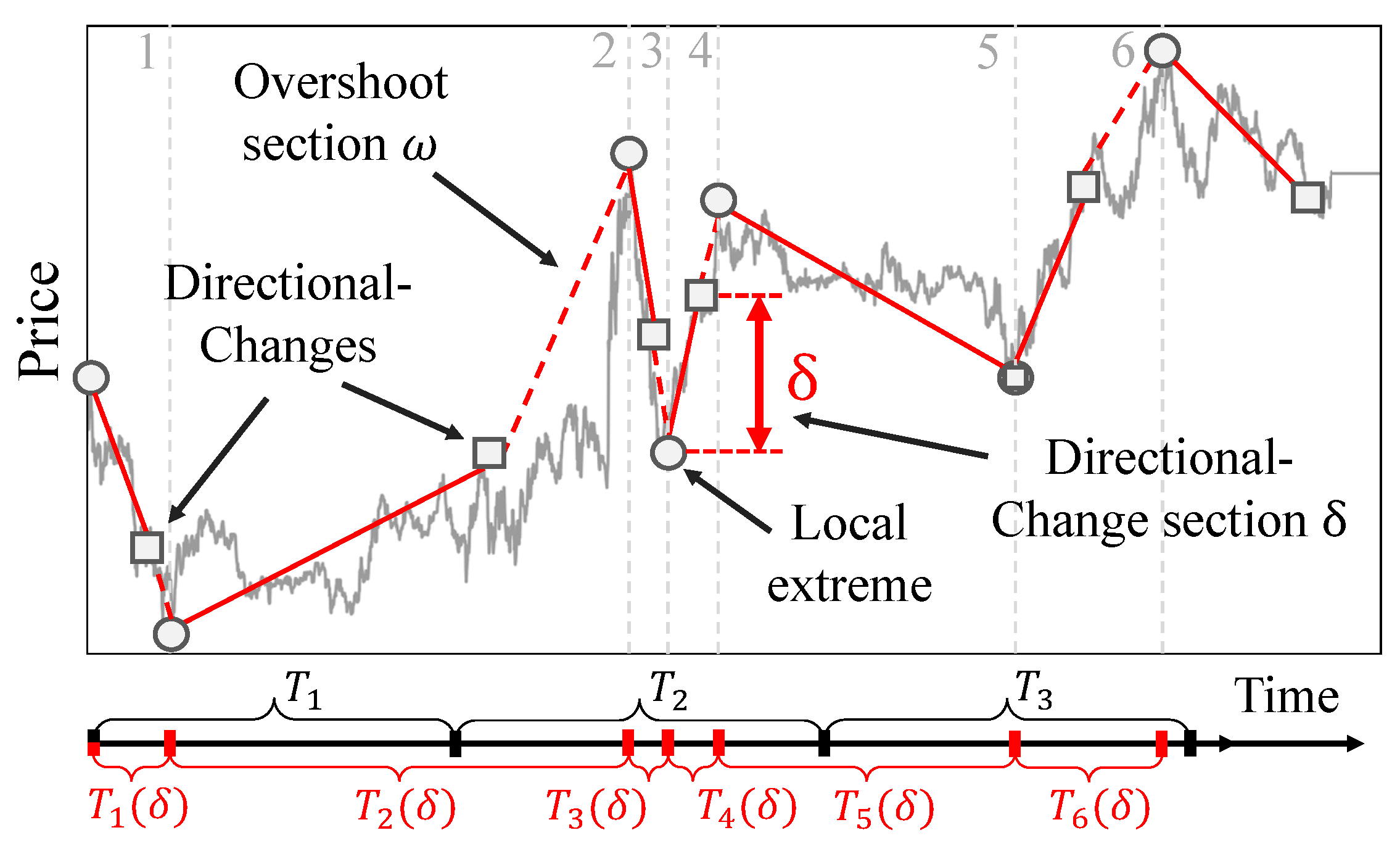
The concept of trend directional changes provided by Guillaume et al. (1997) is capable of connecting the continuous flow of physical time with the endogenous evolution of price returns. According to the event-based space proposed by Guillaume, only a sequence of price trends continuously alternating in direction has to be considered. The price curve gets dissected into a collection of alternating drawups and drawdowns or trend rises and trend falls correspondingly. Each elementary trend ends once a new price curve reversal is observed. Continuous price moves towards the direction of the latest trend change are called overshoots. The current state of the system changes only at the moments when the trend of the given size reverses its direction. Thus, the set of intrinsic events is decoupled from the flow of physical time. Instead, it depends only on the size of considered drawups and drawdowns labelled by the threshold . An example of a price curve dissected into a collection of directional changes is provided in Figure 1.
The density of directional-change intrinsic events depends only on the price curve evolution and the considered trend size. The stochastic nature of price evolution results in the phenomenon depicted in Figure 1: non-equal number of intrinsic events (empty squares) correspond to the equal periods of physical time. The physical interval contains only the end of the Section 1 (sections coincide with the intrinsic events and are separated by the dashed vertical lines) while the equal interval hosts three segments, namely . This property of directional-change intrinsic time can be engaged as the efficient noise filtering technique: the intrinsic time ignores price changes between directional change. At the same time, it allows us to efficiently capture the most relevant to risk management information: precise moments of all trend changes. The equally spaced time intervals typically employed in the financial analysis are not capable of doing anything of the above: price timestamps, evenly spaced through periods , and , do not contain information on the extreme price curve activity located in the period . This disability of the traditional price analysis techniques over stochasticity of the market’s activity develops into volatility estimators that are too stiff and biased.
The concept of directional-change intrinsic time, applied for studying historical price, returns reveals multiple statistical properties of high-frequency markets. Guillaume et al. (1997) were the first researchers to uncover a scaling law1 relating the expected number of directional-changes observed over the fixed period to the size of the threshold . Mathematically:
where and are the scaling law coefficients. Glattfelder et al. (2011) employed the directional-change framework to discover 12 independent scaling laws which hold across three orders of magnitude and are present in 13 currency exchange rates. Later Golub et al. (2017) described a successful trading strategy exploiting a collection of tools build upon directional-change intrinsic time. The proposed strategy is characterised by the annual Sharpe ratio greater than . The persistence of revealed scaling laws became the base elements for the tools designed to monitor market’s liquidity at multiple scales (Golub et al. 2014).
4. Seasonality
4.1. Traditional Markets
The returns seasonality is the well-known statistical characteristic of developed markets such as FX and stocks. Rozeff and Kinney (1976) studied the comprehensive set of historical stock data which spans from 1904 to 1974 and found a higher mean of return in the January distribution of returns compared with most other months. They also underline noticeably high mean returns in July, November, and December, and low mean returns in February and June. Gultekin and Gultekin (1983) empirically examined stock market seasonality in major industrialised countries. They aimed at investigating the existence and the shape of the stock market seasonality pattern in foreign securities markets. The confirmed seasonal patterns in the stock returns supplied the further understanding of the seasonality anomaly. Seif et al. (2017) studied seasonal anomalies in advanced emerging stock markets and provides re-examination of the markets efficiency. The authors did not find the confirmation of the January effect but confirmed the month of the years, the day of the week, the holiday, and the week of the year effects. The recent work Fang et al. (2018) presents a strong link between school holidays and market returns across 47 countries. The authors demonstrate that the returns in the month after major school holidays are 0.6% to 1% lower than at other times. The provided evidence states that post-school holiday small returns are explained by the investors’ inattention during these periods. The reduced attention results in news effects being incorporated noticeably slower into prices than within the active trading periods. We also underline the relevance of other research works on the stock market seasonality: De Bondt and Thaler (1987); Keim (1983); Zarowin (1990), among others.
Daily, weekly, and annually seasonality patterns are also inevitable components of the set of FX stylised facts. Müller et al. (1990) analysed four foreign exchange spot rates against the USD over three years. Authors’ intra-day and intra-week analysis show that there are systematic variations of volatility present even within business hours. They also discovered daily and weekly patterns for the average bid-ask spread. Dacorogna et al. (1993) studied daily and weekly FX seasonality patterns from the geographically distributed trading point of view. The trading activity divided in three general components (East Asia, Europe, and America) was approximated by a polynomial activity function during business hours. The combined model was closely fitted into the empirical volatility (activity) seasonality data. The authors found that strongly seasonal activity autocorrelation can be approximated by the hyperbolic function. Bollerslev and Domowitz (1993) examined behaviour of quote arrivals and bid-ask spreads for continuously recorded deutsche mark-dollar exchange rate data over time, across locations, and by market participant. The authors find the relation of the considered information to the seasonality patterns typically observed in the deutsche mark-dollar exchange rate. Ito and Hashimoto (2006) showed U-shaped intra-day activities of deals and price changes as well as return volatility for Tokyo and London participants of USD/JPY and EUR/USD markets. The authors also note that the U-shape was not found for New York participants. A set of well-known seasonality factors was confirmed: the high activities at the opening of the markets, high correlations between quote entries and deals, and higher trading activities associated with narrow spreads.
The seasonality of the rapidly evolving cryptocurrency domain is still insufficiently studied in the financial world. The next section unwraps some of the facts about cryptocurrencies and presents outcomes of the previous studies which have to be considered in the current work.
4.2. Bitcoin Seasonality
Bitcoin is the first successful pioneer in the crypto domain. It is also the most famous representative of the cryptocurrency markets. Bitcoin was described by Nakamoto (2008) and created in 2008 as an alternative to the classical financial system. The cryptocurrency was rapidly tagged as the “peer-to-peer version of electronic cash”. Bitcoin and its underlying technology, blockchain2, swiftly gained attention from the technologically savvy community and media. The peer-to-peer payment systems soon became one of the most debatable topics at all levels of modern society. Over a thousand alternative cryptocurrencies, based on the similar cryptography concept (Roy and Venkateswaran 2014), emerged since the time Bitcoin was invented. Some part of them became accessible for trading at various electronic venues also known as crypto-exchanges3.
In contrast to the traditional FX market, cryptocurrency trades happen 24 h per day and seven days per week, independently of the holidays and seasons. Additionally, cryptocurrency trading activity is more uniformly distributed across the globe. There are not many big geographically segregated financial institutions where trades happen according to the working schedule (in contrast to the global FX trading centres described in Dacorogna et al. (1993)). There is still the limited acceptance of this new financial instrument by international organisations with access to sizable funds4. As result, the seasonality patterns prevalent in the world of cryptocurrencies could be incomparable with the ones typical for the FX or stock markets. High volatility has been one of the most pronounced characteristics of the Bitcoin markets (see, for example, Dyhrberg (2016)). Bitcoin’s trend drastically changes and their persistence indicates the aggregated expectations and trading actions of all market participants. Unstable trends also reveals the Bitcoin price sensitivity to exogenous stress factors. The high scale of Bitcoin trend changes attracts researchers to employ modern technologies in order to foresee the future price dynamics (Shintate and Pichl 2019).
There are a few research works concerned with the statistical properties of cryptocurrency markets. Sapuric and Kokkinaki (2014) analysed realised volatility of Bitcoin returns within a 4-year time interval to understand what the prime characteristics of its price activity are. They confirmed Bitcoin’s high volatility, but emphasised that traded volume should be taken into account when computing the precise value5. The authors compared Bitcoin with conventional financial instruments, including gold, and several national currencies. They demonstrated that the calculated volatility significantly decreases when the traded volumes are included in the model.
Haferkorn and Diaz (2014) studied seasonality patterns of the number of payments performed in three cryptocurrencies: Bitcoin (classified as a worldwide payment system), Litecoin (open source software project), and Namecoin (decentralised name system). Their research confirmed that the monthly or yearly seasonality is not typical for the crypto market. The only robust weekly pattern was found in Bitcoin prices. Litecoin and Namecoin had weak or no patterns at all. The authors state that there is also no significant correlation between the returns of observed exchange rates. Authors speculate about the reason of this phenomenon. They say that these cryptocurrencies have similar core architecture, but they all have been created to serve specific needs.
de Vries and Aalborg (2017) made another attempt to discover Bitcoin seasonality patterns. They analysed daily traded volume, daily transaction volume, and Google trends (the number of searches for the word “bitcoin”). The author also inspected the seasonality of the number of transactions performed from individual blockchain accounts. All of the measurements demonstrated no particular periodicity.
Eross et al. (2017) gave a more positive answer on the existence of the most famous cryptocurrency intraday seasonality. The authors investigated Bitcoin returns, volume, realised volatility, and bid-ask spreads to reveal several intraday stylised facts. A significant negative correlation was found between returns and volatility. Volume and volatility were shown to have a considerably positive correlation. The authors attribute such patterns to the European and North American traders, as well as the insufficient number of market makers in the whole crypto space.
The seasonal heteroscedasticity affects the results of statistical studies of intraday and intra-week price properties. The rapidly evolving electronic high-frequency trading is highly affected by the exchange rate seasonality properties too (Cont 2011b). Therefore, the returns’ seasonality has to be treated at the first priority.
More information on order patterns in time series can be found in the work Bandt and Shiha (2007). The authors determine probabilities of order patterns in Gaussian and autoregressive moving-average processes, which can be directly applied to the financial time series analysis.
5. Data
Three FX exchange rates were used in the work: EUR/USD, EUR/JPY, and EUR/GBP. The covered time interval is from January 2011 to January 2016 and includes 109,069,357, 134,737,397, and 88,704,676 ticks correspondingly. The source of the data is the JForex trading platform developed by the Swiss bank and marketplace Ducascopy, which provides various types of market data in the highest resolution6.
Bitcoin price changes observed at the Kraken crypto-exchange were downloaded from the Bitcoincharts online platform supplying financial and technical data related to the Bitcoin network7. The studied time interval is from January 2014 to April 2018 and includes 4,778,429 ticks.
The stocks market is represented in this work by the index that currently comprises 505 common stocks listed by 500 large-cap companies on the US stock market: S&P 500 (with the ticker SPX500). The high-frequency data has been downloaded from the JForex platform too. The selected dataset spans from January 2012 to January 2017. The total number of ticks is 38,931,943.
There is a substantial difference in the number of ticks in time series used in the work. The difference reflects the distinct activity in the selected traditional and novel markets. That discrepancy does not undermine the further results since our goal is to apply the novel volatility measurement techniques, which is agnostic to the number of ticks per period of time (see Section 3). Moreover, the discrete price impact on the instantaneous volatility will be described in Section 7.3. The same is correct for the slight time-span shifts. The compatibility of the results is not affected: the designed experiments aim to depict the statistical properties of the volatility seasonality and not to compare price behaviour at any particular historical moment of time.
The fully functional code used in the project can be downloaded from the author’s GitHub repository8.
Inner Price
Any collection of historical prices typically assumes two values: the best bid (buy) and the best ask (sell). These prices are collected from the complete order books specific for the given exchange. The order books contain all clients orders submitted in the market at the given moment. The non-zero price difference between the best offers on the sell and buy sides, called spread, indicates the level of a market’s liquidity (Bessembinder 1994; Dyhrberg et al. 2018; Menkhoff et al. 2012). It also has a direct connection to realised volatility (Bollerslev and Melvin 1994), and is an indicator of the transaction cost (Hartmann 1999). Another role of the spread is to show the extent of uncertainty the market has on the fair price of the traded asset. The size of the spread constantly changes over time, together with the level of uncertainty. This fact does not allow us to employ only bid or ask prices to study properties of the whole market at the micro level since some part of the information is in the risk to be lost while analysing intraday data. The average of these two values (mid-price) is also not the best alternative since it does not keep the knowledge on the size of the current spread. Therefore, an alternative measure should be chosen to apply the directional-change algorithm to the real data analysis.
The trend-dependent concept of inner price was selected to resolve the spread issue. Inner price, specific for the given moment of time, is defined as the bid or the ask price depending on the direction of the current trend. In other words, it is the price where the spread is deduced. The following example demonstrates details of the concept. According to the directional-change algorithm, one should wait for the price increase by percents from the local price minimum to register a new directional change if the current trend is downward. In this case, the value of the inner price coincides with the best price on the offer side of the order book, that is, the ask price. A new intrinsic event will tick only when the distance between the latest bid price and the inner price reaches the size of the chosen directional-change threshold . Alternatively, the inner price takes the value of the best bid price, and the distance is measured between the newest ask and the extreme if the current mode is upward.
6. Methods
Theoretical researchers mostly rely on the Brownian motion as the proxy for price returns of real financial markets (one of the most famous examples is the work of Black and Scholes (1973)). The analogy between historical price moves and changing coordinates of an ensemble of molecules in thermodynamics is the motive behind this common approach. Osborne (1959) shows in the classical work that the steady-state distribution of log-returns in the stock market is the probability distribution for a particle in Brownian motion. It is important to emphasise that at the telegraph-driven time of Osborne’s publication (1959) the structure and the dynamic of the market was very different from the ones typical for our modern digital world. The present-day trading has almost completely moved to the digital online space instead of the physical trading floors where all deals happened more than a half a century ago (see Harris (2003) for the historical endeavour on the evolution of trading and exchanges). In this space, a signal can easily propagate through international borders with the speed of light. It stipulated the majority of trades to happen in a fully automated way. The significantly bigger diversity of the market participants and the ability of the high-frequency trading made the financial stylised facts more important today than ever. The stylised facts describe the deviations of real price returns from the theoretical Brownian motion (see Cont (2001a) for the set of stylised empirical facts). Nevertheless, in our work, we will operate with Brownian motion as the core for the analytical part of the research.
The choice of Brownian motion, employed in this work, is justified by two reasons. First, the statistical properties of the number of directional-change intrinsic events, studied in this work, is agnostic to the flow of physical time. Second, the divergence of empirical results from the properties of the selected model, if any, helps in understanding the features of the real markets better.
6.1. Waiting Time
We model the set of prices as an arithmetic Brownian motion with trend and volatility :
In terms of the directional-change intrinsic time framework, denotes the time for an upward directional change of the size to unfold. In other words, it is the time interval which passes until the price increases by percents from the local minimum . Technically:
where
Similarly, is the time of a downward directional change of the size :
where
Both of these equations are also known in the literature as waiting times of drawups and drawdowns (see Section 1). It is shown in Landriault et al. (2015) that expected times of a drawup and a drawdown depend on the volatility and the trend of the drifted Brownian motion. It can be mathematically expressed as
and
Using the Taylor expansion and letting , one can recover that in the case with no trend the equation simplifies to
These equations establish a scaling law dependence between waiting times of a directional change, volatility, and the selected size of the directional-change threshold. Indeed, in the analysis of Glattfelder et al. (2011) it was empirically found that in the FX market the average waiting time is proportional to the second power of the directional-change threshold used to identify alternating trends:
6.2. Number of Directional Changes
Let denote the number of drawdowns of the size observed within the time interval in Brownian motion process with parameters and . Since the sequence , ,… is the sequence of non-negative, independent, and identically distributed random variables, the sequence where is the renewal point process. Thus, can be considered as the renewal counting process and its values can be found applying the Theorem 6.1.1 of Rolski et al. (2009) (Landriault et al. 2015) to the waiting time Equation (11):
Correspondingly, the expected number of drawups takes the form
Equations (14) and (15), combined together, give the estimate of the number of directional changes consequently following each other:
The expression is simplified in the trend-less case () to the following form:
The theoretical dependence of the number of directional changes and the properties of underlying process resemble the empirical observations of Guillaume et al. (1997). The authors mention there that (for ).
Monte Carlo statistical tests were performed to numerically verify the accuracy of Equations (10), (11) and (16). Results of the tests are provided in Table 1. We selected only positive trend values since the equations are symmetrical with respect to the direction of the trend. Values in Table 1 exhibit high similarity of both empirical and theoretical results.
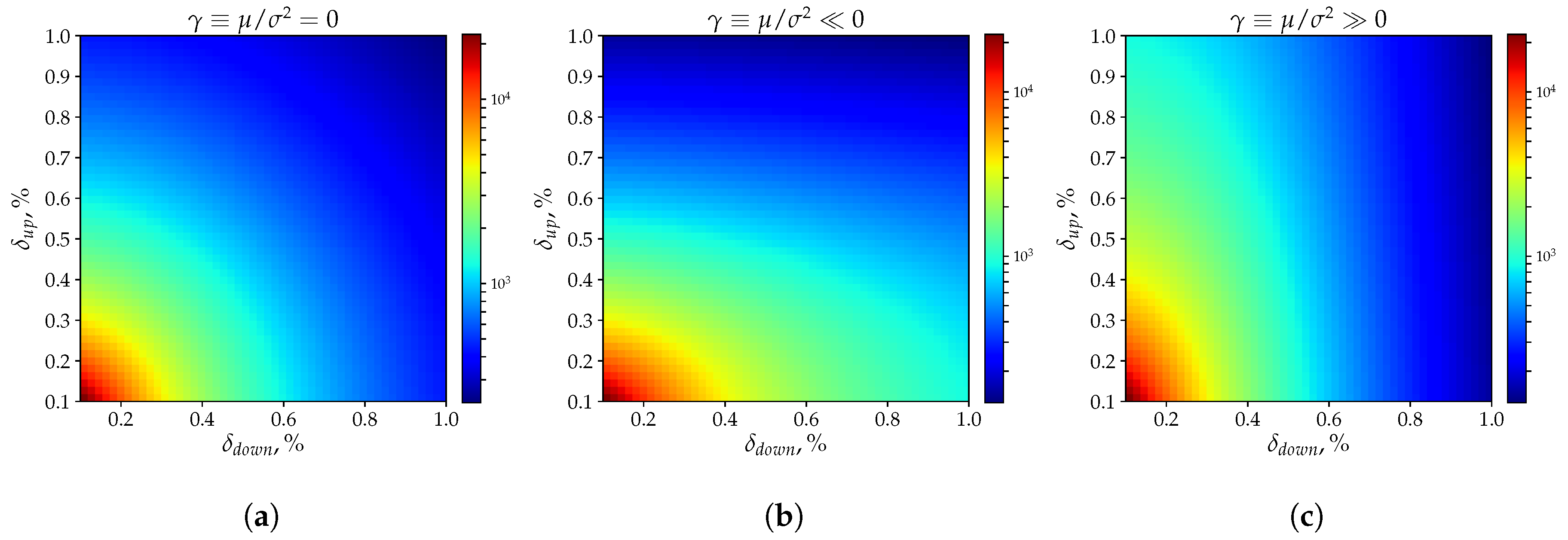
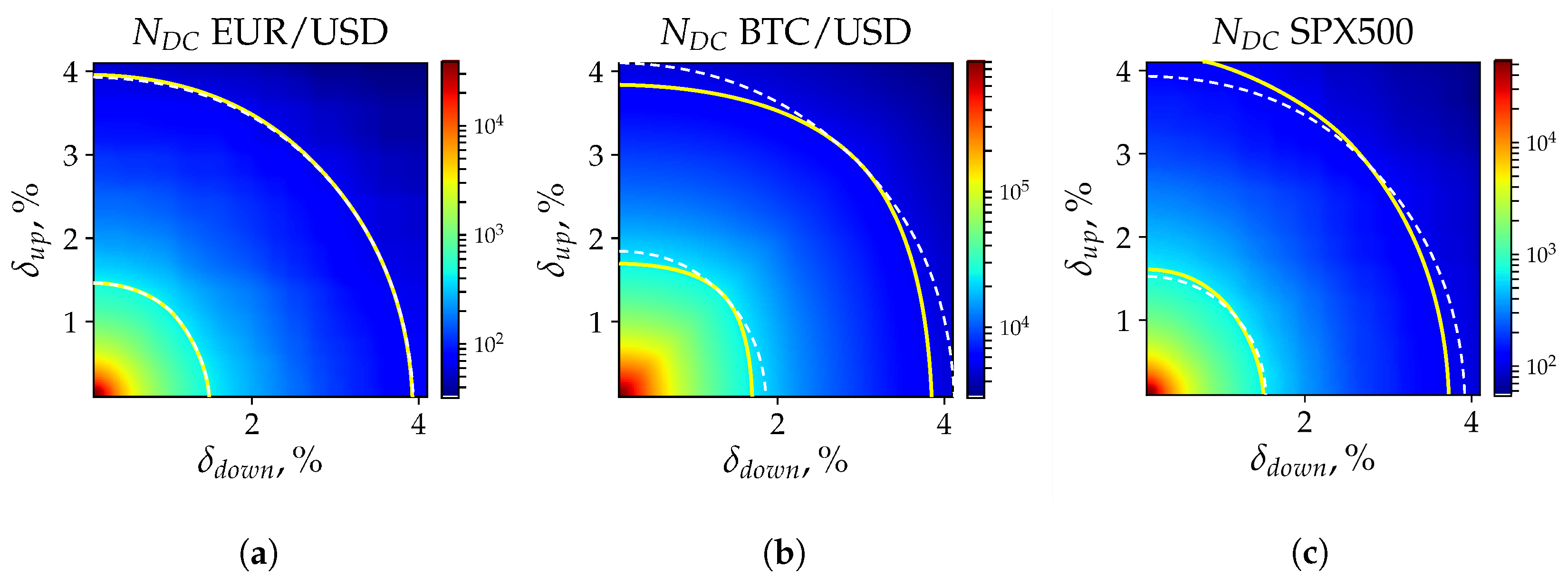
The meaning behind the provided equations is that the absolute size and the ratio of directional-change thresholds used to dissect a price curve into a sequence of upward and downward trends affect the frequency and the total number of events registered within a given time interval. It follows from Equations (14) and (15) that the combination is the crucial factor affecting the expected number of intrinsic events9. We check the number of directional changes registered by a couple of thresholds in three extreme scenarios: (Figure 2a), (Figure 2b), and (Figure 2c). A diverse set of dissection procedures was applied to the randomly generated time series defined by the parameters . All results were composed as a heatmap where each point corresponds to the number of directional changes observed by a pair of thresholds (Y- and X-axis of the plots) in a time series of the given length (Figure 2).
Panel 2a in Figure 2 corresponds to the set of experiments where the Brownian Motion trend is equal to zero. It follows from Equation (17) that in such conditions the value should be constant along circular contours for . The colour gradient in the provided picture confirms the noted dependence. It is shown in panels 2b and 2c of Figure 2 that the circular contours transform into ellipses when the “adjustment coefficient” is significantly smaller or significantly bigger than zero. This phenomenon can be interpreted in the following way: if is the expected number of directional changes registered in the drift-less time series of given length and characterised by the fixed then for any greater or smaller than zero there is always such a couple of non equal thresholds that
In other words, any process characterised by a certain degree of persistent trend could be treated as the one without the trend by tuning the size and the ratio of selected directional-change thresholds. The property is essential for risk management techniques constructed on top of directional-change intrinsic time approach. An example of real application of this fact is provided in Golub et al. (2017). The authors employed asymmetric thresholds to design an optimal inventory control function sensitive to the significant price trend changes.
6.3. Instantaneous Volatility
The volatility size of the financial time series is an inevitable component of any financial risk analysis. Therefore, a clear understanding of the way how volatility changes over time is particularly important for risk management and inventory control problems. Classical volatility estimation methods, also called “natural” or “traditional” estimators (Cho and Frees 1988)10, primarily rely on physical time as the persistent measure of the intervals when the price returns should be computed. The fact that the variance of returns on assets tends to change over time creates obstacles on the way of employing the “traditional” volatility estimators. The changing variance, also known as the stochastic volatility, became a cornerstone for multiple research works (for example, Aı and Kimmel (2007); Andersen and Lund (1997); Barndorff-Nielsen and Shephard (2002); Campbell et al. (2018) and many others).
Values, computed by “natural” estimators, dominantly correspond to the integrated volatility of the studied process. The integrated volatility describes the averaged price activity over non-zero time intervals. Alternative estimators, designed to reveal the size of the volatility as the time interval approaches zero (instantaneous volatility), are mostly based on Fourier analysis11 and require extensive computation efforts (see Chapter 3 in Mancino et al. (2017)). Therefore, new methods, capable of describing the price evolution independently of the flow of the price in physical time, should be employed to overcome the existing volatility estimation difficulties.
The directional-change intrinsic time concept is by design agnostic to the speed of the price change. Risk-management tools, based on top of the concept, automatically adapt their performance to treat the changing price activity better. This property of directional-change intrinsic time, together with analytical Equations (16) and (17), bring the idea of a new volatility estimator devoid of the shortcomings of the equidistant time in finance. It follows from Equation (17) that the volatility can be estimated for a trendless time series by counting the number of directional changes within the time interval :
We use the superscript to distinguish the volatility computed through the directional-change intrinsic time from volatility computed by the traditional estimators. The latter we will mark by .
Equation (19) solely computes the volatility part of the Brownian proces. That contrasts the “natural” volatility estimation techniques where the entire stochastic part is typically measured. That stochastic factor includes the noise component . Therefore, the directional change approach employed for volatility measurements can be classified as the true estimator of the instantaneous volatility. Further, we apply Equation (19) to study changing dynamic of financial time series throughout one week. We reveal volatility seasonality patterns of three FX exchange rates, crypto market BTC/USD, and the stock index S&P500.
7. Results
Empirical properties of three distinct markets will be discussed in this section. We omit the EUR/JPY, and EUR/GBP exchange rates in some of our experiments due to the fact that their properties are greatly similar to the properties of the most traded FX rate EUR/USD. In this case, EUR/USD is selected as the representative exchange rate of the entire FX domain.
7.1. Number of Directional Changes
Equations (16) and (17) connect the expected number of directional changes with parameters of the underlying Brownian motion process. The evolution of real historical returns have properties similar to the Brownian motion. The evolution sometimes compared to the sequence of the free particle moves (see Section 6). Thus, similar counters shown in Figure 2 should be found in heatmaps depicting the number of directional changes empirically registered in real data conditional that the assumption of the normal distribution of real returns is true. EUR/USD, BTC/USD, and SPX500 exchange rates were taken to verify the statement by replicating the same experiment done with the Brownian motion before (Figure 3). A collection of 40 directional-change thresholds ranging from to defines the scale of the heatmap grid. Colour schemes, used for the plots, have different scales due to the significantly bigger number of directional changes per a period of time in the BTC/USD case. Yellow solid lines indicate the examples of the areas where the number of direction changes is constant. The selected for the examples deltas are (EUR/USD, Figure 3a), (BTC/USD, Figure 3b), and (SPX500, Figure 3c).
Curves in Figure 3a have an almost circular shape and are only slightly shifted towards the bigger values. This shift is present due to the downward trend experienced by the exchange rate from 2011 to 2016 (from $1.4 to $1.1 per EUR). BTC/USD exchange rate was much more unstable considering that the EUR/USD time series exhibited relative stability with no noticeable regime switches apart from the slow constant price depreciation. The price of Bitcoin grew with accelerating pace by more than 20 times in the second half of 2017 and then lost nearly of its value at the beginning of 201812. These significant trend changes are pronounced in Figure 3b by yellow contours notably deviated from the circular shape. The price roller-coaster caused considerable disparity of the number of registered directional changes and the ones predicted by Equation (17) (relevant to the trend-less case). As result, the solid price curves can be decomposed into two parts of independent ellipses similar to the ones observed for Brownian motion with non-zero “adjustment coefficient” (Figure 2b,c).
7.2. Realised versus Instantaneous Volatility
In the second experiment, we compared the annualised volatility computed by the traditional method (Equation (20)) and the volatility based on the observed number of directional changes (Equation (19)).
Returns are defined as logarithms of the price change between and measured over equal periods of time. The number of returns n depends on the selected time interval and equal to where T is the length of the entire tick-by-tick sample. Thus, the length of a sample can be computed ex-ante.
The whole set of returns was used to find the standard deviation of the time series. The measure is also known as realised volatility :
The directional-change method does not define the number of observations ex-ante in contrast to the traditional approach. According to Equation (19), the size of the directional-change threshold determines only the expected number of measures (or timestamps) in the data sample of the given length. It is also worth saying that the price moves of the highest frequency, tick-by-tick, do not appear over any predefined period. They occur together with the flow of new orders in the market. The flow, initiated by thousands of independent traders’ demands, not synchronised with any periodical process. Thus, the time distance between two consecutive ticks can be represented by a fraction of a second as well as by several minutes. The equally spaced timestamps used to calculate returns for the “natural” estimators have a high chance to happen not at the moment of a new price change. The additional decision should be made on whether the historical price located before the timestamp or right after it should be selected to compute the corresponding return. The directional-change intrinsic time, in turn, directly reacts to the changes of the price levels. This flexibility of the intrinsic time makes it possible to use the data of the highest frequency: tick-by-tick prices.
Specifications of tools used to estimate volatility can affect the experiments results (Müller et al. 1997). Four increasing time intervals , where , were selected to define the distance between each pair of consecutive prices and used for the “natural estimator”: min, min, h, and day. The set of thresholds employed to investigate the directional-change approach can also be arbitrarily chosen. However, we selected them with the intent to compare the results of both experiments. For this reason, we used the number of returns in the data sample corresponding to each time interval as the target for the number of directional changes registered in the same data set. That is, the collection of four thresholds was selected in such a way that in the given time series the number of directional changes is approximately equal to the number of time intervals of the length . We utilised one of the scaling properties described in Glattfelder et al. (2011) to find the precise thresholds size. The scaling property has the name “time of total-move” scaling law (law 10 in the article). The total-move is composed as the sum of the directional-change (DC) and overshoot (OS) parts. The law connects the size of the threshold with the waiting time between two consecutive intrinsic events:
where and are the scaling coefficients. Equation (21) can be used to express the threshold in terms of the waiting time :
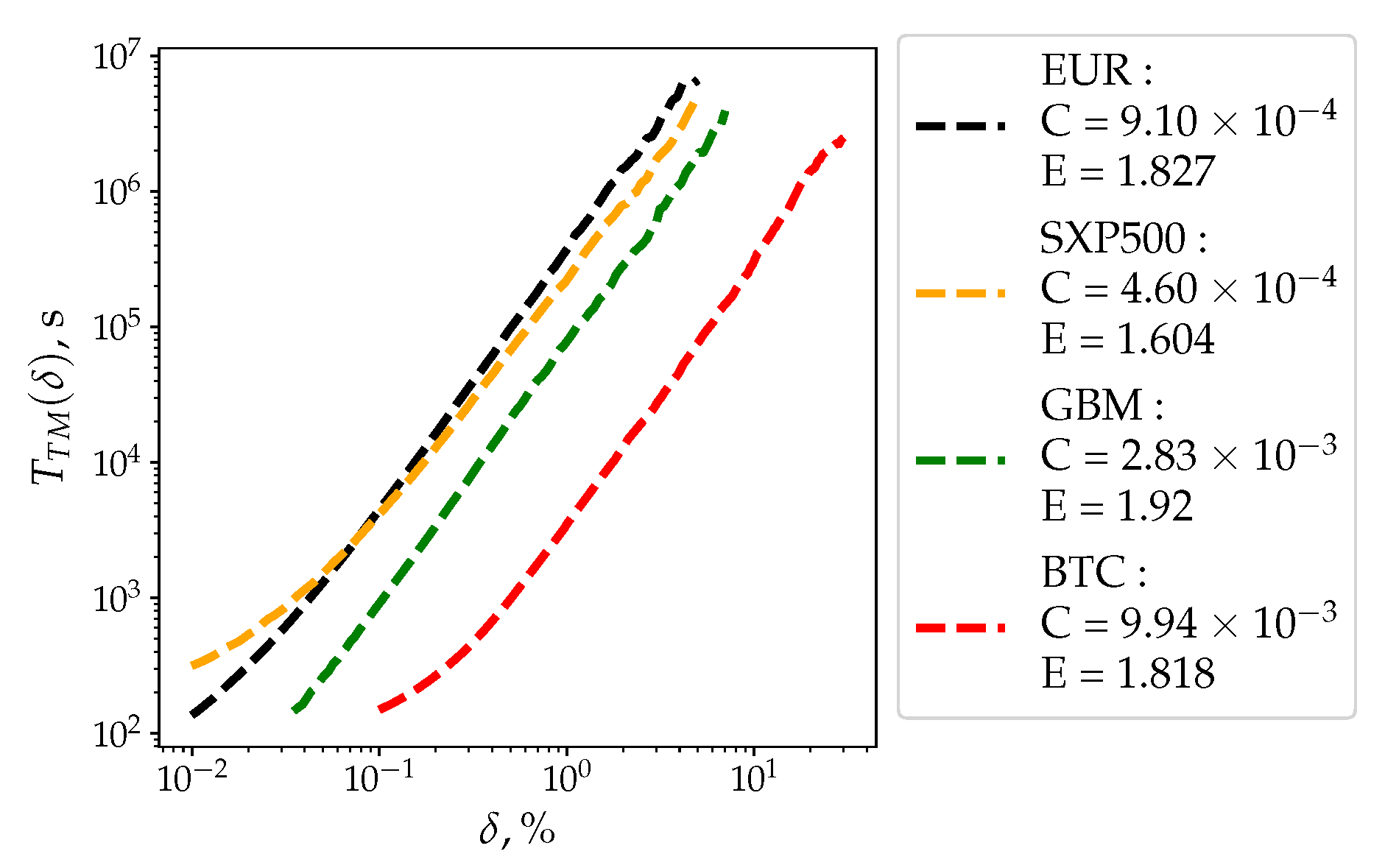
The currency average scaling parameters and computed in Glattfelder et al. (2011) are and 1.65 × 10⁻³, correspondingly. Putting these coefficients into Equation (21), one can calculate that thresholds reciprocal to the selected time intervals are: , , , and . It is worth mentioning that applied scaling parameters are relevant only to the FX market which was the object of the research in Glattfelder et al. (2011). To the extent of our knowledge, parameters specific to Bitcoin prices, as well as to the S&P500 index, were not mentioned in the scientific literature before. Therefore, as the first step, we obtained the parameters by studying the “time of total-move” scaling law of historical Bitcoin, and SPX500 returns. The log-log plot of waiting times versus the directional-change threshold size is provided in Figure 4. The red line marks BTC/USD scaling law and is shown together with black, yellow, and green lines computed for EUR/USD, SPX500, and Geometrical Brownian Motion (GBM) correspondingly. Settings of the latter are chosen to mimic returns typical for the FX market.
Total-move scaling law parameters, obtained in the experiment, exhibit distinct resemblance of the stylised properties of the traditional FX and SPX500, as well as the emerging Bitcoin markets. Scaling factors of EUR/USD, BTC/USD, and SPX500 are , , and , correspondingly. The coefficient specific for the BTC/USD pair is approximately 0.5% smaller than the one of EUR/USD. The coefficient of the SPX500 index is, in turn, is substantially smaller: by 9.9%. The same scaling factor of the GBM is the biggest among others: ( difference with EUR/USD). The parameter is noticeably distant from the parameters of the analysed exchange rates. We account the divergence to the non-normal distribution of real returns at ultra-short timescales (fat tails). The fat tails effect is pronounced in Figure 4 as the upward bend of the curves towards the beginning of the X-axis. The bends are read as the longer time needed for a total-move to unwrap than it is predicted by the linear part of the plot in the range of higher thresholds values. Linear regressions, built in the range of straight parts of the curves, are characterised by the scaling coefficients , which are close to the ones observed in GBM. The observed evidence is an additional confirmation of the “Aggregational Gaussianity” stylised fact13 typical for high-frequency markets (Cont 2001a). Scaling parameters of EUR/USD, BTC/USD, and SPX500 are 9.07 × 10⁻⁴, 9.94 × 10⁻³, and 4.60 × 10⁻⁴, correspondingly. These values are significantly different due to the unlike scale of the corresponding volatility. This volatility dependent scaling parameter is not critical for the current analysis and will be discussed in the future research works.
The goal of the experiment is to compare the volatility computed using the ”traditional” approach to the volatility based on the directional-change intrinsic time concept. Scaling law parameters and of historical BTC/USD returns were used to find the size of the directional-change thresholds, which would result in the average number of registered intrinsic events in the entire data-sample equal to the number of evenly spaced periods . Expressing the parameter from the Equation (21) we find that for BTC/USD the thresholds are: , , , . The values are about ten times bigger than the ones related to the FX market (mentioned above) because of the proportionally larger realised volatility.
The same procedure, described in the previous paragraph, was performed in order to find the corresponding thresholds for the SPX500 time series. The obtained values: , , , .
The set of selected time intervals and the complementary thresholds specific for each considered market were used to calculate realised and instantaneous volatility by traditional and the novel approach. We present in Table 2: average value of the realised volatility computed as the sum of all four measurements () divided by the number of experiments; its standard deviation ; average value of the instantaneous volatility computed by the novel approach ; the corresponding standard deviation ; ratios of both measures and . The last column of the table demonstrates the difference in the stability of results obtained by two measures.
The size difference of the realised and the instantaneous volatility is significant and is pronounced across all tested exchange rates (column ). The realised volatility computed in the “natural” way persistently exceeds the instantaneous volatility discovered via the novel approach. Only the two types of Bitcoin’s volatility appear to be different whenever the divergence grows up to in the case of SPX500. The striking difference is partially explained by the various discreteness of the employed data (which will be elaborated in the next section), and partially by the phenomenological properties of the selected markets (more on it in Section 7.4). This phenomenon is captivating especially taking into account that Bitcoin is particularly famous due to its oversized price activity. Its activity is clearly pronounced as the large standard deviation of the instantaneous volatility of BTC/USD pair (column ). Three FX exchange rates, having noticeably smaller realised volatility, are characterised by the wider range of the standard deviation values (column ). The ratio reaches the level computed for EUR/USD. In other words, the standard deviation of the EUR/USD instantaneous volatility is 50 times bigger than the realised volatility value.
7.3. Discrete Price Effect
The instantaneous volatility standard deviation computed for four different directional-change thresholds has an extremely high value (column in Table 2). This indicates that in contrast to the realised volatility capable of the scaling, together with the time interval , the instantaneous one does not scale together with the threshold size .
The price discontinuity typical for all real markets is the cause of the high standard deviation of the instantaneous volatility computed by the directional-change approach. Conventional exchange architecture restricts the price quotations to be a multiple of some constant, for example, of a USD. This discreteness caused substantial debates in the scientific literature with regards to the accuracy of the ”natural” estimators and on the extent to which they overestimate the actual volatility of the studied process (French and Roll 1986; Gottlieb and Kalay 1985). Equation (19) connects the number of directional changes observed per period of time and the instantaneous volatility and is built on the assumption of the continuous Brownian process. It has no adjustment factors to the discreteness of the analysed data. In reality, the directional-change intrinsic time does not precisely tick at the level where the size of the return is equal to the size of the threshold . Instead, in most cases, a new directional-change event becomes registered when the price has already jumped over the expected level. This discreteness effect becomes more pronounced when the size of the elementary price move (tick) is relatively big. That is, two factors contribute to the size of the instantaneous volatility of the discrete data-sample computed by the novel approach: the scale of the selected threshold and the tick size in the given sample (discreteness). Further, we provide results of a set of experiments where the impact of the price discreteness and the threshold size on the computed instantaneous volatility is observed.
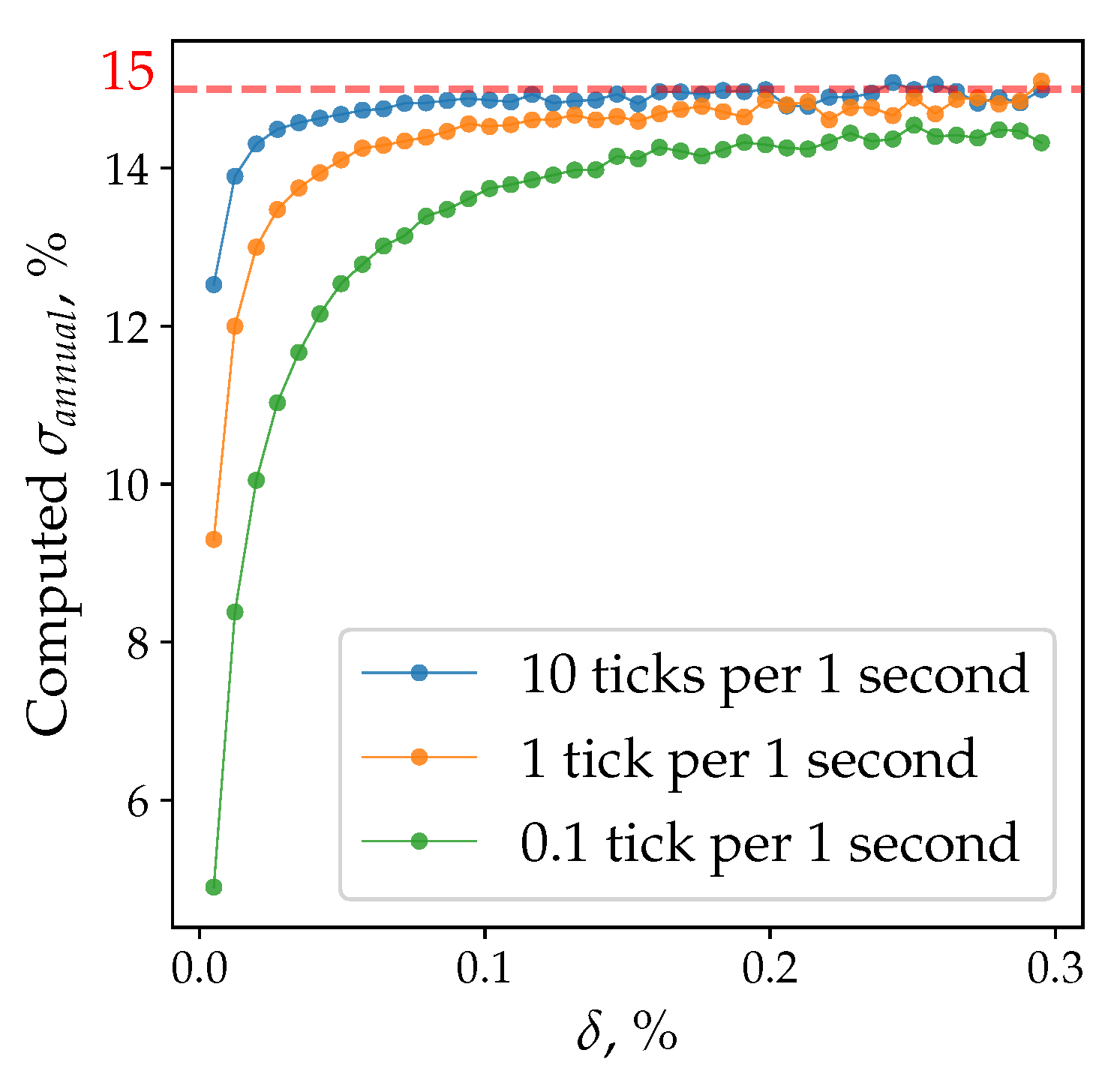
Three time series were generated by GBM with the various density of ticks per period of time. Variation of the number of price changes in the simulation is equivalent to changing the simulated tick size having fixed a one-year time interval and volatility of the generated process fixed to be . Forty gradually increasing directional-change thresholds were applied to all three GBMs. The thresholds range from to . We provide the plot of the computed instantaneous volatility of simulated time series in Figure 5. Two particular properties can be noticed. First, one brings the generated time series closer to the continuous process by making the size of a tick smaller (increasing the number of price changes per period in the sample). In this case, the values of the estimated instantaneous volatility become closer to the volatility embedded in the model. Second, bigger thresholds are less sensitive to the discreetness of the given set of prices. The slippage effect of the price jump over the expected intrinsic time level becomes less pronounced, and the obtained result also approaches the value when the tick size represents a small fraction of the directional-change thresholds. A more comprehensive analysis should be performed in further research works to bridge the gap between the realised and instantaneous volatilities.
7.4. Volatility Seasonality
Dacorogna et al. (1993) presented a weekly seasonality pattern of price activity in the FX market. The authors’ analysis is based on the assumption that worldwide trading happens at strictly separated time zones with several dominated cores and operates within specific trading hours. Such a physical distribution of traders is embodied in geographical components of the market activity and eventually becomes pronounced as the weekly volatility seasonality. We do not build a similar assumption in our work. Instead, the collection of observed historical returns is treated as the only source of information available for the analysis. Further, we discover and describe the seasonality pattern of instantaneous volatility typical for FX exchange rates, Bitcoin prices, and S&P500 index.
We divide a whole week into a set of 10-min time intervals (bins). There are 1008 equally spaced points located at the fixed distance from the beginning of each week. This is a significantly larger number than the one used in the work Dacorogna et al. (1993) (168 points spaced by one hour intervals). We can afford this decreased granularity thanks to the more detailed historical time series employed for the experiment: instead of 12 million ticks for 26 exchange rates, we have on average 100 million ticks for each of the FX pairs. For each bin, the average number of directional changes will be computed.
The following series of steps allowed to construct the seasonality pattern. First, we run all historical tick-by-tick prices through the directional-change algorithm with the specified threshold . As soon as a new intrinsic event becomes registered, we check within which out of 1008 bins it happened. We add to the number of directional changes corresponding to that time interval. When there are no prices left in the historical time series, we find the average number of intrinsic events per each bin. Equation (19) is then applied to compute the corresponding instantaneous volatility. Considering the five-year-long historical data, the obtained average is based on nearly 250 observations. Calculated instantaneous volatility values should be later normalised by the number of years and the length of a bin to get the annualised volatility specific for each bin of the week.
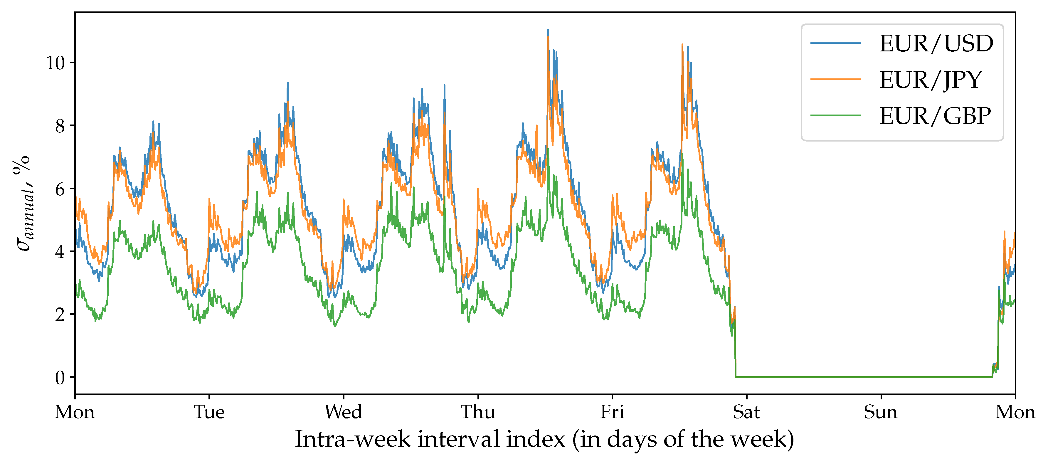
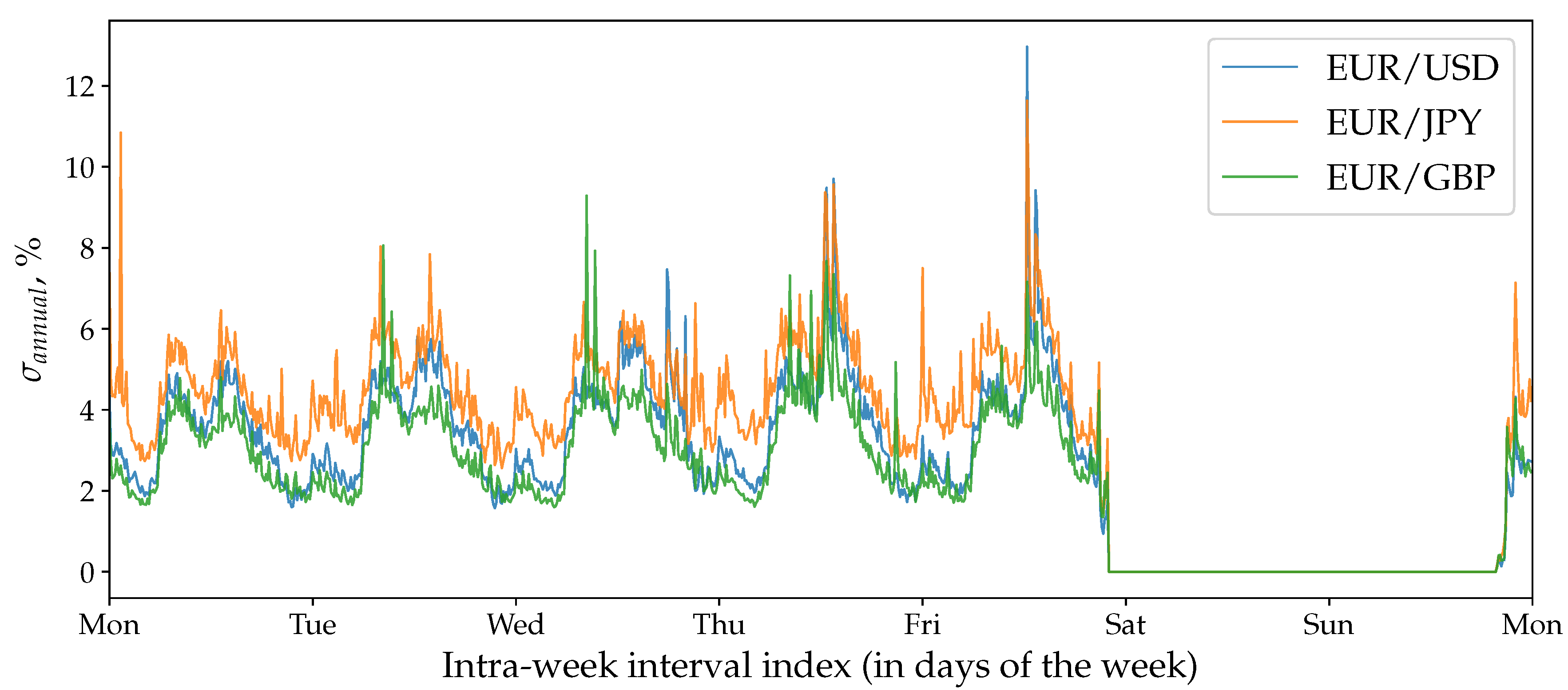
We select the threshold for the first experiment with FX exchange rates. The average number of directional changes in a week registered by a threshold of this size is approximately equal to the number of 10-min long bins in it (1008). The reconstructed instantaneous volatility seasonality pattern of the FX pairs is shown in Figure 6. The pattern is notably stable across all tested exchange rates and is similar to the one demonstrated in Dacorogna et al. (1993).
We provide results of the same experiment where the “traditional” volatility estimator (Equation (20)) was employed to reveal the seasonality patterns of the FX exchange rates in Figure 7 and of BTC/USD in Figure 8. In contrast to the volatility seasonality pattern computed using the directional-change approach (Figure 6), the “traditional” pattern is less affected by the frequency of ticks per period of time specific for each studied time series. The difference between the average realised volatility across a week of the most active pair (EUR/JPY) and the least active (EUR/GBP)14 is equal to . The same difference of the instantaneous seasonality (Figure 6) is bigger and equal to . The “traditional” estimator of the realised volatility seasonality demonstrates more rapid changes in the consecutive bins values. Local maximums at the beginning and the end of a day are considerably abrupt. The reason for this is that the directional-change intrinsic time captures the part of the volatility of the underlying process free of the noise component by ignoring the overshoot part of each trend move. The exact form and scale of the noise component and its connection to the overshoot section of the directional-change intrinsic time is a topic for future research work.
Assets traded in the crypto market have several specific properties which make them noticeably different compared to the traditional financial instruments such as FX exchange rates. Among the characteristics are: open trading within weekends and holidays; the absence of isolated physical trading centres where working hours are fixed; still low acceptance of the emerging market among professional traders. The outlined differences are endorsed by the history of technologies employed in the traditional FX and the emerging crypto worlds. The first one has originated in times when the trading happened in person and the settlement assumed the actual physical assets delivery. The trading organically evolved over time and became digital thanks to the internet expansion. Nevertheless, old properties, such as the governmental and the middle-man controls, have never been removed from the list of the accompanying FX markets design features. Bitcoin, in turn, has been designed as the alternative of the traditional financial system. It benefits from the blockchain technology by endorsing the principles of equality, openness, and accountability. We studied the historical prices of Bitcoin to investigate whether these specialities have any considerable impact on the BTC/USD instantaneous volatility seasonality pattern.
We apply the same threshold size used in the FX experiment to compare the seasonality patterns of Bitcoin and EUR. The obtained seasonality pattern put on top of the EUR/USD seasonality is presented in Figure 9. As can be seen from Figure 9, the periodical shape of Bitcoin’s curve is much less pronounced in contrast to EUR/USD. Its standard deviation computed within a week is . It is roughly four times smaller than the standard deviation of the EUR/USD pattern (equal to ). Surprisingly, the intra-day maximums and minimums of Bitcoin seasonality do not precisely coincide with those observed in the traditional market. They are shifted towards the time intervals where European and American markets contribute the most to the geographical pattern (as disclosed in Dacorogna et al. (1993)). This observation confirms the one provided in Eross et al. (2017). That is particularly interesting since Asian markets are known for their substantial contribution to the cryptocurrency trading volumes. The fact that China has ruled that financial institutions cannot handle any Bitcoin transactions could be the reason of the observed phenomenon (Ponsford 2015). Instantaneous volatility over weekends is slightly lower than within the middle part of the week and is practically equal to Monday’s activity. We attribute the observed facts to the mentioned above non-traditional characteristic of the cryptocurrency market.
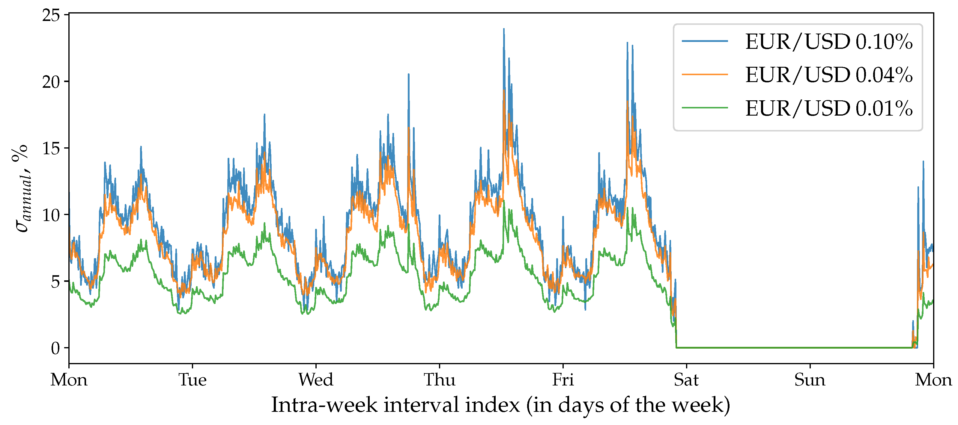
As it was shown before, the instantaneous volatility computed by the novel approach directly depends on the size of the selected directional-change threshold (Figure 5). To examine the threshold size impact on the seasonality pattern of the real data, we arbitrarily selected the following set of values: . The same algorithm described above was applied to reconstruct the volatility seasonality pattern for the FX pair EUR/USD (Figure 10) and SPX500 (Figure 11). The seasonality patterns shift toward higher volatility values when the size of the threshold is bigger. The observation is in line with the results of the experiments on GBM (Figure 5). Average values of EUR/USD seasonality curves computed with thresholds equal to and are correspondingly and times higher than the values computed with . The dependence of the seasonality smoothness on the size of the directional-change threshold become vividly pronounced: the seasonality curve constructed with the smallest threshold in the set is much sleeker (less wander) than the rest of the curves. This phenomenon should urge researchers and practitioners to select directional-change thresholds according to their needs very carefully while employing the directional-change technique.
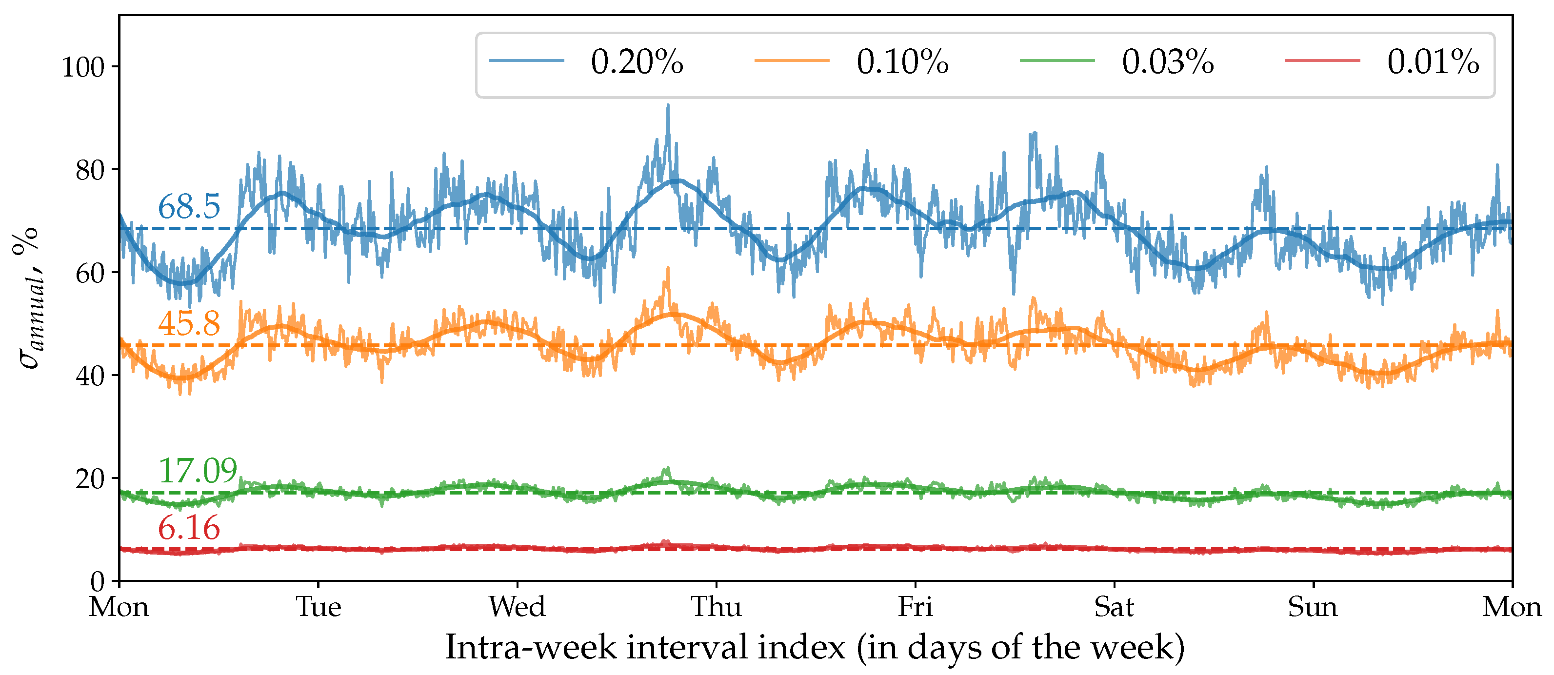
According to Table 2, realised volatility of Bitcoin returns computed in the “traditional” way is about nine and six times bigger than the analogous volatility of the FX and SPX500 exchange rates (column ). Besides, the retrieved sample of historical BTC/USD prices has million ticks per year, which is times smaller than the number of ticks per year in the EUR/USD case (about 20 million). As a result, the choice of the directional-change threshold has a much more significant effect on the average BTC/USD instantaneous volatility. We demonstrate results of four experiments where different threshold sizes were employed to reveal the seasonality patterns in Figure 12. The same was used as the reference for the set of all arbitrary selected thresholds: . As it can be seen from Figure 12, the increase in the size of causes the corresponding increase in the volatility level around which the seasonality patterns oscillate. The levels of the seasonality distribution for are , , and times bigger than the value corresponding to the smallest threshold . The biggest lifts the value up to the level of (which is still smaller than the realised volatility presented in Table 2 ()).
7.5. Volatility Autocorrelation and Theta Time
The shape of the persistent instantaneous volatility seasonality patterns computed for the FX and SPX500 exchange rates changes with clear daily periodicity. This observation suggests that there should be a strong autocorrelation of the instantaneous volatility over time. The connection of the number of directional changes and the volatility value (Equation (19)) translates into the autocorrelation of the number of directional changes. We examined the autocorrelation function (ACF) of the number of directional changes observed within each bin of a week to check the assumption. The results of the experiment made for the FX exchange rates are provided in Figure 13. The same size of the directional-change threshold used to reveal the seasonality distribution was employed. A remarkably stable pattern was found where daily and weekly seasonality is easily recognisable. The ACF function of FX exchange rates discovered in our work is highly similar to the results provided by Dacorogna et al. (1993). Nevertheless, there are clear differences between the FX autocorrelation patterns in our work and in the work of Dacorogna et al. (1993). The ACF of the number of directional changes computed through time lags defined in physical time does not cross the zero level for a much more extended period. It is consistently positive with lags even greater than several weeks. The curve representing the ACF of EUR/JPY has the smallest amplitude (smallest variability). In contrast, curves of EUR/USD together with EUR/GBP invariably follow the same pattern shifted up in the case of EUR/USD.
The SPX500 time series ACF has a similar shape to the shape of the FX market ACF. Two distinct properties can be noticed: the higher ACF amplitude and the faster decay. The exact level of decline of all exchange rates will be discussed a few paragraphs later.
The BTC/USD exchange rate seasonality pattern, characterised by much less pronounced instantaneous volatility, has also been tested in order to get the shape of the autocorrelation function. The results are presented in Figure 13. The amplitude of the ACF curves is the main difference in the values computed for the traditional FX and the emerging BTC/USD markets: the variability of the BTC/USD curve is 10 times lower than the variability of the EUR/USD one. We note that significantly bigger thresholds than the one used in the experiment () have also been tested. All results confirmed that they reveal less accurate patterns due to the data insufficiently frequent for the statistical analysis.
A certain level of decline characterises the ACFs of all exchange rates as it can be seen from Figure 13. Large seasonal peaks of the autocorrelation functions drawn against of physical time do not allow to measure the level of decline precisely. A measure capable of converting the stochastic price evolution process to the stationary one should be applied to estimate the level of the downturn better. We minimise the seasonality pattern by employing the concept of theta time (-time) proposed by Dacorogna et al. (1993). -time is designed to eliminate the periodicity pattern by defining a set of non-equal time intervals within which the measure should be performed. The length of each interval in physical time depends on the historical activity of the market. The theta time concept states that the average cumulative price activity (or volatility) between each consecutive couple of steps is constant. Therefore, the distance between timestamps, measured in physical time, is dictated by the shape of the volatility seasonality pattern. The periods of high price curve activity are equivalent to increasing the speed of physical time. The frequency of stamps increases when the volatility rises too. In contrast, periods of low activity are identical to stretching the flow of the physical time, and the lower number of intervals appears. As a result, active parts of the seasonality pattern, coinciding with the middle of the trading day, have the higher density of timestamps per a unite of the physical time than the standstill sections overnights. Mathematically:
where and t are the beginning and the end of the considered period of physical time and is the value of the instantaneous volatility corresponding to each moment of the interval. Equation (23) can be transformed into the sum of elements between the beginning and the end of the observed interval in the case of a non-continuous seasonality pattern where the values are discretely defined in periods (as in our experiment):
It should be noted that the number of bins in a week is always constant in both physical and times. This is achieved through the assumption that the integral (or the sum) of the weekly activity is the constant value.
The autocorrelation function of the number of directional changes computed in -time is shown in Figure 14. Curves are approximated by the logarithmic function . The logarithmic coefficients and are presented on Figure 14 and in Table 3.
Major weekly fluctuations of the volatility seasonality pattern have been successfully eliminated for all three FX and BTC/USD exchange rates. Nevertheless, -time does not completely remove the seasonality shape of ACF in the same way it happened in the work Dacorogna et al. (1993): noticeable peaks are still present in the final part of each business day. Moreover, the SPX500 curve is characterised by vividly pronounced daily seasonality pattern despite being run through the theta time algorithm. The phenomenon, observed in the original paper (Dacorogna et al. 1993), was explained by the non-optimal setup of the chosen model. The assumed same activity for all working days is indeed not fully correct (see Figure 6). However, we do not use any analytical expression postulating equal daily activity to describe the seasonality pattern. Instead, components of real empirically found volatility seasonality patterns depicted in Figure 6 and Figure 9 were utilised to define the timestamps in -time. Therefore, we eliminate the inefficiency connected to the assumption mentioned above. Thus, the alternative interpretation for the remained seasonality should be provided.
We attribute the remaining fluctuations to the selected directional-change algorithm, which dissects the price curve into a collection of alternating trends. We also claim that the choice of the frequency of bins in a week used for the experiments affects the shape of the autocorrelation function in theta time. According to the directional-change algorithm (see Section 1), the dissection procedure has to be initialised only once and then it performs unsupervised. The evolution of the price curve dictates the sequence of intrinsic events. This fact leads to a certain dilemma: once registered, to which bin of a week should the intrinsic event be assigned? The following example illustrates the preditacament. A couple of prices, at which two subsequent directional changes become registered, could belong to different bins. Let us say these are the intervals and . This means that the beginning of the price move that triggered the latest intrinsic event had started within . But the end of this price trajectory finishes within the interval . The crucial point is at what part of the are the beginning and the end located. In the extreme case, the whole price trajectory before the directional change could be fully placed inside of the interval . The latest tick that eventually triggered the new directional-change event can be at the very beginning of . Should such an event be assigned to the bin or to ? The answer to this question is particularly important considering the effect the threshold size has on the seasonality patterns (Figure 10 and Figure 11). The patterns constructed by using different thresholds have not only different average value over a week but also characterised by slightly shifted regions of local maximums and minimums (see, for example, the curves for and ).
A better way of associating locations of intrinsic events with bins of a week is another question related to the transition from the physical to intrinsic time and vice versa. This topic should be discussed in more details in further research works. Until then, the use of smaller thresholds and bigger time intervals is the strategy capable to impact the localisation problem positively.
8. Concluding Remarks
The language of traditionally considered drawdowns and drawups has been translated into the language of the directional-change intrinsic time. This translation made it possible to interpret the evolution of a price curve as a sequence of alternating trends of the given scale. The observed number of directional changes per period of time has been connected to the properties of the studied time series characterised by the instantaneous volatility and the trend . The choice of directional-change thresholds and used to dissect the historical price curve is arbitrary but affects the results of the experiment. Bigger thresholds tend to register higher instantaneous volatility than the smaller ones. Equations (10), (11) and (16), connecting the observed number of directional changes to the properties of the studied process, have been validated by a Monte Carlo simulation. The simulation confirmed the robustness and accuracy of the obtained analytical expressions.
We extended the work of Dacorogna et al. (1993) by discovering the instantaneous volatility weekly seasonality pattern. One representative of the emerging cryptocurrency markets, Bitcoin, as well as of the traditional and widely accepted FX (EUR/USD, EUR/GBP, EUR/JPY) and stock (S&P500) markets, were considered. The connection of the number of directional-change intrinsic events to the instantaneous volatility has been employed to perform the computation. BTC/USD and SPX500 “total-move scaling laws” were computed for the first time to facilitate the seasonality discovery.
Similar patterns of the realised and the instantaneous volatility were obtained. Several noticeable differences between the results demonstrated in the work Dacorogna et al. (1993) and the ones presented in the current paper have been highlighted. First, the method based on the directional-change intrinsic time concept significantly simplifies the construction of the instantaneous volatility seasonality pattern operating with the information of the highest resolution (tick-by-tick prices). Second, the autocorrelation function of the number of directional changes computed in physical time stays positive for a notably long period of time. Third, the beginning of the volatility autocorrelation function computed in -time can be approximated by the logarithmic function. The part of the autocorrelation plot after the lag bigger than one week declines linearly.
The difference between the instantaneous volatility seasonality patterns of the traditional FX and emerging Bitcoin markets demonstrates the currency digitisation and globalisation effect. The effect can be considered as the template for the future analogous markets to come.
The insights provided within this paper underline the relevance of the proposed directional-change framework as a valuable alternative to the traditional time-series analysis tools. The independence of directional-change intrinsic time on the frequency of price changes over a period of time makes it an effective tool for capturing periods of changing price activity. Results of the provided research can be used to extend the set of risk management tools constructed to evaluate the statistical properties of traditional and emerging financial markets.
Author Contributions
Conceptualisation and methodology, A.G., V.P. and R.O.; software and validation, V.P.; investigation, V.P. and A.G.; writing—original draft preparation, V.P.; writing—review and editing, V.P. and A.G.; and supervision, A.G. and R.O.
Funding
This project has received funding from the European Union’s Horizon 2020 research and innovation programme under the Marie Skłodowska-Curie grant agreement No. 675044.
Acknowledgments
We thank James Glattfelder, flov technologies, for all comments that greatly improved the manuscript. We are also grateful to the reviewers for all remarks.
Conflicts of Interest
The authors declare no conflict of interest.
Appendix A. Daily Seasonality
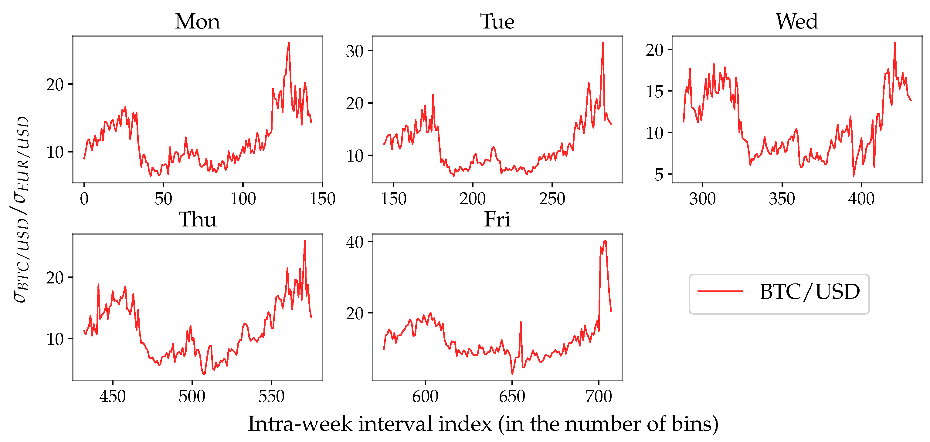
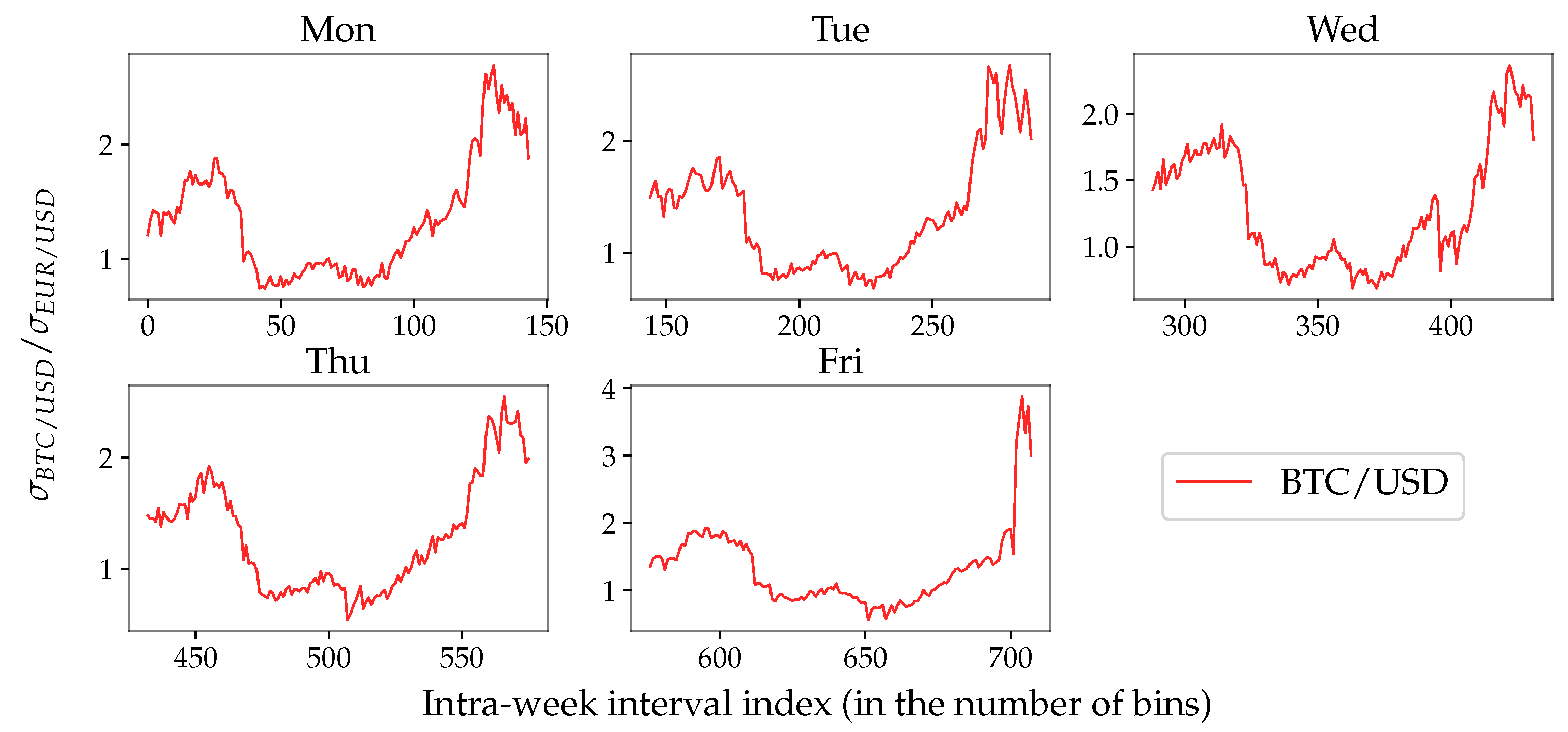
Figure A1.
Daily realised volatility ratio of BTC/USD measured over 10-min time intervals dissecting the entire week into 1008 bins. The volatility is computed according to the “traditional” approach (Equation (20)).
Figure A1.
Daily realised volatility ratio of BTC/USD measured over 10-min time intervals dissecting the entire week into 1008 bins. The volatility is computed according to the “traditional” approach (Equation (20)).

Figure A2.
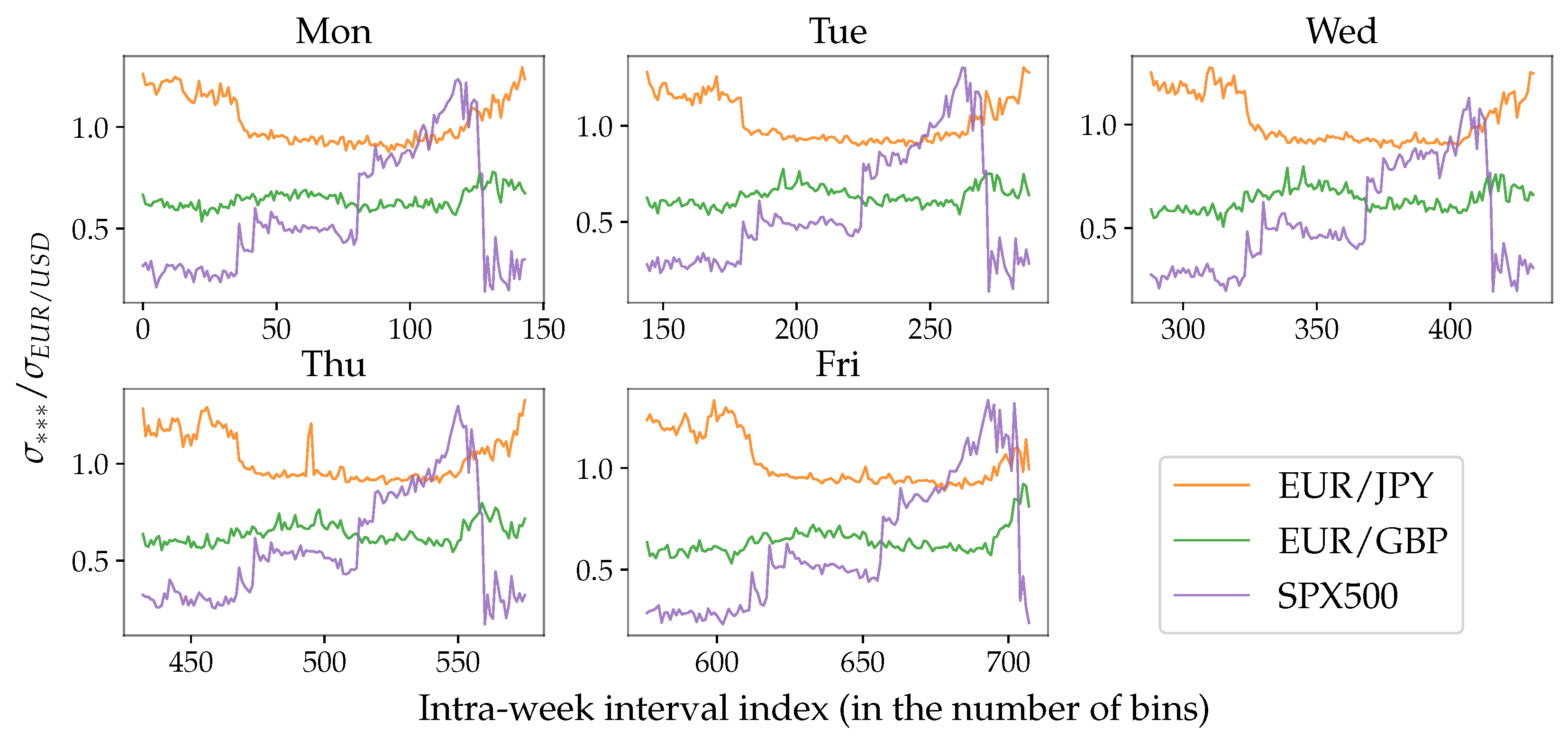
Daily realised volatility ratio of the given exchange rates (labelled by ***) and EUR/USD. The volatility is computed according to the “traditional” approach (Equation (20)).
Figure A2.
Daily realised volatility ratio of the given exchange rates (labelled by ***) and EUR/USD. The volatility is computed according to the “traditional” approach (Equation (20)).
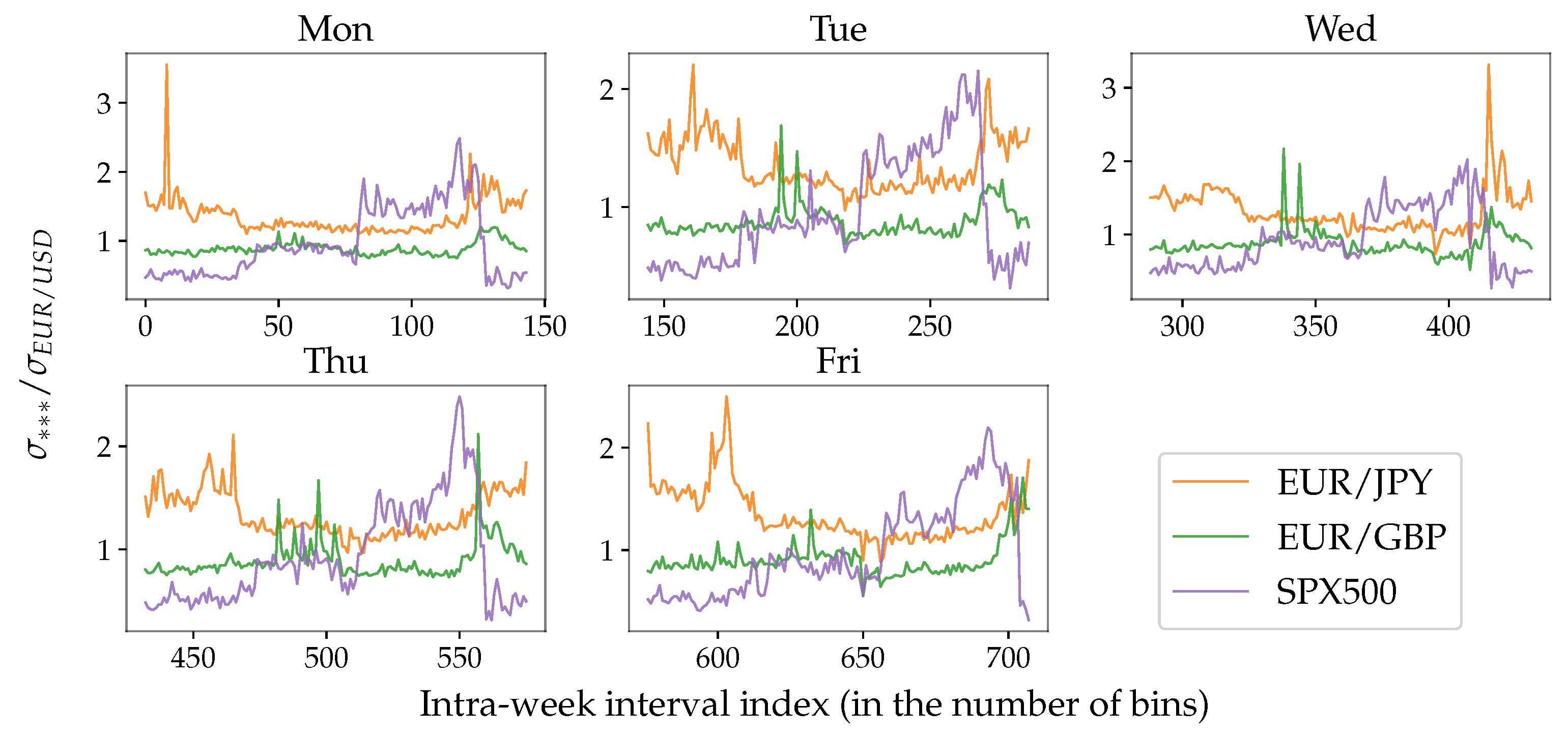
Figure A3.
Daily instantaneous volatility ratio of BTC/USD measured over 10-min time intervals dissecting the entire week into 1008 bins. The volatility is computed according to the novel approach (Equation (19)).
Figure A3.
Daily instantaneous volatility ratio of BTC/USD measured over 10-min time intervals dissecting the entire week into 1008 bins. The volatility is computed according to the novel approach (Equation (19)).

Figure A4.
Daily instantaneous volatility ratio of the given exchange rates (labelled by ***) and EUR/USD. The volatility is computed according to the novel approach (Equation (19)).
Figure A4.
Daily instantaneous volatility ratio of the given exchange rates (labelled by ***) and EUR/USD. The volatility is computed according to the novel approach (Equation (19)).

Table A1.
Daily instantaneous volatility ratio and the weekly standard deviation of two FX (EUR/JPY and EUR/GBP), one crypto (BTC/USD), and one stock (SPX500) exchange rates to EUR/USD. Columns stands for the ratio of the average daily volatility of the corresponding exchange rate and one of EUR/USD. The average value computed over 10-min intervals. Columns contain the standard deviation values of the volatility ratio over the set of 10-min intervals. The subscripts and label the measures made using the traditional volatility estimator (Equation (20)) and the novel approach (Equation (19)) correspondingly. The daily volatility ratios are graphically presented in Figure A2 and Figure A3.
| Monday | EUR/JPY | 1.35 | 0.27 | 1.03 | 0.12 | 1.31 | 2.25 |
| EUR/GBP | 0.89 | 0.1 | 0.64 | 0.04 | 1.39 | 2.50 | |
| BTC/USD | 11.75 | 3.99 | 1.35 | 0.51 | 8.70 | 7.82 | |
| SPX500 | 0.97 | 0.51 | 0.57 | 0.29 | 1.70 | 1.76 | |
| Tuesday | EUR/JPY | 1.35 | 0.23 | 1.02 | 0.11 | 1.32 | 2.09 |
| EUR/GBP | 0.88 | 0.13 | 0.63 | 0.05 | 1.40 | 2.60 | |
| BTC/USD | 11.7 | 4.53 | 1.35 | 0.52 | 8.67 | 8.71 | |
| SPX500 | 0.95 | 0.47 | 0.57 | 0.3 | 1.67 | 1.57 | |
| Wednesday | EUR/JPY | 1.31 | 0.3 | 1.02 | 0.12 | 1.28 | 2.50 |
| EUR/GBP | 0.88 | 0.19 | 0.64 | 0.05 | 1.38 | 3.80 | |
| BTC/USD | 10.83 | 3.74 | 1.29 | 0.46 | 8.40 | 8.13 | |
| SPX500 | 0.93 | 0.42 | 0.53 | 0.26 | 1.75 | 1.62 | |
| Thursday | EUR/JPY | 1.34 | 0.22 | 1.03 | 0.12 | 1.30 | 1.83 |
| EUR/GBP | 0.89 | 0.18 | 0.64 | 0.05 | 1.39 | 3.60 | |
| BTC/USD | 11.42 | 4.42 | 1.29 | 0.5 | 8.85 | 8.84 | |
| SPX500 | 0.93 | 0.49 | 0.57 | 0.28 | 1.63 | 1.75 | |
| Friday | EUR/JPY | 1.35 | 0.28 | 1.03 | 0.12 | 1.31 | 2.33 |
| EUR/GBP | 0.9 | 0.17 | 0.64 | 0.06 | 1.41 | 2.83 | |
| BTC/USD | 11.81 | 4.93 | 1.3 | 0.54 | 9.08 | 9.13 | |
| SPX500 | 0.98 | 0.46 | 0.61 | 0.31 | 1.61 | 1.48 |
References
- Aı, Yacine, and Robert Kimmel. 2007. Maximum likelihood estimation of stochastic volatility models. Journal of Financial Economics 83: 413–52. [Google Scholar]
- Andersen, Torben G., and Jesper Lund. 1997. Estimating continuous-time stochastic volatility models of the short-term interest rate. Journal of Econometrics 77: 343–77. [Google Scholar] [CrossRef]
- Asmussen, Søren, and Hansjörg Albrecher. 2010. Ruin Probabilities. Singapore: World Scientific Publishing Co Pte Ltd. [Google Scholar]
- Bandt, Chstoph, and Faten Shiha. 2007. Order patterns in time series. Journal of Time Series Analysis 28: 646–65. [Google Scholar] [CrossRef]
- Barndorff-Nielsen, Ole E., and Neil Shephard. 2002. Econometric analysis of realized volatility and its use in estimating stochastic volatility models. Journal of the Royal Statistical Society: Series B (Statistical Methodology) 64: 253–80. [Google Scholar] [CrossRef]
- Begušić, Stjepan, Zvonko Kostanjčar, H. Eugene Stanley, and Boris Podobnik. 2018. Scaling properties of extreme price fluctuations in bitcoin markets. Physica A: Statistical Mechanics and Its Applications 510: 400–6. [Google Scholar] [CrossRef]
- Bessembinder, Hendrik. 1994. Bid-ask spreads in the interbank foreign exchange markets. Journal of Financial Economics 35: 317–48. [Google Scholar] [CrossRef]
- BIS. 2016. Triennial Central Bank Survey: Foreign Exchange Turnover in April 2016. Basel: BIS. [Google Scholar]
- Black, Fischer, and Myron Scholes. 1973. The pricing of options and corporate liabilities. Journal of Political Economy 81: 637–54. [Google Scholar] [CrossRef]
- Bollerslev, Tim, and Ian Domowitz. 1993. Trading patterns and prices in the interbank foreign exchange market. The Journal of Finance 48: 1421–43. [Google Scholar] [CrossRef]
- Bollerslev, Tim, and Michael Melvin. 1994. Bid—Ask spreads and volatility in the foreign exchange market: An empirical analysis. Journal of International Economics 36: 355–72. [Google Scholar] [CrossRef]
- Campbell, John Y., Stefano Giglio, Christopher Polk, and Robert Turley. 2018. An intertemporal capm with stochastic volatility. Journal of Financial Economics 128: 207–33. [Google Scholar] [CrossRef]
- Carr, Peter, Hongzhong Zhang, and Olympia Hadjiliadis. 2011. Maximum drawdown insurance. International Journal of Theoretical and Applied Finance 14: 1195–30. [Google Scholar] [CrossRef]
- Chekhlov, Alexei, Stanislav Uryasev, and Michael Zabarankin. 2005. Drawdown measure in portfolio optimization. International Journal of Theoretical and Applied Finance 8: 13–58. [Google Scholar] [CrossRef]
- Cho, D Chinhyung, and Edward W Frees. 1988. Estimating the volatility of discrete stock prices. The Journal of Finance 43: 451–66. [Google Scholar] [CrossRef]
- Cont, Rama. 2001a. Empirical Properties of Asset Returns: Stylized Facts and Statistical Issues. Didcot: Taylor & Francis. [Google Scholar]
- Cont, Rama. 2011b. Statistical modeling of high-frequency financial data. IEEE Signal Processing Magazine 28: 16–25. [Google Scholar] [CrossRef]
- Cotter, John. 2005. Tail behaviour of the euro. Applied Economics 37: 827–40. [Google Scholar] [CrossRef]
- Dacorogna, Michael M., Ulrich A. Müller, Robert J. Nagler, Richard B. Olsen, and Olivier V. Pictet. 1993. A geographical model for the daily and weekly seasonal volatility in the foreign exchange market. Journal of International Money and Finance 12: 413–38. [Google Scholar] [CrossRef]
- Dacorogna, Michel M., Ulrich A. Müller, Olivier V. Pictet, and Casper G. De Vries. 2001. Extremal forex returns in extremely large data sets. Extremes 4: 105–27. [Google Scholar] [CrossRef]
- Dassios, Angelos, and Jia Wei Lim. 2018. An efficient algorithm for simulating the drawdown stopping time and the running maximum of a brownian motion. Methodology and Computing in Applied Probability 20: 189–204. [Google Scholar] [CrossRef]
- De Bondt, Werner F. M., and Richard H. Thaler. 1987. Further evidence on investor overreaction and stock market seasonality. The Journal of Finance 42: 557–81. [Google Scholar] [CrossRef]
- de Vries, Jon Erik, and Halvor Aarhus Aalborg. 2017. What Can Explain the Price, Volatility and Traded Volume of Bitcoin? Master’s dissertation, University of Stavanger, Stavanger, Norway. [Google Scholar]
- Dyhrberg, Anne Haubo. 2016. Bitcoin, gold and the dollar—A garch volatility analysis. Finance Research Letters 16: 85–92. [Google Scholar] [CrossRef]
- Dyhrberg, Anne H., Sean Foley, and Jiri Svec. 2018. How investible is bitcoin? Analyzing the liquidity and transaction costs of bitcoin markets. Economics Letters 171: 140–3. [Google Scholar] [CrossRef]
- Eross, Andrea, Frank Mcgroarty, Andrew Urquhart, and Simon Wolfe. 2017. The Intraday Dynamics of Bitcoin. SSRN Elecronic Journal. Available online: https://dx.doi.org/10.2139/ssrn.3013699 (accessed on 12 September 2018).
- Fang, Lily, Chunmei Lin, and Yuping Shao. 2018. School holidays and stock market seasonality. Financial Management 47: 131–57. [Google Scholar] [CrossRef]
- French, Kenneth R., and Richard Roll. 1986. Stock return variances: The arrival of information and the reaction of traders. Journal of Financial Economics 17: 5–26. [Google Scholar] [CrossRef]
- Gençay, Ramazan, Michel Dacorogna, Ulrich A. Muller, Olivier Pictet, and Richard Olsen. 2001. An Introduction to High-Frequency Finance. Amsterdam: Elsevier. [Google Scholar]
- Glattfelder, James B., Alexandre Dupuis, and Richard B. Olsen. 2011. Patterns in high-frequency fx data: Discovery of 12 empirical scaling laws. Quantitative Finance 11: 599–614. [Google Scholar] [CrossRef]
- Golub, Anton, Gregor Chliamovitch, Alexandre Dupuis, and Bastien Chopard. 2014. Multi-Scale Representation of High Frequency Market Liquidity. Available online: http://dx.doi.org/10.2139/ssrn.2393428 (accessed on 11 September 2018).
- Golub, Anton, James Glattfelder, and Richard B. Olsen. 2017. The Alpha Engine: Designing an Automated Trading Algorithm. Available online: http://dx.doi.org/10.2139/ssrn.2951348 (accessed on 11 September 2018).
- Gottlieb, Gary, and Avner Kalay. 1985. Implications of the discreteness of observed stock prices. The Journal of Finance 40: 135–53. [Google Scholar] [CrossRef]
- Grossman, Sanford J., and Zhongquan Zhou. 1993. Optimal investment strategies for controlling drawdowns. Mathematical Finance 3: 241–76. [Google Scholar] [CrossRef]
- Guillaume, Dominique M., Michel M. Dacorogna, Rakhal R. Davé, Ulrich A. Müller, Richard B. Olsen, and Olivier V. Pictet. 1997. From the bird’s eye to the microscope: A survey of new stylized facts of the intra-daily foreign exchange markets. Finance and Stochastics 1: 95–129. [Google Scholar] [CrossRef]
- Gultekin, Mustafa N., and N. Bulent Gultekin. 1983. Stock market seasonality: International evidence. Journal of Financial Economics 12: 469–81. [Google Scholar] [CrossRef]
- Hadjiliadis, Olympia, and Jan Večeř. 2006. Drawdowns preceding rallies in the brownian motion model. Quantitative Finance 6: 403–9. [Google Scholar] [CrossRef]
- Haferkorn, Martin, and Josué Manuel Quintana Diaz. 2014. Seasonality and interconnectivity within cryptocurrencies-an analysis on the basis of bitcoin, litecoin and namecoin. In International Workshop on Enterprise Applications and Services in the Finance Industry. Cham: Springer, pp. 106–20. [Google Scholar]
- Harris, Larry. 2003. Trading and Exchanges: Market Microstructure for Practitioners. Oxford: Oxford University Press. [Google Scholar]
- Hartmann, Philipp. 1999. Trading volumes and transaction costs in the foreign exchange market: Evidence from daily dollar–yen spot data. Journal of Banking & Finance 23: 801–24. [Google Scholar]
- Hasbrouck, Joel. 2018. High-frequency quoting: Short-term volatility in bids and offers. Journal of Financial and Quantitative Analysis 53: 613–41. [Google Scholar] [CrossRef]
- Ito, Takatoshi, and Yuko Hashimoto. 2006. Intraday seasonality in activities of the foreign exchange markets: Evidence from the electronic broking system. Journal of the Japanese and International Economies 20: 637–64. [Google Scholar] [CrossRef]
- Jondeau, Eric, and Michael Rockinger. 2003. Testing for differences in the tails of stock-market returns. Journal of Empirical Finance 10: 559–81. [Google Scholar] [CrossRef]
- Kaya, Orçun, Jan Schildbach, and Deutsche Bank Ag. 2016. High-frequency trading. Reaching the Limits, Automated Trader Magazine 41: 23–27. [Google Scholar]
- Keim, Donald B. 1983. Size-related anomalies and stock return seasonality: Further empirical evidence. Journal of Financial Economics 12: 13–32. [Google Scholar] [CrossRef]
- Kelly, John L., Jr. 2011. A new interpretation of information rate. In The Kelly Capital Growth Investment Criterion: Theory and Practice. Singapore: World Scientific, pp. 25–34. [Google Scholar]
- Koning, Nico, Daniel T. Cassidy, and Rachid Ouyed. 2018. Extended model of stock price behaviour. Journal of Mathematical Finance 8: 1. [Google Scholar] [CrossRef]
- Landriault, David, Bin Li, and Hongzhong Zhang. 2015. On the frequency of drawdowns for brownian motion processes. Journal of Applied Probability 52: 191–208. [Google Scholar] [CrossRef]
- Liu, Ruiping, Zhichao Shao, Guodong Wei, and Wei Wang. 2017. Garch model with fat-tailed distributions and bitcoin exchange rate returns. Journal of Accounting, Business and Finance Research 1: 71–75. [Google Scholar] [CrossRef]
- Lundberg, Filip. 1909. Uber die theorie der ruck-versicherung. In Trans VI International Congress Actuaries. pp. 877–955. Available online: https://ci.nii.ac.jp/naid/10004541215/ (accessed on 10 December 2018).
- Mancino, Maria Elvira, Maria Cristina Recchioni, and Simona Sanfelici. 2017. Estimation of instantaneous volatility. In Fourier-Malliavin Volatility Estimation. Cham: Springer, pp. 31–47. [Google Scholar]
- Menkhoff, Lukas, Lucio Sarno, Maik Schmeling, and Andreas Schrimpf. 2012. Carry trades and global foreign exchange volatility. The Journal of Finance 67: 681–718. [Google Scholar] [CrossRef]
- Mijatović, Aleksandar, and Martijn R. Pistorius. 2012. On the drawdown of completely asymmetric lévy processes. Stochastic Processes and their Applications 122: 3812–36. [Google Scholar] [CrossRef]
- Müller, Ulrich A., Michel M. Dacorogna, Rakhal D. Davé, Richard B. Olsen, Olivier V. Pictet, and Jacob E. von Weizsäcker. 1997. Volatilities of different time resolutions—Analyzing the dynamics of market components. Journal of Empirical Finance 4: 213–39. [Google Scholar] [CrossRef]
- Müller, Ulrich A., Michel M. Dacorogna, Richard B. Olsen, Olivier V. Pictet, Matthias Schwarz, and Claude Morgenegg. 1990. Statistical study of foreign exchange rates, empirical evidence of a price change scaling law, and intraday analysis. Journal of Banking & Finance 14: 1189–208. [Google Scholar]
- Nakamoto, Satoshi. 2008. Bitcoin: A Peer-to-Peer Electronic Cash System. Available online: http://bitcoin.org/bitcoin.pdf (accessed on 23 October 2018).
- Osborne, Maury F. M. 1959. Brownian motion in the stock market. Operations Research 7: 145–73. [Google Scholar] [CrossRef]
- Ponsford, Matthew P. 2015. A comparative analysis of bitcoin and other decentralised virtual currencies: Legal regulation in the people’s republic of china, canada, and the united states. HKJ Legal Studies 9: 29. [Google Scholar]
- Pospisil, Libor, Jan Vecer, and Olympia Hadjiliadis. 2009. Formulas for stopped diffusion processes with stopping times based on drawdowns and drawups. Stochastic Processes and their Applications 119: 2563–78. [Google Scholar] [CrossRef]
- Rachev, Svetlozar T., Christian Menn, and Frank J. Fabozzi. 2005. Fat-Tailed and Skewed Asset Return Distributions: Implications for Risk Management, Portfolio Selection, and Option Pricing. Hoboken: John Wiley & Sons, vol. 139. [Google Scholar]
- Rolski, Tomasz, Hanspeter Schmidli, Volker Schmidt, and Jozef L. Teugels. 2009. Stochastic Processes for Insurance and Finance. Hoboken: John Wiley & Sons, vol. 505. [Google Scholar]
- Roy, Souvik, and P. Venkateswaran. 2014. Online payment system using steganography and visual cryptography. Paper presented at 2014 IEEE Students’ Conference on Electrical, Electronics and Computer Science, Bhopal, India, March 1–2; Lakes-Bhopal: IEEE, pp. 1–5. [Google Scholar]
- Rozeff, Michael S., and William R. Kinney Jr. 1976. Capital market seasonality: The case of stock returns. Journal of Financial Economics 3: 379–402. [Google Scholar] [CrossRef]
- Sapuric, Svetlana, and Angelika Kokkinaki. 2014. Bitcoin is volatile! Isn’t that right? Paper presented at International Conference on Business Information Systems, Larnaca, Cyprus, May 22–23; Cham: Springer, pp. 255–65. [Google Scholar]
- Schuhmacher, Frank, and Martin Eling. 2011. Sufficient conditions for expected utility to imply drawdown-based performance rankings. Journal of Banking & Finance 35: 2311–18. [Google Scholar]
- Seif, Mostafa, Paul Docherty, and Abul Shamsuddin. 2017. Seasonal anomalies in advanced emerging stock markets. The Quarterly Review of Economics and Finance 66: 169–81. [Google Scholar] [CrossRef]
- Shintate, Takuya, and Lukáš Pichl. 2019. Trend prediction classification for high frequency bitcoin time series with deep learning. Journal of Risk and Financial Management 12: 17. [Google Scholar] [CrossRef]
- Taylor, Howard M. 1975. A stopped brownian motion formula. The Annals of Probability 3: 234–46. [Google Scholar] [CrossRef]
- Zarowin, Paul. 1990. Size, seasonality, and stock market overreaction. Journal of Financial and Quantitative Analysis 25: 113–25. [Google Scholar] [CrossRef]
- Zhang, Hongzhong. 2015. Occupation times, drawdowns, and drawups for one-dimensional regular diffusions. Advances in Applied Probability 47: 210–30. [Google Scholar] [CrossRef]
- Zhang, Hongzhong, and Olympia Hadjiliadis. 2012. Drawdowns and the speed of market crash. Methodology and Computing in Applied Probability 14: 739–52. [Google Scholar] [CrossRef]
| 1. | A basic polynomial functional relationship where a change in input results in a proportional change in output. |
| 2. | A growing list of records containing information on the ownership of all existing Bitcoins. |
| 3. | Information on all cryptocurrencies and trading venues can be found at Coinmarketcap.com. |
| 4. | At the moment of writing the paper, Wall Street and other big financial hubs are considering trading cryptocurrencies, which will potentially result in the higher segregation level. |
| 5. | According to the Bank for International Settlements the daily average FX trading volume in April 2016 was $5.1 trillion (BIS 2016) when the highest registered volume in the crypto market is to the date only $45.8 billion (https://coinmarketcap.com/charts/). |
| 6. | |
| 7. | |
| 8. | |
| 9. | The expression is known in the insurance industry as “adjustment coefficient” or “the Lundberg exponent” (Asmussen and Albrecher 2010). It finds its application in the ruin theory dating back to 1909 (Lundberg 1909). It is also described as the optimal information theoretical betting size called Kelly Criterion (Kelly 2011). |
| 10. | The work Cho and Frees (1988) is particularly interesting due to the analysis the authors did to compare volatilities computed by “natural” and “temporal” estimators. The latter employs time intervals measured between consequent and alternating price moves of fixed relative size and thus is very close to the approach presented in the current paper. |
| 11. | The type of mathematical analysis applied to identify patterns or cycles in a normalised time series data. |
| 12. | It had a minimum at $230 per Bitcoin, temporary maximum at about $20,000, and then a drop to $6000. |
| 13. | The evidence that the distribution of returns approaches the normal one measured over longer timescales. |
| 14. | According to the Table 2. |
Figure 1.
A part of EUR/USD price curve (grey) dissected into a set of directional-changes (grey squares) using a directional-change threshold . The size of the arbitrary chosen threshold is presented in the middle of the figure. Grey circles mark local extremes between two consecutive directional changes. The vertical distance between each directional-change and preceding extreme price is bigger or equal to the size of the threshold . Vertical dashed lines indicate the end of each trend section (identified only after the next event becomes observed) and go through the local extremes (circles). The timeline below the plot contains equal time intervals and length of each directional-change section .

Figure 2.
Heatmaps of the number of directional changes observed by the pair of directional-change thresholds (Y- and X-axis of the plots) in a timeseries of the given length (Geometrical Brownian Motion (GBM), steps in each simulation). Selected trend and volatility values: (a) , ; (b) , ; (c) , . The values on the plots coincide with the ones computed using Equation (17).

Figure 3.
Heat map of the number of directional changes calculated in (a) EUR/USD, (b) BTC/USD, and (c) SPX500 time series. Each point on the grid represents the number of directional changes registered by a unique pair of thresholds . Heatmaps have different scales. Yellow solid lines, specific for each heatmap, label the examples of the areas along which the number of intrinsic events is constant. The dashed lines represent the theoretical areas of the equal number of intrinsic events observed in case of the trend-less time series. White dashed lines are parts of circles centred around the left bottom corner of each picture. The lines go through the intersection of the solid yellow lines and the diagonal of each picture.

Figure 4.
Time of total-move scaling laws computed for BTC/USD, EUR/USD, SPX500, and Geometrical Brownian Motion (GBM). GBM’s parameters are , , , year, and 10 million ticks in total. Scaling parameters C and E correspond to the coefficients of Equation (21).
Figure 4.
Time of total-move scaling laws computed for BTC/USD, EUR/USD, SPX500, and Geometrical Brownian Motion (GBM). GBM’s parameters are , , , year, and 10 million ticks in total. Scaling parameters C and E correspond to the coefficients of Equation (21).

Figure 5.
Instantaneous volatility of three time series generated by GBM with various tick frequencies and fixed volatility (). The volatility is computed by the directional-change approach (Equation (19)). Sizes of the directional change thresholds, used to calculate the volatility values, are put on the X-axis. Red dashed line marks the level.

Figure 6.
Instantaneous volatility seasonality of three Forex (FX) exchange rates computed using the directional-change approach (Equation (19)). Applied directional-change threshold . The whole week is divided by equally spaced time intervals min (1008 bins in total).
Figure 6.
Instantaneous volatility seasonality of three Forex (FX) exchange rates computed using the directional-change approach (Equation (19)). Applied directional-change threshold . The whole week is divided by equally spaced time intervals min (1008 bins in total).

Figure 7.
Realised volatility seasonality patterns of three FX exchange rates computed using the traditional approach (Equation (20)). Time intervals of 1-min have been used to calculate returns. The size of each bin is 10 min, 1008 bins in total.
Figure 7.
Realised volatility seasonality patterns of three FX exchange rates computed using the traditional approach (Equation (20)). Time intervals of 1-min have been used to calculate returns. The size of each bin is 10 min, 1008 bins in total.

Figure 8.
Realised volatility seasonality patterns of BTC/USD and EUR/USD exchange rates computed using the traditional approach (Equation (20)). Time intervals of 1-min have been used to calculate returns. The size of each bin is 10 min, there are 1008 bins in total.
Figure 8.
Realised volatility seasonality patterns of BTC/USD and EUR/USD exchange rates computed using the traditional approach (Equation (20)). Time intervals of 1-min have been used to calculate returns. The size of each bin is 10 min, there are 1008 bins in total.
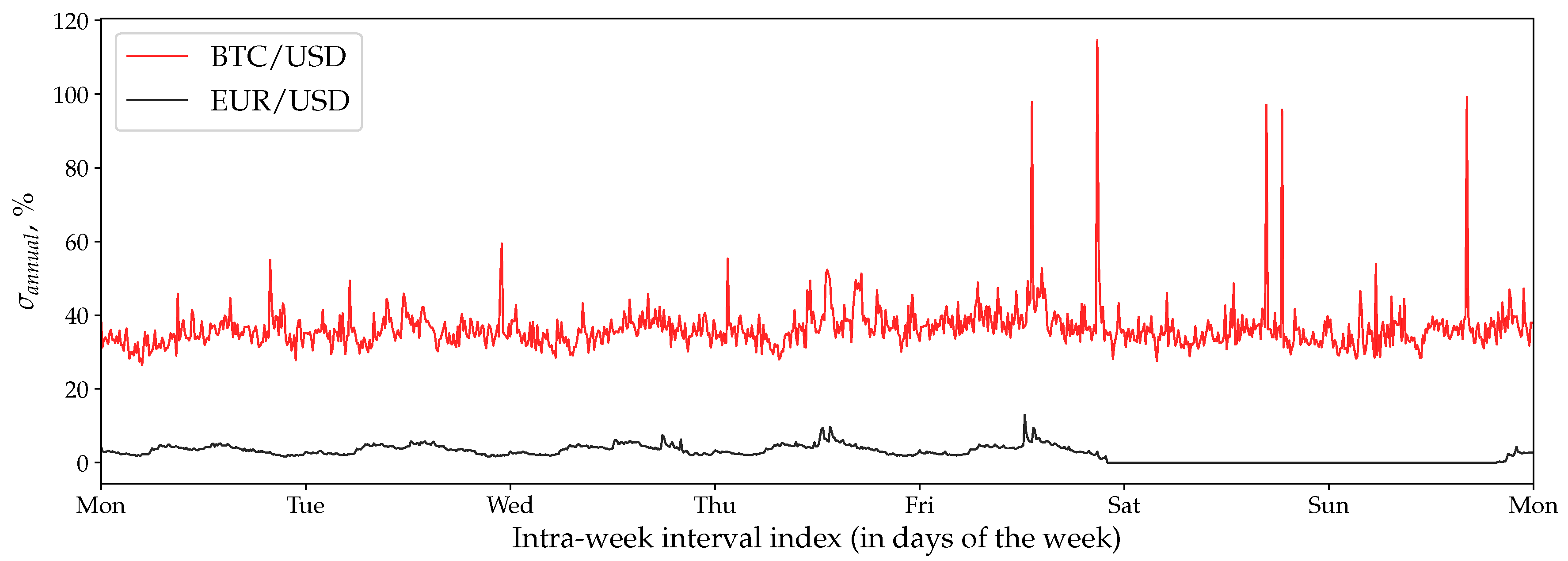
Figure 9.
Instantaneous volatility seasonality of BTC/USD compared to the seasonality pattern of EUR/USD computed using the directional-change approach (Equation (19)). The dark-red curve approximates the Bitcoin seasonality pattern using the Savitzky–Golay filter (number of points in the window is 101, the order of the polynomial is 2). The directional-change threshold was used in both experiments. Each discrete time interval (bin) is min. There are 1008 bins in total.
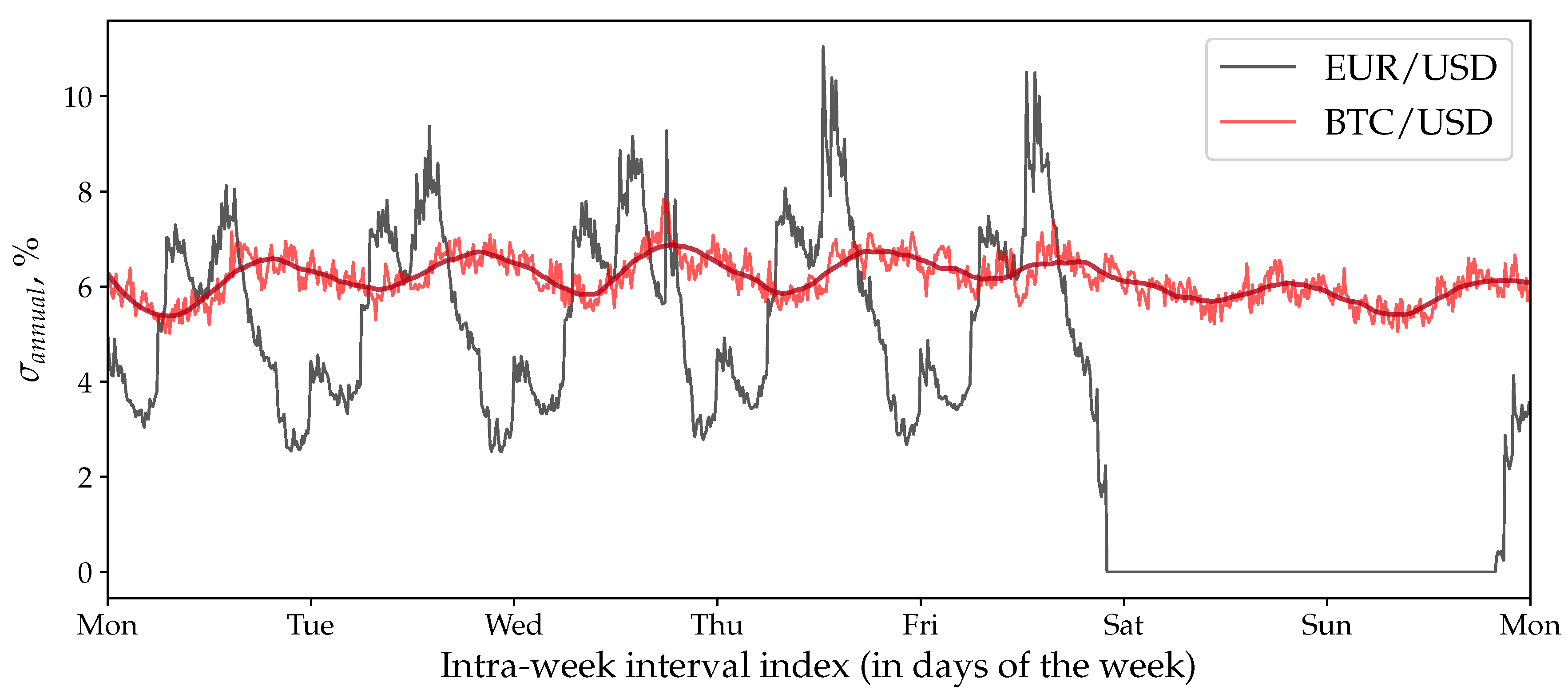
Figure 10.
Volatility seasonality of EUR/USD computed using the novel approach (Equation (19)) and three different thresholds: . The size of a bin is 10 min, there are 1008 bins in a week.
Figure 10.
Volatility seasonality of EUR/USD computed using the novel approach (Equation (19)) and three different thresholds: . The size of a bin is 10 min, there are 1008 bins in a week.

Figure 11.
Volatility seasonality of SPX500 computed using the novel approach (Equation (19)) and three different thresholds: . The size of a bin is 10 min, there are 1008 bins in a week.
Figure 11.
Volatility seasonality of SPX500 computed using the novel approach (Equation (19)) and three different thresholds: . The size of a bin is 10 min, there are 1008 bins in a week.
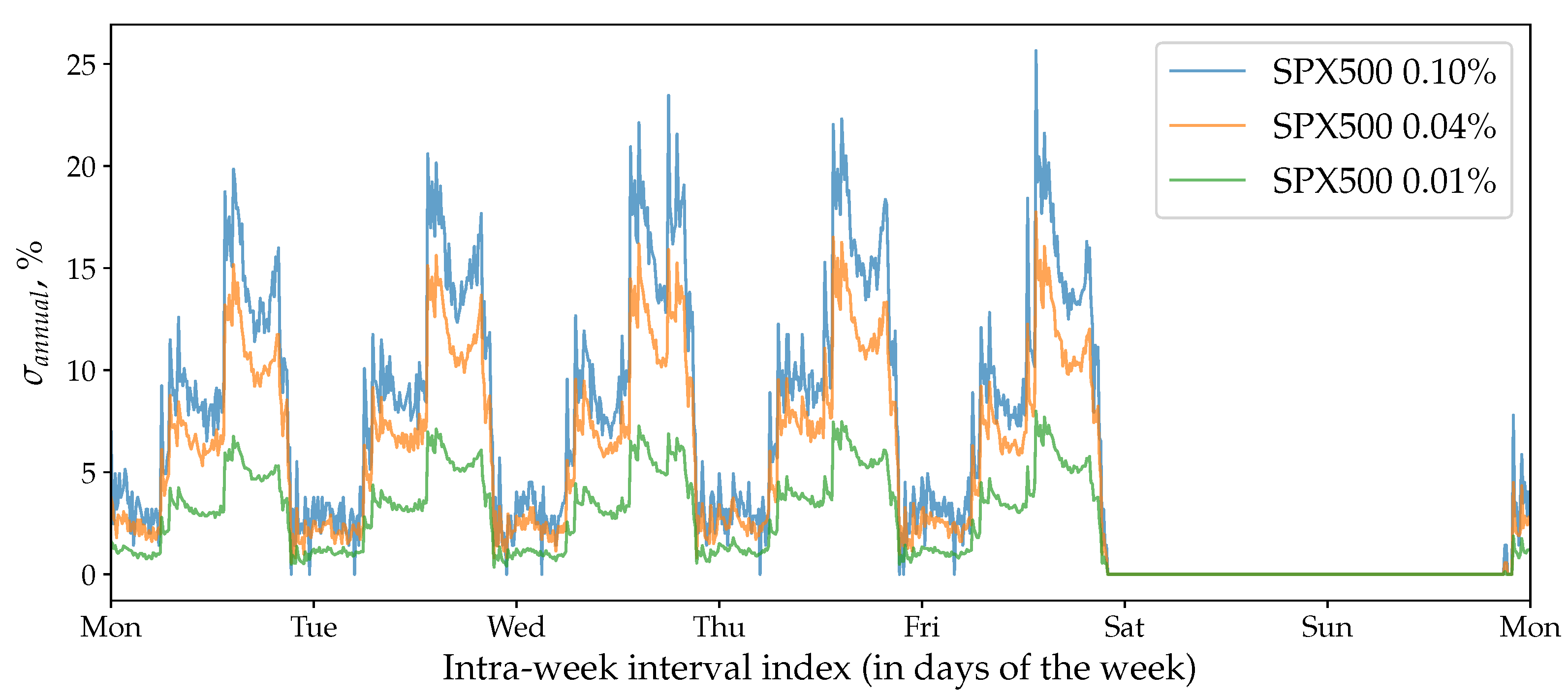
Figure 12.
Instantaneous volatility seasonality of BTC/USD exchange rate computed using the directional-change approach (Equation (19)) and four different thresholds. Applied thresholds, from top to bottom: . The dark solid curves approximate the Bitcoin seasonality patterns using the Savitzky–Golay filter (number of points in the window is 101, order of the polynomial is 2). Bin size min was chosen in all cases (1008 bins in a week). Dashed lines and the numbers over them represent the average level of each seasonality pattern across a week.

Figure 13.
Autocorrelation function of the number of directional changes per 10-min long bins computed in physical time. Vertical dashed lines label weekly intervals. Applied threshold .
Figure 13.
Autocorrelation function of the number of directional changes per 10-min long bins computed in physical time. Vertical dashed lines label weekly intervals. Applied threshold .
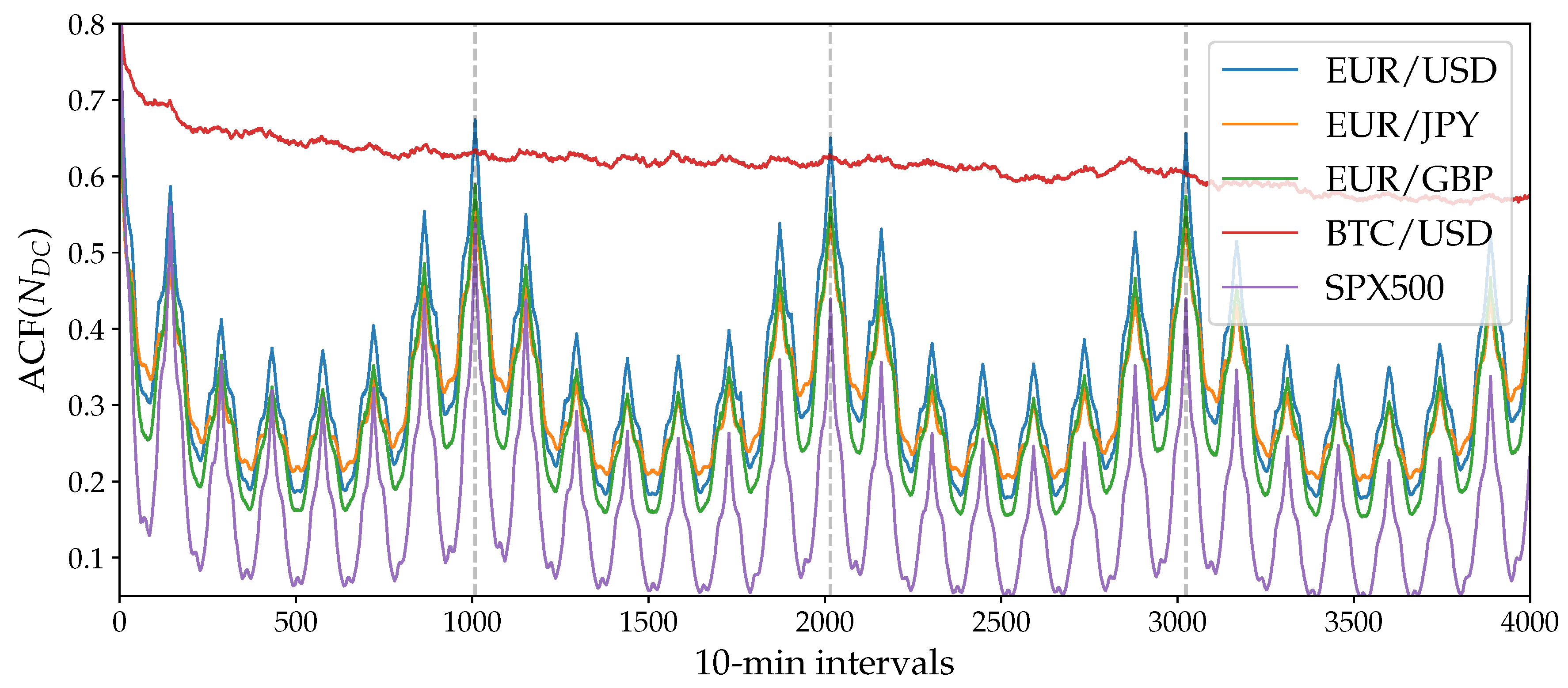
Figure 14.
Autocorrelation function (ACF) of the number of directional changes per a bin in -time. Vertical dashed line labels one week interval. There are 1008 bins in a week.
Figure 14.
Autocorrelation function (ACF) of the number of directional changes per a bin in -time. Vertical dashed line labels one week interval. There are 1008 bins in a week.
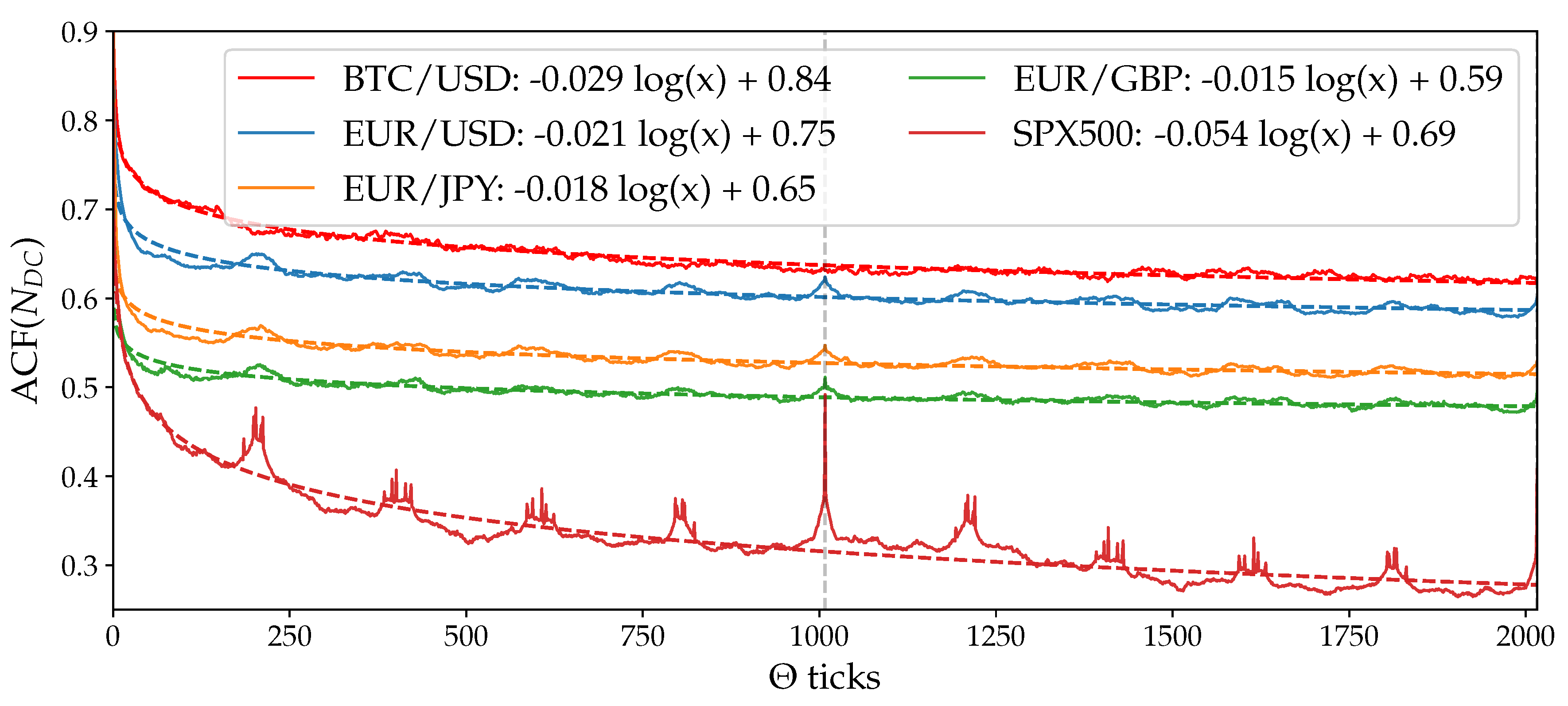
Table 1.
Waiting times and number of directional changes in a Monte Carlo simulation. and are parameters of the Brownian motion used for the test. There are ticks in the simulated time series. , , and are the numbers of directional changes and the average waiting times registered in the Monte Carlo simulation. , , and are theoretical values dictated by Equations (16), (10) and (11) correspondingly. Values and are standard deviations of empirical and theoretical waiting times.
| , % | , % | |||||
|---|---|---|---|---|---|---|
| 1 | 10 | 1.028 | 0.968 | 2.54 × 10⁻⁵ | 1.019 | 2.53 × 10⁻⁶ |
| 20 | 1.009 | 0.989 | 2.78 × 10⁻⁶ | 1.012 | 3.32 × 10⁻⁷ | |
| 30 | 1.001 | 0.995 | 8.79 × 10⁻⁷ | 1.033 | 9.58 × 10⁻⁸ | |
| 6 | 10 | 1.021 | 0.971 | 2.29 × 10⁻⁵ | 1.043 | 2.59 × 10⁻⁶ |
| 20 | 1.005 | 0.993 | 2.94 × 10⁻⁶ | 1.019 | 3.29 × 10⁻⁷ | |
| 30 | 0.987 | 1.011 | 8.84 × 10⁻⁷ | 1.034 | 9.98 × 10⁻⁸ | |
| 11 | 10 | 1.029 | 0.968 | 2.20 × 10⁻⁵ | 1.011 | 2.78 × 10⁻⁶ |
| 20 | 0.994 | 1.006 | 2.72 × 10⁻⁶ | 0.997 | 3.30 × 10⁻⁷ | |
| 30 | 0.986 | 1.014 | 8.82 × 10⁻⁷ | 1.017 | 1.02 × 10⁻⁷ |
Table 2.
Volatility of the considered time series computed using the “traditional” (Equation (20)) and the directional-change (Equation (19)) approaches. Provided values and are the average of four measurements performed with specific parameters: in the “traditional” case time intervals between observations and are 1 min, 10 min, 1 h, and 1 day. In the case of the directional-change intrinsic time approach, the thresholds are , , , (FX prices), , , , (BTC prices), and , , , (SPX500).
| Name | ||||||
|---|---|---|---|---|---|---|
| EUR/USD | 9.72 | 0.03 | 7.53 | 1.38 | 1.29 | 0.02 |
| EUR/JPY | 11.93 | 0.12 | 8.55 | 2.07 | 1.40 | 0.06 |
| EUR/GBP | 8.04 | 0.23 | 5.81 | 1.43 | 1.38 | 0.16 |
| BTC/USD | 84.76 | 8.67 | 80.87 | 22.21 | 1.05 | 0.39 |
| SPX500 | 13.19 | 0.67 | 6.63 | 3.24 | 1.99 | 0.21 |
Table 3.
Parameters of the logarithmic decay used to fit the autocorrelation function (ACF) of the number of directional changes in -time (Figure 14).
Table 3.
Parameters of the logarithmic decay used to fit the autocorrelation function (ACF) of the number of directional changes in -time (Figure 14).
| Name | ||
|---|---|---|
| BTC/USD | −0.029 | 0.84 |
| EUR/USD | −0.021 | 0.75 |
| EUR/JPY | −0.018 | 0.65 |
| EUR/GBP | −0.015 | 0.59 |
| SPX500 | −0.054 | 0.69 |
© 2019 by the authors. Licensee MDPI, Basel, Switzerland. This article is an open access article distributed under the terms and conditions of the Creative Commons Attribution (CC BY) license (http://creativecommons.org/licenses/by/4.0/).
Share and Cite
MDPI and ACS Style
Petrov, V.; Golub, A.; Olsen, R. Instantaneous Volatility Seasonality of High-Frequency Markets in Directional-Change Intrinsic Time. J. Risk Financial Manag. 2019, 12, 54. https://doi.org/10.3390/jrfm12020054
AMA Style
Petrov V, Golub A, Olsen R. Instantaneous Volatility Seasonality of High-Frequency Markets in Directional-Change Intrinsic Time. Journal of Risk and Financial Management. 2019; 12(2):54. https://doi.org/10.3390/jrfm12020054
Chicago/Turabian StylePetrov, Vladimir, Anton Golub, and Richard Olsen. 2019. "Instantaneous Volatility Seasonality of High-Frequency Markets in Directional-Change Intrinsic Time" Journal of Risk and Financial Management 12, no. 2: 54. https://doi.org/10.3390/jrfm12020054