An Analysis of Bitcoin’s Price Dynamics
by
 , ,
, ,
Frode Kjærland
1,2,* ,
,
Aras Khazal
1,
Erlend A. Krogstad
1,
Frans B. G. Nordstrøm
1 and
Are Oust
1 1
NTNU Business School, Norwegian University of Science and Technology, 7491 Trondheim, Norway
2
Nord University Business School, Nord University, 8049 Bodø, Norway
*
Author to whom correspondence should be addressed.
J. Risk Financial Manag. 2018, 11(4), 63; https://doi.org/10.3390/jrfm11040063
Submission received: 20 September 2018
/
Revised: 8 October 2018
/
Accepted: 11 October 2018
/
Published: 15 October 2018
(This article belongs to the Special Issue Alternative Assets and Cryptocurrencies)
Abstract
:This paper aims to enhance the understanding of which factors affect the price development of Bitcoin in order for investors to make sound investment decisions. Previous literature has covered only a small extent of the highly volatile period during the last months of 2017 and the beginning of 2018. To examine the potential price drivers, we use the Autoregressive Distributed Lag and Generalized Autoregressive Conditional Heteroscedasticity approach. Our study identifies the technological factor Hashrate as irrelevant for modeling Bitcoin price dynamics. This irrelevance is due to the underlying code that makes the supply of Bitcoins deterministic, and it stands in contrast to previous literature that has included Hashrate as a crucial independent variable. Moreover, the empirical findings indicate that the price of Bitcoin is affected by returns on the S&P 500 and Google searches, showing consistency with results from previous literature. In contrast to previous literature, we find the CBOE volatility index (VIX), oil, gold, and Bitcoin transaction volume to be insignificant.
1. Introduction
The purpose of this study is to identify the factors that have an impact on the price of Bitcoin. The market value of Bitcoin has grown tremendously in 2017. As the market values of cryptocurrencies grow, it is reasonable to assume that they will start having an effect on certain economies. By estimating the price drivers during the period ranging from 2013 to 2018, this paper will assist investors in making sound investment decisions and aid in the understanding of what drives this phenomenon’s price fluctuations.
Cryptocurrencies are decentralized digital currencies that use encryption to verify transactions. In 2008, Nakamoto (2008) released his paper describing Bitcoin. In January of the following year, Nakamoto released the software that launched the Bitcoin network. As of 2018, Bitcoin is the most commonly known and used cryptocurrency. Since its founding in 2009, the price of Bitcoin has risen from USD 0.07 to an all-time high of USD 20,089 on 17 December 2017 (Quandl.com). At this point in time, its market capitalization was approximately USD 336.4 Billion.
From January 2017 through December, Bitcoin increased by 1270%, and the total cryptocurrency trading volume passed USD 5 billion a day. Interest from the mainstream media, regulators, and the public and financial markets accelerated so much that some call this period Bitcoin’s “IPO moment” (Forbes.com 2017). During 2017, Bitcoin garnered more focus from institutional money, hedge funds, and public funds. Its success culminated with the approval and introduction of Bitcoin derivatives. Due to the exponential rise in attention, we have included two sub-periods to test if the factors have been the same before and after 2017.
We believe that it is important to understand the underlying factors affecting the price of such a highly volatile financial phenomenon. Just as the price of Bitcoins has had an exponential rise in the past year, the academic literature on Bitcoin and cryptocurrencies has experienced a similar increase. Previous literature has used macro-economic, technological, and publicity factors in Bitcoin models (Aalborg et al. 2018; Bouoiyour and Selmi 2016; Ciaian et al. 2016; Garcia et al. 2014; Kristoufek 2013, 2015; Kjærland et al. 2018). However, few academic studies include data that reflect the price fluctuations that Bitcoin experienced in 2017 and 2018. This paper addresses this gap in the literature by assessing what variables drive the price of Bitcoin. As Kristoufek (2015) noted, “because of the dynamic nature of Bitcoin and its rapid price fluctuations, it is logical that the drivers behind the price will vary over time.” Therefore, we have chosen to analyze the drivers yet again.
To estimate the short- and long-term effects of potential price drivers on Bitcoin, an Autoregressive Distributed Lag (ARDL) and Generalized Autoregressive Conditional Heteroscedasticity (GARCH) model is estimated. We find Hashrate to be an irrelevant variable due to the deterministic feature of the Bitcoin supply. The supply of Bitcoins are not dependent on price, as a normal good, but instead the supply of Bitcoins are given by the Bitcoin code and solely dependent on time. Consistent with the previous literature, we find that the S&P 500, Google searches and last week’s return on Bitcoin to be significant explanatory variables, while gold, oil, CBOE volatility index (VIX), and Bitcoin transaction volume are found to be insignificant in the estimation period.
2. Background and Literature Review
2.1. Introduction to Cryptocurrencies and Bitcoin
Several studies focus on the key concepts of cryptocurrencies and particularly Bitcoin (Becker et al. 2013; Brandvold et al. 2015; Dwyer 2015; Nica et al. 2017; Segendorf 2014). According to Dwyer (2015), the major innovation in Bitcoin is its decentralized technology. Instead of storing transactions on a single or set of servers, the database is distributed across a network of participating computers (Böhme et al. 2015). This database is what is called a Blockchain. Blocks are added to the chain in the process of mining Bitcoins. The process of mining revolves around solving complex computational puzzles, and the incentive for miners to participate are transaction fees and Bitcoin rewards. To solve these puzzles, miners need computational power, which is measured by the Hashrate. The Hashrate is the speed at which a computer can complete an operation in the Bitcoin code, while the mining difficulty refers to the level of complexity in the computational puzzles and is directly correlated with the Hashrate. As the Hashrate, either increases or decreases, the underlying Bitcoin algorithm adjusts the mining difficulty so that the supply of Bitcoins follows a predetermined path.1 New coins are generated approximately every 10 min independent of the current price, meaning that the Bitcoin supply is inelastic and time-dependent, as shown in Figure 1. Since the supply is solely dependent on time, we choose to classify the Bitcoin supply as deterministic.
2.2. Literature Review
Several authors have attempted to describe Bitcoin as a currency, stock, or asset. Yermack (2013) argues that Bitcoin appears to behave more similar to a speculative store of value rather than a currency. Dwyer (2015), on the other hand, describes Bitcoin as an electronic currency that can be used to trade and store in a personal balance sheet. Dwyer’s argument is supported by Polasik et al. (2015), who adds that Bitcoin can operate as a medium of exchange alongside other payment technologies.
An increasing number of researchers have focused on the existence of a fundamental value of Bitcoin, and some have studied whether or not it is a bubble. Garcia et al. (2014) finds that Bitcoin is a financial bubble because of the difference between the exchange rate and fundamental value of Bitcoin. He argues for a fundamental value given the cost of mining. Similarly, Hayes (2015, 2018) proposed a specific cost of production model for valuating Bitcoin. Additionally, Cheah and Fry (2015) conclude that Bitcoin is a speculative bubble and that the fundamental value of Bitcoin is zero. Unlike earlier studies, Corbet et al. (2017) found that there is no clear evidence of a bubble in Bitcoin. While these authors discuss if Bitcoin is a bubble or not, Bouri et al. (2017b) found that Bitcoin could be used as an effective diversifier and, in some periods, also display safe-haven and hedge properties.
Some studies have been dedicated to determining the factors that drive the price of Bitcoin. Bouoiyour and Selmi (2015) argue that long-term fundamentals are likely to be major contributors to Bitcoin price variations. Among others, they also found technical factors to be a positive driver of Bitcoin prices (Bouoiyour and Selmi 2015; Ciaian et al. 2016; Garcia et al. 2014; Georgoula et al. 2015; Hayes 2015; Kristoufek 2015). Specifically, Georgoula et al. (2015) and Hayes (2015) found the technical factor Hashrate to be a significant positive price driver. Bouoiyour and Selmi (2016), Garcia et al. (2014), Kristoufek (2015), Kjærland et al. (2018), and Sovbetov (2018) have all used Hashrate as a variable in their respective models.
Other scholars also argue for the significance of fundamental factors such as exchange-trade, equity market indices, currency exchange rates, commodity prices, and transaction volume (Balcilar et al. 2017; Bouri et al. 2018a; Bouoiyour and Selmi 2016; Bouoiyour et al. 2016; Ciaian et al. 2016; Dyhrberg 2016; Kristoufek 2013; Yermack 2013). In contrast to Bouoiyour and Selmi (2015), Polasik et al. (2015) states that an increase in the transaction volume will lead to higher prices and that global economic factors do not seem to be an important driver. Ciaian et al. (2016) also found that supply and demand factors have strong impacts on price and that standard economic currency models can partly explain price fluctuations.
Kristoufek (2013, 2015) analyzed the frequency of online searches on Bitcoin, found them to be a good proxy for interest and popularity, and discovered that the relationship between the price of Bitcoin and online popularity is bidirectional. Ciaian et al. (2016) also found a positive relationship between Wikipedia searches and Bitcoin. Others argue along the same lines as Kristoufek in that it is primarily popularity and investor attractiveness that drive price movements (Bouoiyour et al. 2016).
2.3. Theoretical Foundation
2.3.1. Stock Price Theories and Momentum Theory
Santoni (1987) considers two theories that potentially explain stock prices: the Efficient Market Hypothesis and the Greater Fool theory. The efficient market hypothesis tells us that all relevant information is contained in current stock prices and that prices only change when investors receive new information about fundamentals (Fama 1976). If this theory holds, past price changes contain no useful information about future price changes. The Greater Fool theory says that investors regard fundamental information as irrelevant. An investor buys shares on the belief that some bigger fool will buy them from him at a higher price in the future. This scheme is all about speculation and anticipation of continuing price increases due only to the fact that it has increased in the past.
Momentum in the financial market is an empirically observed trend for rising asset prices to rise further and that decreasing asset prices lead to further decreases. Momentum theory shows that stocks with strong past performance will outperform stocks that have a weak past performance (Jegadeesh and Titman 1993, 2001). This theory relies on short-term movements rather than fundamentals. In financial theory, the cause of momentum is known to be cognitive bias and investors behaving irrationally.2
2.3.2. Volatility
Global financial turmoil impacts economies, assets, and currencies around the world. Financial turmoil also affects the market participants and their investment decisions. During periods of crisis, investors are more inclined to redistribute their investments to assets that are considered to be safe-havens, including currencies. A currency is considered a safe-haven asset if international investors invest in it to minimize losses during periods of financial turmoil. Because of its impact on the development of currency exchange rates, financial turmoil, measured in volatility, is important to include in an exchange rate model.
While there is evidence of negative shocks to equities generating more volatility than positive shocks (Glosten et al. 1993), Baur and McDermott (2012) found that the volatility of gold returns reacts inversely to negative shocks. According to Baur and McDermott (2012), this volatility relation is due to the safe-haven properties of gold. Investors interpret rising gold prices as an increase in macroeconomic uncertainty. Rising uncertainty increases the volatility of gold prices. However, a study by Bouri et al. (2016) find no evidence of an asymmetric return-volatility relation in the Bitcoin market–which in contrast support a safe haven property of Bitcoin. On the other side, Kjærland et al. (2018) have the opposite finding.
3. Research Design
3.1. Data
The dependent variable to be explained by the models is the exchange rate between Bitcoin and the US dollar. The original data are daily spot rates for BTC/USD for the period between 1 January 2013 and 20 February 2018.
To avoid potential issues related to autocorrelation, the daily data are modified into weekly averages. As Bitcoin is traded every day of the week, we filter the data so that only common observations are used. Days when some of the variables have missing values have been removed. The data are gathered from various sources on 21 February 2018. The dependent variable and independent explanatory variables are summarized in Table 1. These are chosen based on previous literature and what we believe affects the price of Bitcoin.
In accordance with the previous literature, we have included the S&P 500 and CBOE Volatility Index (VIX). The S&P 500 is a good indicator of how financial markets are doing, and the VIX is intended to provide an instantaneous measure regarding how much the market believes that the S&P 500 will fluctuate in the next 30 days. By including these two variables, we consider both the numerical returns and risks in the financial markets. Furthermore, we have included the prices of WTI Oil and Gold in our model. Both are considered to be important global commodities whose prices have impacts on almost all economies around the world. These variables are all weekly observations obtained from Thomson Reuters.
To test if publicity and attention given to Bitcoin has an impact on price changes, we include Google Trends. Google search data show normalized weekly statistics that are corrected for trends on searches mentioning the term “Bitcoin” (Google Trends Help 2018) 3. We also test for traditional supply and demand effects by including Bitcoin transaction volume as a variable in this study. Finally, the technological factor Hashrate is included. Volume and Hashrate are weekly data obtained from Quandl.com.
3.2. Descriptive Statistics
3.3. Econometric Method
3.3.1. Autoregressive Distributed Lag Model
According to Im et al. (2003), the ARDL technique is used to estimate short- and long-term relationships between a group of variables by including lags for both the dependent and independent variables. The ARDL model is estimated using ordinary least squares (OLS), where the only difference is the inclusion of lags. As long as the OLS assumptions are fulfilled, the ARDL approach will yield consistent estimates. This procedure is also followed by Ciaian et al. (2016) and Bouri et al. (2018b).
To find the appropriate lag length for each of the underlying variables in the ARDL model, we used the modified Akaike information criteria (AIC), since this criterion is known for having a theoretical advantage over other information criteria (Enders 2009). The model with the lowest AIC and highest R-squared is considered the best. We put in dummy variables for the minimum and maximum observations, in order to tackle the outliers. Using these dummy variables in the regression enhances the reliability of the model (Hansen 2001).
To test for stationarity in a single time series, we use an augmented Dickey–Fuller (ADF) test. If the ADF test shows signs of non-stationarity, the variables can be transformed into first differences, and the test is reapplied. To address possible structural breaks in the time series, we combine the ADF test with a Zivot–Andrews (ZA) test. If structural breaks are identified, the ZA test can be used since it takes structural breaks into account (Vogelsang and Perron 1998).
3.3.2. The Generalized Autoregressive Conditional Heteroscedasticity Model
Regarding the GARCH, in order to control for homoscedasticity, we test the unconditional variance of the regression. Breaking this assumption means that the Gauss–Markov theorem does not hold and that the OLS estimators are not BLUE. Even though the unconditional variance is stable, the conditional variance may not be constant over time. Engle (1982) developed the Autoregressive Conditional Heteroskedasticity (ARCH) model that recognizes the difference between unconditional and conditional variance and lets the conditional variance change over time as a function of previous periods’ error terms. This technique has the ability to capture the effect of volatility clustering, but it requires a model with a relatively long lag structure, which makes estimation difficult. To make this task easier, Bollerslev (1986) proposed the GARCH model that enables a reduction in the number of parameters by imposing nonlinear restrictions. The GARCH model can predict unconditional variance and requires fewer parameters. In a GARCH model, the most recent observations have greater impacts on the predicted volatility.
3.4. Model Estimation
By using OLS, we present three ARDL models. The testing of the models has also been done over different in-sample periods, from 2013, Week 1, to 2016, Week 52, and from 2017, Week 1, to 2018, Week 7. These periods have been chosen to assess the potential changes in what variables affects the price of Bitcoins. The extreme price development in 2017 is also the background for this choice.
Model 1:
Model 2:
Model 3:
A number of post-estimation tests were performed to consider if all the assumptions of OLS are fulfilled. The data set contains of 267 observations. OLS prerequisites were handled by the logarithmic transformation of the data. The post-estimation test results for both the ARDL- and GARCH model can be found in Table A3, Table A4 and Table A5.4
4. Empirical Results
4.1. Main Model (Model 1)
Table 3 and Table 4 present the results of the ARDL and GARCH models. The first model is our main model that includes all variables, while the second model is a reduced version of Model 1 that includes only the significant variables of Model 1 for both the ARDL and GARCH. Table 5 presents the third regression model that includes the variable Hashrate. In the following sections, we will present the results from the main period 2013, Week 1, to 2018, Week 7.
4.1.1. ARDL (1)
As shown in Table 3, the lag of Bitcoin seems to have a significant positive effect on the price of Bitcoin at the 5% level. If last week’s return of Bitcoin is higher by 1%, it is estimated that the return of Bitcoin this week will be higher by 0.19%.
The first difference of S&P 500 is significant at the 5% level and has a positive sign. When the S&P 500 increases by 1%, the price of Bitcoins increases by 1.77%. In contrast, VIX, Oil, Gold, and Volume do not seem to have any significant impact on the price of Bitcoin in the estimated period.
The first difference in the Google Trends variable and its lag are significant at the 1% level. The short-term effects show that, when Google trends increases by 1%, the Bitcoin price is expected to increase by 0.11%. By including the lag of Google, the short-term effect that Google search has on Bitcoin price is 0.22%. Additionally, by including the second lag of Google, which is significant at the 5% level, the total short-term effect that Google search has on Bitcoin price is 0.30%. Lastly, the long-term effect of Google trends on Bitcoin price is 0.37%.5
4.1.2. GARCH (1)
In the GARCH model, the lag of Bitcoin has an almost identical effect as in the ARDL model and is significant at the 1% level. Google and its two lags are significant at the 1% level, which is almost the same as in the ARDL model, although the coefficient for both the first difference and the two lags has decreased. Furthermore, the S&P 500 is found to be insignificant, while it was found significant in the ARDL model. Similar to the ARDL model, VIX, oil, and gold are insignificant. Volume is significant at the 1% level, which is inconsistent with the ARDL model.
The ARCH effects are positive and significant at the 1% level, which indicates that a shock in the variance two weeks ago will have an impact of approximately 56.2% on the volatility in the following week. The GARCH effects are significant at the 5% level. This significance indicates that 31.5% of the volatility last week has an impact on volatility this week. The sum of the ARCH and GARCH effects is approximately 87.7%, which shows the persistence of all volatility and shocks last week, and the impact it has on this week.
4.2. Reduced Model (Model 2)
4.2.1. ARDL (1)
As shown in Table 4, the relationship between the lag and price of Bitcoin is almost the same as in Model 1 and is significant at the 5% level. If the price of Bitcoin last week increased by 1%, the effect is an increase in price this week of 0.19%. Moreover, the S&P 500 seems to have a significant impact on the price of Bitcoin, similar to Model 1. This variable is significant at the 1% level. When the S&P 500 increases by 1%, Bitcoin is estimated to increase by 1.41%.
Google trends has the same significance level as Model 1 and almost equal coefficients. The short-term effect of Google searches is 0.11%, and the total short-term effect is 0.21%. The total long-term effect is 0.34%.
4.2.2. GARCH (1)
The lag of Bitcoin has an almost identical effect as in the ARDL model and is significant at the 1% level. The S&P 500 index is also found to be significant in the GARCH model, just as the ARDL model, but with a slightly lower coefficient.
Google and its two lags are significant at the 5% and 1% levels, respectively, which is almost consistent with the ARDL model. However, the coefficient for both the first difference and the lags has decreased.
The ARCH effects are positive and significant at the 1% level and has an impact of approximately 58.1% on the volatility in the following week. The GARCH effects are positive and significant at the 1% level. About a third (32.4%) of the volatility last week has an impact on the volatility this week. The sum of the ARCH and GARCH effects is approximately 90.5%.
4.3. Model Including Hashrate (Model 3)
The model presented in Table 5 includes the variable Hashrate but is otherwise similar to Model 1. The properties displayed by the variables and their results are also similar to the results of Model 1. However, the first difference of Hashrate has a positive sign in all the estimated periods but is only significant in the third period, from 2017, Week 1, to 2018, Week 7.
4.4. Model Assessment
The weekly log-transformed ARDL models have adjusted R-square values of 29% and 31% for Models 1 and 2, respectively. The ADF test for stationarity indicates that all the variables’ residuals are stationary.6 Other diagnostic tests are run to examine the models’ goodness of fit, and they are fulfilled.7 Lastly, to check for misspecification of the models, a Ramsey RESET test was performed. This test indicates that the models may be misspecified.
5. Discussion and Conclusions
5.1. Discussion
In Model 3, which includes the Hashrate, we observe that the Hashrate has a positive sign in both the estimated period and in-sample periods. The positive sign is contrary to the law of supply and demand, considering that increasing the processing power should in theory lead to an increased supply, which would exert a downward pressure on prices. Due to the deterministic supply of Bitcoins, adding more processing capacity to mining will not lead to an increase in output. However, this variable is only significant in the period from Week 1 of 2017 to Week 7 of 2018, a period of exponential growth in both Bitcoin and Hashrate. Therefore, we believe that the causality between Bitcoin and Hashrate is such that it is the Bitcoin price that drives Hashrate, not the other way around. This outcome is consistent with economic theory since an increase in price will naturally result in the increased profitability of mining. As profitability increases, new actors will enter the mining business, and current miners will increase computational power to the point where excess profits are zero. A price drop will naturally lead to computational power being pulled out of Bitcoin mining. Thus, we consider it irrelevant to include Hashrate as an explanatory variable in a model describing Bitcoin’s price drivers or in calculations of fundamental values of Bitcoin. This outcome is in contrast to previous research that included Hashrate as a variable (Bouoiyour and Selmi 2015; Garcia et al. 2014; Georgoula et al. 2015; Hayes 2015; Kristoufek 2013, 2015; Kjærland et al. 2018; Sovbetov 2018).
The results from the reported regression models indicate that publicity measured in Google Trends has a positive impact on the price of Bitcoin. According to our findings, when people’s curiosity and attention to Bitcoin increase, the demand for Bitcoins also increases. This outcome is consistent with Kristoufek (2013, 2015) and Ciaian et al. (2016), who found that when Google searches on Bitcoin increase, the price of Bitcoin also increases.
We find that the S&P 500 has a positive impact on the price of Bitcoin. This is also the independent variable with the largest coefficient, so it exerts the most influence on the price of Bitcoin in this regression. The interpretation may be as follows: when optimism in financial markets increases, investors also display optimism in Bitcoins. Since risk measured in standard deviation is higher in Bitcoin than that in the S&P 500, Bitcoin investors are likely risk-seeking investors. These findings are also supported by Yermack’s (2013) and Dyhrberg’s (2016) studies in which stock markets have an impact on the price of Bitcoin. Interestingly, Bouri et al. (2018c) find moderate integration between Bitcoin and most of the asset classes studied, included MSCI World and gold.
Our results indicate a positive relationship between the Bitcoin price and its lag, which indicates that the efficient market hypothesis seemingly does not hold. Past returns should be uncorrelated with present returns, and an investment strategy based on past returns should not be profitable. However, it is known that the efficient market hypothesis is widely disputed. Some behavioral economists blame imperfections in financial markets on errors in human reasoning and information processing. Since most investors probably have limited experience with Bitcoins, the context around it is confusing, and there is too much new information to consider in too little time; investors must make quick decisions whether or not to invest. Thus, it is reasonable to assume that investors are affected by the momentum effect of rising prices and vice versa. Observing the price increase last week fuels demand and creates a momentum in price. Combined with Momentum theory, one can think along the lines of the Greater Fool theory in which as the price rapidly increases, investors see get-rich-quick potential by buying now and selling to a greater fool next week.
The estimated regression shows that fear in financial markets, as measured in VIX, does not have a significant impact on the price of Bitcoin. However, in the sub-period between 2017 and 2018, we find a significant negative relationship between VIX and Bitcoin price. During this period, the results indicate that increasing fear of financial turmoil reduces demand for Bitcoins. Since a currency is considered a safe-haven if demand rises during periods of financial stress, the abovementioned results indicate that Bitcoin does not inhibit safe-haven properties, which is inconsistent with the findings of Bouri et al. (2017a, 2017b) and to some extent, with Bouri et al. (2016).
Additionally, both oil and gold were found to be insignificant in the estimated regression period. These findings are in contrast to Kristoufek (2015) and Ciaian et al. (2016), who found that gold and oil have significant positive impacts on Bitcoin prices. This outcome indicates that Bitcoin does not inhibit commodity properties. In addition, the volatility in the price of Bitcoin is unlike any of the two commodities, making it difficult to compare. However, our findings are much in line with the recent study of Bouri et al. (2018b), who find no effects of an aggregate commodity index and gold prices on the price of Bitcoin.
Volume seems to have an insignificant impact on the price of Bitcoin in the estimated period, reflecting Kristoufek’s (2013) findings, which state that the price of Bitcoin cannot be explained by standard economic theory. However, in the GARCH model, volume seems to be a significant variable with a negative sign. The reason may be our use of average daily prices or this outcome may be explained by traditional economic theory regarding supply and demand. When volume increases and demand is met, the price naturally drops, confirming the findings of Ciaian et al. (2016) and Polasik et al. (2015) in which volume exerts an impact on the price of Bitcoin.
In the estimated GARCH model, we find that many of the included variables describe both the return on Bitcoin and volatility. The results of the GARCH model show that the price of Bitcoin is greatly affected by its own historical volatility. The results of the GARCH model are approximately the same as those of the ARDL model, indicating that the ARDL model is robust. Similarly, we observe that our model has approximately the same significant variables during an in-sample period, from Week 1 of 2013 to Week 52 of 2016, the period leading up to the volatile 2017. Although the in-sample period from Week 1 of 2017 to Week 7 of 2018 exhibits different results, it is questionable whether these results are reliable given the low number of observations, the high spike and subsequent fall in price during the period.
5.2. Conclusions
Because of the increase in volatility and the dramatic price fluctuations in 2017, this paper aims to help investors understand the price dynamics of Bitcoin. The results from the empirical analysis provide compelling findings, and the estimated model has strong explanatory power with a high degree of robustness. The primary contribution to Bitcoin research that this study provides is the conclusion that the technological factor Hashrate should not be included in modeling price dynamics or fundamental values since it does not affect Bitcoin supply. Based on our full and reduced model, past price performance, optimism, and Google search volume all play significant roles in explaining Bitcoin prices. When both optimism in financial markets and attention to Bitcoin increase, investors’ willingness to allocate funds to more risky assets, such as Bitcoin, increases. Lastly, we observe that price fluctuations in Bitcoin can be associated with investment theories such as The Greater Fool and Momentum theory.
Appendix A

Table A1.
Results from Adjusted Dickey–Fuller test and Zivot–Andrews on log-transformed variables.
| ADF-Test | Zivot–Andrews | ||||||||
|---|---|---|---|---|---|---|---|---|---|
| Variable | Lag | C, T | t-Statistic | Result | Structural Break | Lag | t-Statistic | Result | |
| BTC | 4 | C, T | −2.095 | I(1) | 2016w26 | 2 | −3.983 | I(1) | |
| Hashrate | 8 | C, T | −3.425 | I(0) | 2013w49 | 4 | −5.142 | ** | I(0) |
| Volume | 10 | C, T | −1.991 | I(1) | 2014w38 | 1 | −6.059 | *** | I(0) |
| S&P 500 | 6 | C, T | −2.043 | I(1) | 2015w34 | 1 | −5.299 | ** | I(0) |
| Gold | 2 | C, T | −2.974 | I(1) | 2016w4 | 2 | −4.748 | I(1) | |
| Oil | 1 | C, T | −1.173 | I(1) | 2014w40 | 1 | −3.767 | I(1) | |
| VIX | 15 | C, T | −2.119 | I(1) | 2015w34 | 0 | −6.133 | *** | I(0) |
| 1 | C, T | −2.481 | I(1) | 2016w25 | 0 | −4.709 | I(1) | ||
Note: ** p < 0.05, *** p < 0.01. All variables are in logarithmic form, C = Constant, T = trend, I(1) = unit root (non-stationarity), and I(0) = no unit root (stationary). The Zivot–Andrews structural break is defined as the lowest (most negative) t-statistic in the ADF test. Structural breaks are allowed for both the incline and the level of trend. The Zivot–Andrews critical values are 1% (−5.57), 5% (−5.08), and 10% (−4.82).
Table A2.
Results from Adjusted Dickey–Fuller test and Zivot–Andrews on the first difference log-transformed variables.
Table A2.
Results from Adjusted Dickey–Fuller test and Zivot–Andrews on the first difference log-transformed variables.
| ADF-Test | Zivot–Andrews | |||||||||
|---|---|---|---|---|---|---|---|---|---|---|
| Variable | Lag | C, T | t-Statistic | Result | Structural Break | Lag | t-Statistic | Result | ||
| BTC | 2 | C, T | −6.899 | *** | I(0) | 2013w50 | 2 | −6.670 | *** | I(0) |
| Hashrate | 9 | C, T | −1.812 | I(1) | 2014w39 | 4 | −6.299 | *** | I(0) | |
| Volume | 15 | C, T | −5.105 | *** | I(0) | 2014w6 | 1 | −11.382 | *** | I(0) |
| S&P 500 | 3 | C, T | −8.091 | *** | I(0) | 2016w7 | 1 | −15.302 | *** | I(0) |
| Gold | 4 | C, T | −7.399 | *** | I(0) | 2014w12 | 2 | −12.356 | *** | I(0) |
| Oil | 7 | C, T | −4.421 | *** | I(0) | 2016w7 | 1 | −12.900 | *** | I(0) |
| VIX | 15 | C, T | −5.267 | *** | I(0) | 2017w17 | 0 | −14.305 | *** | I(0) |
| 1 | C, T | −12.17 | *** | I(0) | 2013w48 | 0 | −18.273 | *** | I(0) | |
Note: *** p < 0.01. All variables are first difference on the logarithmic form; otherwise, see the note to Table A1.
Table A3.
Model 1 assessment.
| ARDL | GARCH | |||||
|---|---|---|---|---|---|---|
| Period | (1) | (2) | (3) | (1) | (2) | (3) |
| Outliers | Yes | Yes | No | Yes | Yes | No |
| Dummies | Yes | Yes | No | Yes | Yes | No |
| Observations | 264 | 205 | 56 | 264 | 205 | 56 |
| R2 | 0.32 | 0.27 | 0.65 | |||
| Adjusted R2 | 0.29 | 0.23 | 0.54 | |||
| AIC | −483.83 | −359.30 | −117.63 | −545.39 | −432.77 | −548.31 |
| Ramsey RESET, p-value | 0.0000 | 0.0000 | 0.911 | |||
| Durbin–Watson | 2.07 | 2.13 | 2.01 | |||
| Ljung-Box Q Stat | 0.4265 | 0.5193 | 0.5088 | |||
| ADF, residual value | 0.0002 | 0.0017 | 0.0000 | 0.0000 | 0.0004 | 0.0000 |
Note: (1) = 2013w1–2018w7, (2) = 2013w1–2016w52, and (3) = 2017w1–2018w7.
Table A4.
Model 2 assessment.
| ARDL | GARCH | |||||
|---|---|---|---|---|---|---|
| Period | (1) | (2) | (3) | (1) | (2) | (3) |
| Outliers | Yes | Yes | No | Yes | Yes | No |
| Dummies | Yes | Yes | No | Yes | Yes | No |
| Observations | 264 | 205 | 56 | 264 | 205 | 56 |
| R2 | 0.31 | 0.25 | 0.56 | |||
| Adjusted R2 | 0.29 | 0.23 | 0.50 | |||
| AIC | −489.41 | −366.10 | −117.35 | −552.80 | −442.78 | −554.30 |
| Ramsey RESET, p-value | 0.0000 | 0.0000 | 0.765 | |||
| Durbin–Watson | 2.08 | 2.14 | 1.85 | |||
| Ljung-Box Q Stat | 0.4155 | 0.5127 | 0.5041 | |||
| ADF, residual value | 0.0003 | 0.0024 | 0.0008 | 0.0000 | 0.0005 | 0.0000 |
Note: (1) = 2013w1–2018w7, (2) = 2013w1–2016w52, and (3) = 2017w1–2018w7.
Table A5.
Model 3 assessment.
| ARDL | GARCH | |||||
|---|---|---|---|---|---|---|
| Period | (1) | (2) | (3) | (1) | (2) | (3) |
| Outliers | Yes | Yes | No | Yes | Yes | No |
| Dummies | Yes | Yes | No | Yes | Yes | No |
| Observations | 264 | 205 | 56 | 264 | 205 | 56 |
| R2 | 0.33 | 0.27 | 0.68 | |||
| Adjusted R2 | 0.29 | 0.22 | 0.57 | |||
| AIC | −482.70 | −357.37 | −120.47 | −543.71 | −430.78 | −548.59 |
| Ramsey RESET, p-value | 0.0000 | 0.0000 | 0.817 | |||
| Durbin–Watson | 2.06 | 2.13 | 1.87 | |||
| Ljung-Box Q Stat | 0.4265 | 0.5187 | 0.5075 | |||
| ADF, residual value | 0.0001 | 0.0014 | 0.0004 | 0.0000 | 0.0005 | 0.0000 |
Note: (1) = 2013w1–2018w7, (2) = 2013w1–2016w52, and (3) = 2017w1–2018w7.
Table A6.
Results of the variance inflation factors: test for autocorrelation.
| Model 1 | Model 2 | Model 3 | |||
|---|---|---|---|---|---|
| Variable | VIF-Value | Variable | VIF-Value | Variable | VIF-Value |
| 1.29 | 1.26 | 1.29 | |||
| 1.11 | 1.04 | 1.11 | |||
| 4 | 1.09 | 4.01 | |||
| 1.24 | 1.17 | 1.24 | |||
| 1.15 | 1.16 | 1.16 | |||
| 4.03 | 4.06 | ||||
| 1.13 | 1.14 | ||||
| 1.25 | 1.25 | ||||
| 1.18 | 1.18 | ||||
| 1.02 | |||||
References
- Aalborg, Halvor Aarhus, Peter Molnár, and Jon Erik de Vries. 2018. What can explain the price, volatility and trading volume of Bitcoin? Finance Research Letters. forthcoming. [Google Scholar] [CrossRef]
- Balcilar, Mehmet, Elie Bouri, Rangan Gupta, and David Roubaud. 2017. Can volume predict Bitcoin returns and volatility? A quantiles-based approach. Economic Modelling 64: 74–81. [Google Scholar] [CrossRef]
- Baur, Dirk G., and Thomas K.J. McDermott. 2012. Safe haven assets and investor behavior under uncertainty. Institute for International Integration Studies. Available online: https://rbnz.govt.nz/-/media/ReserveBank/Files/Publications/Seminars%20and%20workshops/feb2012/4682207.pdf (accessed on 14 January 2018).
- Becker, Jörg, Dominic Breuker, Tobias Heide, Justus Holler, Hans Peter Rauer, and Rainer Böhme. 2013. Can We Afford Integrity by Proof-of-Work? Scenarios Inspired by the Bitcoin Currency. In The Economics of Information Security and Privacy. Berlin and Heidelberg: Springer Heidelberg, pp. 135–56. [Google Scholar]
- Böhme, Rainer, Nicolas Christin, Benjamin Edelman, and Tyler Moore. 2015. Bitcoin: Economics, Technology, and Governance. Journal of Economic Perspectives 29: 213–38. [Google Scholar] [CrossRef]
- Bollerslev, Tim. 1986. Generalized autoregressive conditional heteroskedasticity. Journal of Econometrics 31: 307–27. [Google Scholar] [CrossRef]
- Bouoiyour, Jamal, and Refk Selmi. 2015. What Does Bitcoin Look Like? Annals of Economics and Finance 16: 449–92. [Google Scholar]
- Bouoiyour, Jamal, and Refk Selmi. 2016. Bitcoin: A beginning of a new phase? Economics Bulletin 36: 1430–40. [Google Scholar]
- Bouoiyour, Jamal, Refk Selmi, Aviral Kumar Tiwari, and Olaolu Richard Olayeni. 2016. What drives Bitcoin price? Economics Bulletin 36: 843–50. [Google Scholar]
- Bouri, Elie, Georges Azzi, and Anne Haubo Dyhrberg. 2016. On the Return-Volatility Relationship in the Bitcoin Market around the Price Crash of 2013. Available online: https://ssrn.com/abstract=2869855 or http://dx.doi.org/10.2139/ssrn.2869855 (accessed on 5 February 2018).[Green Version]
- Bouri, Elie, Naji Jalkh, Peter Molnár, and David Roubaud. 2017a. Bitcoin for energy commodities before and after the December 2013 crash: Diversifier, hedge or safe haven? In Applied Economics. vol. 49, pp. 5063–73. [Google Scholar] [CrossRef]
- Bouri, Elie, Peter Molnár, Georges Azzi, David Roubaud, and Lars Ivar Hagfors. 2017b. On the hedge and safe haven properties of Bitcoin: Is it really more than a diversifier? Finance Research Letters 20: 192–8. [Google Scholar] [CrossRef]
- Bouri, Elie, Chi Keung Marco Lau, Brian Lucey, and David Roubaud. 2018a. Trading volume and the predictability of return and volatility in the cryptocurrency market. In Finance Research Letters. forthcoming. [Google Scholar] [CrossRef]
- Bouri, Elie, Rangan Gupta, Amine Lahiani, and Muhammad Shahbaz. 2018b. Testing for asymmetric nonlinear short- and long-run relationships between bitcoin, aggregate commodity and gold prices. Resources Policy 57: 224–35. [Google Scholar] [CrossRef]
- Bouri, Elie, Mahamitra Das, Rangan Gupta, and David Roubaud. 2018c. Spillovers between Bitcoin and other assets during bear and bull markets. Applied Economics 50: 5935–49. [Google Scholar] [CrossRef]
- Brandvold, Morten, Peter Molnár, Kristian Vagstad, and Ole Christian Andreas Valstad. 2015. Price discovery on Bitcoin exchanges. Journal of International Financial Markets, Institutions and Money 36: 18–35. [Google Scholar] [CrossRef]
- Cheah, Eng-Tuck, and John Fry. 2015. Speculative bubbles in Bitcoin markets? An empirical investigation into the fundamental value of Bitcoin. Economics Letters 130: 32–36. [Google Scholar] [CrossRef] [Green Version]
- Ciaian, Pavel, Miroslava Rajcaniova, and d’Artis Kancs. 2016. The economics of BitCoin price formation. Applied Economics 48: 1799–815. [Google Scholar] [CrossRef]
- Corbet, Shaen, Brian Lucey, and Larisa Yarovaya. 2017. Datestamping the Bitcoin and Ethereum bubbles. Finance Research Letters 26: 81–88. [Google Scholar] [CrossRef]
- Dwyer, Gerald P. 2015. The economics of Bitcoin and similar private digital currencies. Journal of Financial Stability 17: 81–91. [Google Scholar] [CrossRef] [Green Version]
- Dyhrberg, Anne Haubo. 2016. Bitcoin, gold and the dollar—A GARCH volatility analysis. Finance Research Letters 16: 85–92. [Google Scholar] [CrossRef]
- Enders, Walter. 2009. Applied Economic Time Series, 3rd ed. Hoboken: John Wiley & Sons. [Google Scholar]
- Engle, Robert F. 1982. Autoregressive conditional heteroscedasticity with estimates of the variance of United Kingdom inflation. Econometrica: Journal of the Econometric Society 50: 987–1007. [Google Scholar] [CrossRef]
- Fama, Eugene F. 1976. Efficient capital markets: Reply. The Journal of Finance 31: 143–45. [Google Scholar] [CrossRef]
- Garcia, David, Claudio J. Tessone, Pavlin Mavrodiev, and Nicolas Perony. 2014. The digital traces of bubbles: Feedback cycles between socio-economics signals in the Bitcoin economy. Journal of the Royal Society Interface 11: 1–28. [Google Scholar] [CrossRef] [PubMed]
- Georgoula, Ifigeneia, Demitrios Pournarakis, Christos Bilanakos, Dionisios Sotiropoulos, and George M. Giaglis. 2015. Using Time-Series and Sentiment Analysis to Detect the Determinants of Bitcoin Prices. Available online: http://ssrn.com/abstract=2607167 (accessed on 30 January 2018).
- Glosten, Lawrence R., Ravi Jagannathan, and David E. Runkle. 1993. On the relation between the expected value and the volatility of the nominal excess return on stocks. The Journal of Finance 48: 1779–801. [Google Scholar] [CrossRef]
- Google Trends Help. 2018. Available online: https://support.google.com/trends/?hl=en#topic=6248052 (accessed on 15 February 2018).
- Hansen, Bruce E. 2001. The New Econometrics of Structural Change: Dating Breaks in U.S. Labour Productivity. Journal of Economic Perspectives 15: 117–28. [Google Scholar] [CrossRef]
- Hayes, Adam S. 2015. Cryptocurrency value formation: An empirical study leading to a cost of production model for valuing bitcoin. Telematics and Informatics 34: 1308–21. [Google Scholar] [CrossRef]
- Hayes, Adam S. 2018. Bitcoin price and its marginal cost of production: Support for a fundamental value. Applied Economics Letters 5: 1–7. [Google Scholar] [CrossRef]
- Im, Kyung So, M. Hashem Pesaran, and Yongcheol Shin. 2003. Testing for unit roots in heterogeneous panels. Journal of Econometrics 115: 53–74. [Google Scholar] [CrossRef]
- Jegadeesh, Narasimhan, and Sheridan Titman. 1993. Returns to Buying Winners and Selling Losers: Implications for Stock Market Efficiency. The Journal of Finance 48: 65–91. [Google Scholar] [CrossRef] [Green Version]
- Jegadeesh, Narasimhan, and Sheridan Titman. 2001. Profitability of momentum strategies: An evaluation of alternative explanations. The Journal of Finance 56: 699–720. [Google Scholar] [CrossRef]
- Kjærland, Frode, Maria Meland, Are Oust, and Vilde Øyen. 2018. How can Bitcoin Price Fluctuations be Explained? International Journal of Economics and Financial Issues 8: 323–32. [Google Scholar]
- Kristoufek, Ladislav. 2013. BitCoin meets Google Trends and Wikipedia: Quantifying the relationship between phenomena of the Internet era. Scientific Reports 3: 3415. [Google Scholar] [CrossRef] [PubMed] [Green Version]
- Kristoufek, Ladislav. 2015. What Are the Main Drivers of the Bitcoin Price? Evidence from Wavelet Coherence Analysis. PLoS ONE 10: e0123923. [Google Scholar] [CrossRef] [PubMed]
- Nakamoto, Satoshi. 2008. Bitcoin: A Peer-to-Peer Electronic Cash System. Available online: http://bitcoin.org/bitcoin.pdf (accessed on 9 January 2018).
- Nica, Octavian, Karolina Piotrowska, and Klaus Reiner Schenk-Hoppé. 2017. Cryptocurrencies: Economic Benefits and Risks. FinTech Working Paper. Manchester: University of Manchester, Available online: https://ssrn.com/abstract=3059856 (accessed on 10 March 2018).
- Polasik, Michal, Anna Iwona Piotrowska, Tomasz Piotr Wisniewski, Radoslaw Kotkowski, and Geoffrey Lightfoot. 2015. Price Fluctuations and the Use of Bitcoin: An Empirical Inquiry. International Journal of Electronic Commerce 20: 9–49. [Google Scholar] [CrossRef] [Green Version]
- Santoni, Gary J. 1987. The great bull markets 1924–29 and 1982–87: Speculative bubbles or economic fundamentals? Federal Reserve Bank of St. Louis Review 69: 16–29. [Google Scholar] [CrossRef]
- Segendorf, Björn. 2014. What is bitcoin? Sveriges Riksbank Economic Review 2: 71–87. [Google Scholar]
- Sovbetov, Yhlas. 2018. Factors Influencing Cryptocurrency Prices: Evidence from Bitcoin, Ethereum, Dash, Litcoin, and Monero. Journal of Economics and Financial Analysis 2: 1–27. [Google Scholar]
- Vogelsang, Timothy J., and Pierre Perron. 1998. Additional Tests for a Unit Root Allowing for a Break in the Trend Function at an Unknown Time. International Economic Review 39: 1073–100. [Google Scholar] [CrossRef]
- Yermack, David. 2013. Is Bitcoin a Real Currency? An economic appraisal. National Bureau of Economic Research Working Paper Series No. 19747. Available online: http://www.nber.org/papers/w19747 (accessed on 18 January 2018).
| 1. | Bitcoin rewards are currently at 12.5 coins per block, but the protocol requires that the reward is halved every 210,000 mined blocks. Mining 210,000 blocks takes approximately four years. Given the current level of network processing power, the next halving will take place around early June 2020, bringing the mining reward down to 6.25 coins. |
| 2. | Cognitive biases are errors in thinking that affect the decisions and judgments that people make. |
| 3. | Google does not differentiate between the upper- and lowercase letters, meaning that searches made on “Bitcoin” or “bitcoin” are considered the same. |
| 4. | The following post-estimation tests have been conducted for OLS-assumptions: Ramsey RESET test, Durbin–Watson, Variance Inflation Factors (VIF), and Adjusted Dickey–Fuller. For GARCH: Ljung Box Q-statistics. |
| 5. | The long-term effect of a variable is calculated in following way: ßt + ßt−1 + ... + ßt−n/(1 − ß1∆lnBTCt−1). |
| 6. | |
| 7. |
Figure 1.
Bitcoin deterministic supply.
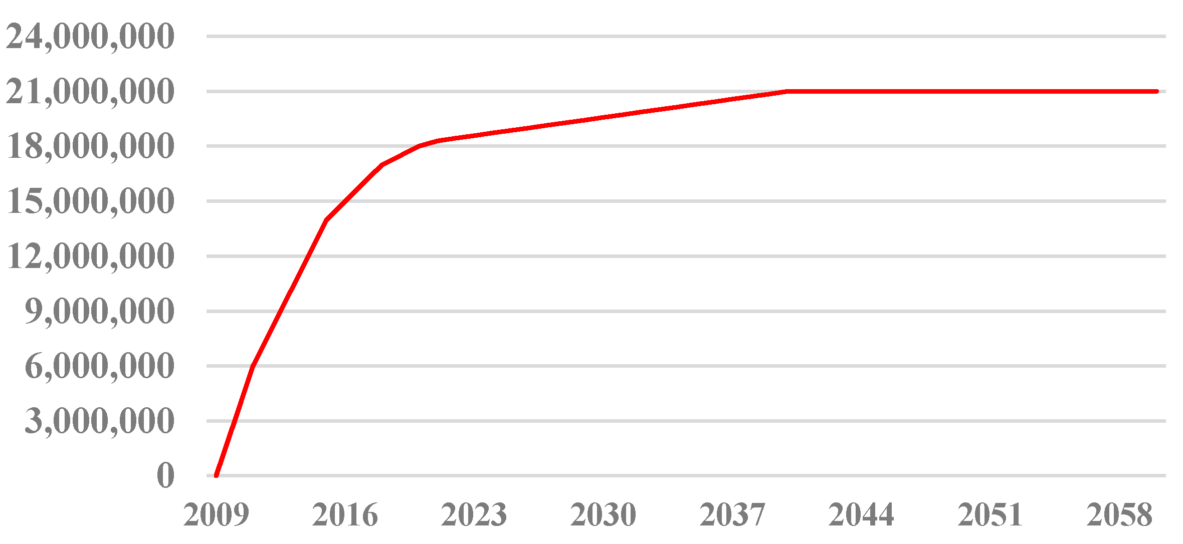
Figure 2.
Bitcoin Market Price (USD), Quandl.

Figure 3.
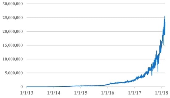
Bitcoin Hashrate, Quandl.

Figure 4.
Bitcoin Transaction Volume, Quandl.

Figure 5.
S&P 500 Index, Thomson Reuters.
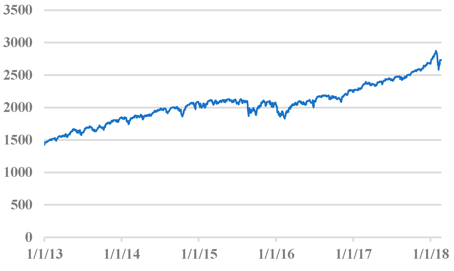
Figure 6.
Gold Index (USD), Thomson Reuters.
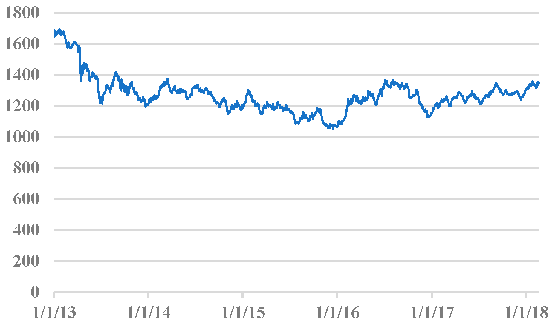
Figure 7.
Crude Oil-WTI Spot, Thomson Reuters.

Figure 8.
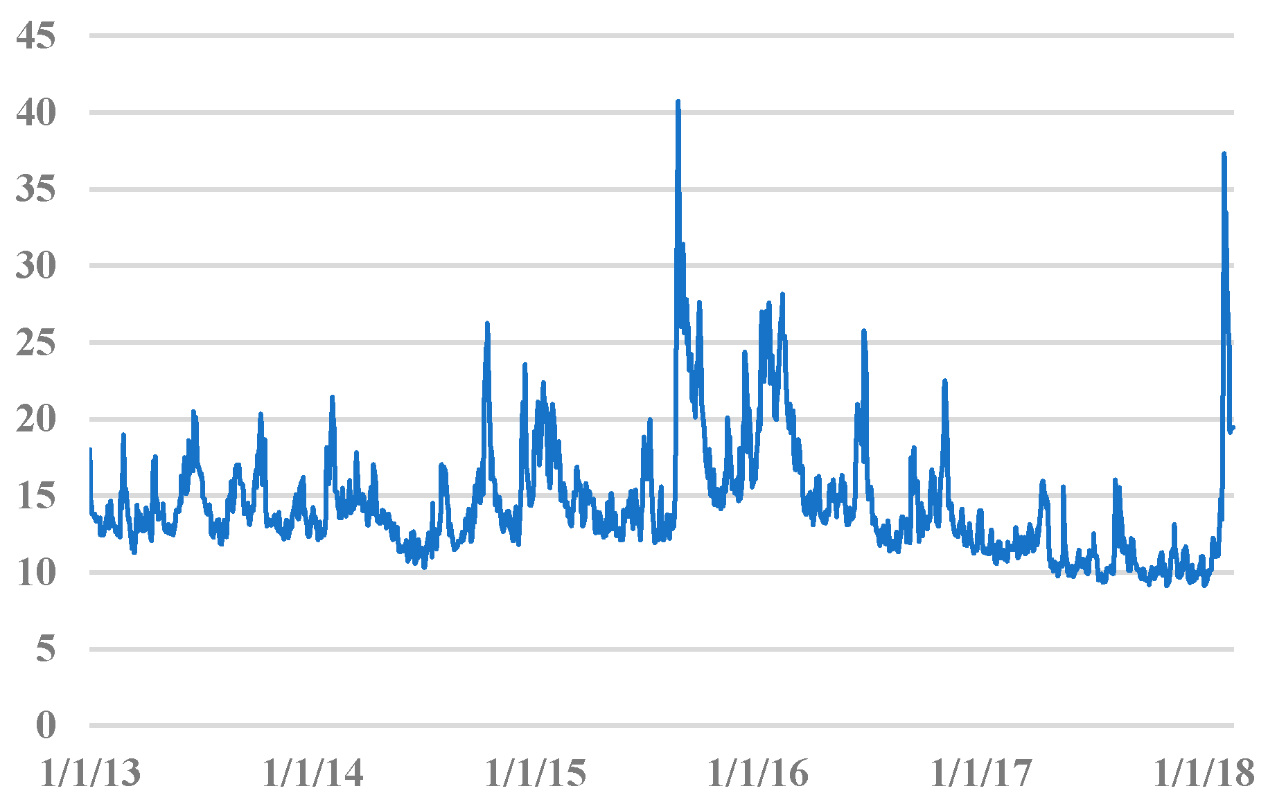
CBOE Volatility Index, Thomson Reuters.

Figure 9.
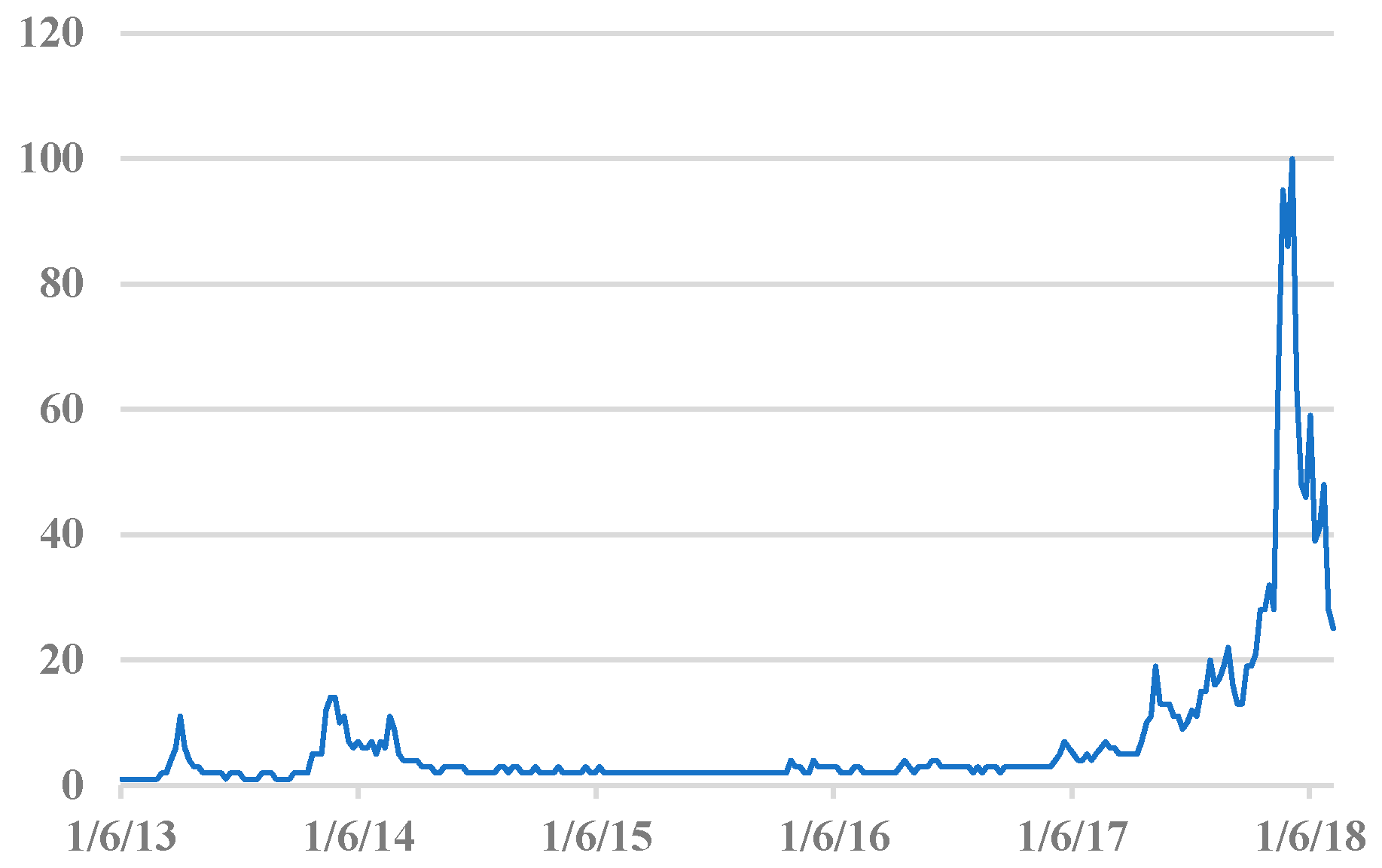
Google Search “Bitcoin,” Google Trends.

Table 1.
Variable Overview.
| Variable | Description | Source |
|---|---|---|
| BTC | exchange rate between Bitcoin and the US Dollar | Quandl |
| Hashrate | the estimated number of giga hashes per second the Bitcoin network is performing | Quandl |
| Volume | total output volume of Bitcoin | Quandl |
| S&P 500 | S&P 500 is an index of the 500 largest US listed Corporations | Thomson Reuters Eikon |
| Gold | Goldman Sachs Commodity Index Gold | Thomson Reuters Eikon |
| Oil | WTI Crude Oil Spot Price in USD per barrel | Thomson Reuters Eikon |
| VIX | implicit volatility of options on the S&P 500, a measure of the expected market volatility the next 30 days | Thomson Reuters Eikon |
| normalized weekly statistics on the search term “Bitcoin”, corrected for trends | Google Trend |
Table 2.
Descriptive statistics.
| Variable | Obs. | Mean | Std. Dev. | Min. | Max. |
|---|---|---|---|---|---|
| BTC | 267 | 1372.9 | 2836.016 | 13.47221 | 17,612.51 |
| Hashrate | 267 | 2,132,903 | 3,936,302 | 20.80583 | 2.26 × 10⁷ |
| Volume | 267 | 238,664.5 | 85,023.81 | 73,429.4 | 558,364.4 |
| S&P 500 | 267 | 2053.9 | 296.3 | 1462.5 | 2844.4 |
| Gold | 267 | 1270.8 | 114.3 | 1063.0 | 1685.2 |
| Oil | 267 | 66.7 | 24.7 | 28.5 | 108.9 |
| VIX | 267 | 14.4 | 3.6 | 9.3 | 31.5 |
| 267 | 7.3 | 13.4 | 1 | 100 |
Table 3.
Results of ARDL & GARCH models (Model 1).
| ARDL | GARCH | |||||
|---|---|---|---|---|---|---|
| Time Period | (1) | (2) | (3) | (1) | (2) | (3) |
| 0.19 (2.23) ** | 0.222 (2.14) ** | 0.206 (1.04) | 0.225 (5.43) *** | 0.329 (6.44) *** | 0.293 (4.98) *** | |
| −0.042 (1.41) | −0.027 (0.79) | −0.134 (2.33) ** | −0.046 (2.61) *** | −0.022 (1.26) | −0.15 (0.62) | |
| 1.772 (2.16) ** | 2.55 (2.69) *** | −1.707 (1.04) | 1.038 (1.59) | 1.272 (1.85) * | 1.318 (1.90) * | |
| −0.072 (0.50) | −0.075 (0.47) | −0.141 (0.40) | −0.001 (0.00) | 0.021 (0.17) | 0.005 (0.04) | |
| 0.142 (0.95) | 0.147 (0.87) | 0.341 (0.77) | 0.023 (0.18) | 0.027 (0.22) | 0.005 (0.04) | |
| 0.552 (1.06) | 0.546 (0.92) | 1.135 (1.08) | −0.013 (0.06) | −0.006 (0.003) | −0.063 (0.27) | |
| −0.415 (0.62) | −0384 (0.49) | −0.337 (0.35) | 0.049 (0.18) | 0.068 (0.24) | 0.048 (0.17) | |
| 0.029 (0.34) | 0.126 (1.34) | −0.279 (1.92) * | 0.008 (0.12) | −0.039 (0.56) | −0.186 (0.93) | |
| 0.109 (3.60) *** | 0.102 (2.84) *** | 0.140 (3.16) *** | 0.045 (2.85) *** | 0.030 (1.61) | 0.022 (1.18) | |
| 0.105 (3.46) *** | 0.093 (2.58) ** | 0.176 (4.04) *** | 0.088 (4.27) *** | 0.081 (4.34) *** | 0.076 (3.86) *** | |
| 0.082 (2.18) ** | 0.088 (1.98) ** | 0.022 (0.39) | 0.053 (2.76) *** | 0.062 (3.35) *** | 0.057 (3.00) *** | |
| ARCH Effect | 0.562 (3.52) *** | 0.771 (3.42) *** | 0.599 (3.62) *** | |||
| GARCH Effect | 0.315 (2.42) ** | 0.214 (1.61) | 0.374 (3.00) *** | |||
| Adjusted R2 | 0.29 | 0.23 | 0.54 | |||
| Observations | 264 | 205 | 56 | 264 | 205 | 56 |
Note: * p < 0.10, ** p < 0.05, *** p < 0.01. (1) = 2013w1–2018w7, (2) = 2013w1–2016w25, and (3) = 2017w1–2018w7.
Table 4.
Results of ARDL & GARCH models (Model 2).
| ARDL | GARCH | |||||
|---|---|---|---|---|---|---|
| Time Period | (1) | (2) | (3) | (1) | (2) | (3) |
| 0.187 (2.05) ** | 0.226 (2.05) ** | 0.065 (0.46) | 0.215 (5.24) *** | 0.318 (6.05) *** | 0.293 (5.01) *** | |
| 1.411 (3.45) *** | 1.364 (2.99) *** | 1.59 (1.62) | 0.926 (2.76) *** | 0.873 (2.62) *** | 0.779 (2.27) ** | |
| 0.105 (3.50) *** | 0.099 (2.79) *** | 0.100 (1.82) * | 0.033 (2.43) ** | 0.023 (1.5) | 0.09 (0.99) | |
| 0.097 (3.18) *** | 0.089 (2.43) ** | 0.122 (2.82) | 0.083 (4.66) *** | 0.08 (4.68) *** | 0.075 (3.91) *** | |
| 0.077 (2.01) ** | 0.084 (1.88) * | 0.061 (1.06) | 0.047 (2.63) *** | 0.06 (3.35) *** | 0.055 (2.84) *** | |
| ARCH Effect | 0.581 (3.58) *** | 0.696 (3.59) *** | 0.497 (3.59) *** | |||
| GARCH Effect | 0.324 (2.64) *** | 0.269 (2.05) ** | 0.426 (3.53) *** | |||
| Adjusted | 0.29 | 0.23 | 0.50 | |||
| Observations | 264 | 205 | 56 | 264 | 205 | 56 |
Note: * p < 0.10, ** p < 0.05, *** p < 0.01. (1) = 2013w1–2018w7, (2) = 2013w1–2016w25, and (3) = 2017w1–2018w7.
Table 5.
Results of ARDL and GARCH models including Hashrate (Model 3).
| ARDL | GARCH | |||||
|---|---|---|---|---|---|---|
| Time Period | (1) | (2) | (3) | (1) | (2) | (3) |
| 0.19 (2.25) ** | 0.222 (2.10) ** | 0.206 (1.66) | 0.225 (5.28) *** | 0.329 (6.28) *** | 0.258 (3.89) *** | |
| 0.067 (0.96) | 0.22 (0.26) | 0.274 (2.51) *** | 0.031 (0.50) | −0.005 (0.08) | −0.039 (0.57) | |
| −0.041 (1.36) | −0.027 (0.78) | −0.139 (2.51) ** | 0.04 (2.64) *** | −0.022 (1.27) | −0.139 (0.34) | |
| 1.725 (2.11) ** | 2.532 (2.68) *** | −1.952 (1.33) | 1.023 (1.55) | 1.274 (1.86) * | 1.472 (1.98) ** | |
| −0.069 (2.11) ** | −0.075 (0.47) | −0.073 (0.22) | 0.008 (0.06) | 0.02 (0.16) | −0.012 (0.10) | |
| 0.137 (0.92) | 0.145 (0.85) | 0.324 (0.77) | 0.019 (0.15) | 0.028 (0.22) | 0.067 (0.53) | |
| 0.53 (1.01) | 0.537 (0.90) | 0.918 (0.87) | −0.03 (0.13) | −0.004 (0.02) | −0.061 (0.24) | |
| −0.404 (0.60) | −0.38 (0.49) | −0.393 (0.41) | 0.04 (0.15) | 0.068 (0.23) | 0.020 (0.08) | |
| 0.023 (0.27) | 0.123 (1.32) | −0.294 (2.19) ** | 0.004 (0.07) | 0.04 (0.57) | −0.234 (1.17) | |
| 0.108 (3.58) *** | 0.102 (2.84) *** | 0.118 (2.53) ** | 0.046 (2.83) *** | 0.03 (1.57) | 0.021 (1.09) | |
| 0.104 (3.41) *** | 0.093 (2.56) ** | 0.165 (3.96) *** | 0.088 (4.68) *** | 0.081 (4.32) *** | 0.076 (3.41) *** | |
| 0.081 (2.17) ** | 0.088 (1.98) ** | 0.014 −0.25 | 0.056 (2.87) *** | 0.062 (3.35) *** | 0.055 (2.87) *** | |
| ARCH Effect | 0.547 (3.64) *** | 0.768 (3.41) *** | 0.436 (3.72) *** | |||
| GARCH Effect | 0.345 (2.76) *** | 0.214 (1.6) | 0.538 (5.43) *** | |||
| Adjusted R2 | 0.29 | 0.23 | 0.54 | |||
| Observations | 264 | 205 | 56 | 264 | 205 | 56 |
Note: * p < 0.10, ** p < 0.05, *** p < 0.01. (1) = 2013w1–2018w7, (2) = 2013w1–2016w25, and (3) = 2017w1–2018w7.
© 2018 by the authors. Licensee MDPI, Basel, Switzerland. This article is an open access article distributed under the terms and conditions of the Creative Commons Attribution (CC BY) license (http://creativecommons.org/licenses/by/4.0/).
Share and Cite
MDPI and ACS Style
Kjærland, F.; Khazal, A.; Krogstad, E.A.; Nordstrøm, F.B.G.; Oust, A. An Analysis of Bitcoin’s Price Dynamics. J. Risk Financial Manag. 2018, 11, 63. https://doi.org/10.3390/jrfm11040063
AMA Style
Kjærland F, Khazal A, Krogstad EA, Nordstrøm FBG, Oust A. An Analysis of Bitcoin’s Price Dynamics. Journal of Risk and Financial Management. 2018; 11(4):63. https://doi.org/10.3390/jrfm11040063
Chicago/Turabian StyleKjærland, Frode, Aras Khazal, Erlend A. Krogstad, Frans B. G. Nordstrøm, and Are Oust. 2018. "An Analysis of Bitcoin’s Price Dynamics" Journal of Risk and Financial Management 11, no. 4: 63. https://doi.org/10.3390/jrfm11040063