Article

Modeling the Dependence Structure of Share Prices among Three Chinese City Banks

Graduate School of Economics, Kobe University, 2-1, Rokkodai, Nada-Ku, Kobe 657-8501, Japan
*
Author to whom correspondence should be addressed.
J. Risk Financial Manag. 2018, 11(4), 57; https://doi.org/10.3390/jrfm11040057
Submission received: 23 August 2018 / Revised: 14 September 2018 / Accepted: 28 September 2018 / Published: 29 September 2018
(This article belongs to the Special Issue Empirical Finance)

Abstract

:
We study the dependence structure of share price returns among the Beijing Bank, Ningbo Bank, and Nanjing Bank using copula models. We use the normal, Student’s t, rotated Gumbel, and symmetrized Joe-Clayton (SJC) copula models to estimate the underlying dependence structure in two periods: one covering the global financial crisis and the other covering the domestic share market crash in China. We show that Beijing Bank is less dependent on the other two city banks than Nanjing Bank, which is dependent on the other two in share price extreme returns. We also observe a major decrease of dependency from 2007 to 2018 in three one-to-one dependence structures. Interestingly, contrary to recent literatures, Ningbo Bank and Nanjing Bank tend to be more dependent on each other in positive returns than in negative returns during the past decade. We also show the dynamic dependence structures among three city banks using time-varying copula.

1. Introduction

Research on the co-movement among financial asset returns has tended to focus more on tail dependence rather than linear correlation, as the former can capture the dependence structure in a period with extreme events (boom or crash). The dependence structure has been studied using many financial time series data, such as international share market indices, exchange rates, and bond yields; other non-financial data, such as oil and gold prices, have also been proven to be highly related to the tail dependence of financial markets. Furthermore, research on tail dependence has shown that for most financial asset returns, there is more dependence during a crash than during boom periods (see, for example, (Ang and Chen 2002)). Potential asymmetric characteristics exist in the tail dependence structure. For instance, as shown first by Patton (2006), some exchange rate returns exhibit asymmetric tail dependence. These results relating to tail dependence aroused our interest in the asymmetry in tail dependence.
In financial asset returns, tail dependence may change over time. As shown by Patton (2006), the tail dependence of DM (Deutsche mark)–USD (US dollar) and YEN (Japanese yen)–USD potentially changes over time, especially before and after the introduction of the Euro. Similarly, the exchange rate returns reflect not only the financial market, but the consideration and behavior of the three central banks (such as motivating exports), especially before and after the introduction of the Euro. In this study, we considered time-varying copula models to further capture the change of tail dependence over time.
Little attention has been paid to the dependence structure among the share prices of city banks in China. Share price returns are based on the prediction of not only macroeconomic variables, but also profitability and risks, which are highly dependent on banking industry policies, bank strategies, local investment opportunities and risks, inter-bank lending, and inter-bank bond markets. The risks can be passed from one bank to another, as indicated by tail dependence. The other banks, which include the big four state-owned commercial banks, have large branches all over the country; these banks tend to have a more stable dependence structure and similar share price movements than city banks. Each city bank only has branches in the major cities and its own city where business first started. The dependence structure of city banks changes more obviously than that of the major banks. Beijing Bank, Ningbo Bank, and Nanjing Bank were the earliest listed city banks in the Chinese share market and have the largest data sample.
To investigate the underlying changes in dependence structure among the three city banks, we considered separating the sample and comparing the dependence strength in two distinct periods, as well as introducing time-varying copula models. The first step was to decide the proper separation of timing. In the past decade, the Chinese share market (Main Board) has experienced two large declines, one in the 2008 global financial crisis, and the other in the second half of 2015. The shares of the three banks saw a large decline of more than 75% after being listed in the summer of 2007. All share prices reached close to the initial public offering (IPO) prices in the subsequent eight years. However, the prices shrank again to half in only two months during the domestic stock market crash. We separated the total sample at the start of the domestic stock market crash in June 2015.
This study makes two contributions. First, unlike most previous studies, we used copula models on the city banks’ share price returns. Many scholars have used copula functions to capture the dependence structure and extend the models to asymmetric and time-varying ones, mostly on aggregate variables. Dependence structures have been widely discussed in terms of exchange rates (Patton 2006), carbon dioxide commission prices in international energy markets (Marimoutou and Soury 2015), oil prices and stock market indices (Sukcharoen et al. 2014), precious metal prices (Reboredo and Ugolini 2015), and international stock markets (Luo et al. 2011). Most of the studies using copula models were based on aggregate variables. Our study sheds new light on the dependence structures among minor city banks based on various types of copula models. The second contribution is that we examined the changes in dependence structure of the daily share price returns between the Beijing Bank, Ningbo Bank, and Nanjing Bank. Furthermore, the total sample was separated into two parts: (1) From 19 September 2007 to 4 June 2015, which covered the global financial crisis, and (2) from 12 June 2015 to 21 May 2018, which covered the domestic share market crash. Constant copula models were used on the total sample and two distinct periods to compare the change in overall correlation and tail dependence. Moreover, time-varying copula models were used to verify the changes in dependence structure, mainly in tail dependence.
We present our conclusions in four parts. First, the share price returns of the Ningbo Bank and Nanjing Bank had a higher dependency than the group of Ningbo Bank and Beijing Bank and the group of Nanjing Bank and Ningbo Bank. Second, a major decrease of dependence was found among the three city banks. However, the dependency of Ningbo Bank on Nanjing Bank seemed to be more consistent from 2008 to 2015 than the other two groups. Third, and most importantly, the joint increase of the share prices of Ningbo Bank and Nanjing Bank happened more frequently than the joint decrease, which will shed new light on the research about financial assets price co-movement. Fourth, to better demonstrate the potential changes over time, the coefficients and figures of innovation were given in the rotated Gumbel and Student’s t copula model (both in generalized autoregressive score [GAS]). The outcome of using the time-varying model suggested similar results in the constant copula models. Tail dependence rose rapidly in the beginning of period 1 and dropped in period 2.
The structure of the remaining paper is as follows: In Section 2, we introduce the basic methodology applied in this study, including the marginal distribution models, the fundamental copula theory, and several copula functions. In Section 3, we first introduce the data sample and the descriptive statistics, followed by the empirical results in constant and time-varying copula models. We discuss the dependence structure between Beijing Bank, Ningbo Bank, and Nanjing Bank in the total sample and in two distinct periods. In Section 4, we summarize our conclusions.

2. Empirical Methodology

This section begins with a discussion about the specific models for estimating the marginal distribution, including the flexible skewed t and empirical distribution function (EDF). We then discuss the copula theory and some constant and time-varying copula models.

2.1. Models for Marginal Distributions

To model the dependence structure among the three city banks, we first had to model the conditional marginal distributions. Before modeling the marginal distributions, we documented the log-difference of the share prices of the three city banks as daily returns. We modeled the time series data with possible time-dependent conditional mean and variance. Orders of the ARMA model and standard GARCH (1,1) model developed by Bollerslev (1987) were selected according to the Bayesian Information Criterion (BIC). The mean and variance models can be written in the forms given below. We denoted a given variable of daily returns as Y t and the returns shocks as ε t . The standardized residual, η t had a constant conditional distribution, where the mean was zero and variance was one. μ ^ i represents the estimated mean part of series i.
Y t = c y + i = 1 p ϕ i , y Y t i + j = 1 q θ j , y ε t j + ε t ,   ε t = h t η t ,   η t ~ i i d ( 0 , 1 )
h t = ω + β h t 1 + α ε t 1 2 ,   η ^ i , t = ( Y i , t μ ^ i ) / h ^ i , t ,   i = 1 , 2 , 3
It is a well-known fact that most financial time series data have fat tails and do not follow normal distribution (Fama 1965). To better capture the possible fat tails feature, a Student’s t distribution is recommended (Bollerslev 1987). We assumed that the term η t followed a Student’s t distribution rather than a normal distribution. After estimating the marginal mean and variance models, we needed to model the distribution of estimated standardized residuals. We denoted the distribution function as Ϝ i . Following Patton (2013), we considered parametric and non-parametric models in modeling the distribution of the standardized residuals in each financial data series. In the non-parametric model, we estimated Ϝ i in EDF:
Ϝ ^ i ( η ) 1 T + 1 t = 1 T 1 { η ^ i , t η } ,   i = 1 , 2 , 3
In the parametric model, we followed the simple and flexible skewed t distribution developed by Hansen (1994). There are two parameters in this model: the first one is the skewness parameter, λ ( 1 , 1 ) , and the second is the degrees of freedom parameter, ν ( 2 , ) ; the two parameters control the degree of asymmetry and the fat tail feature. This model has many features. The distribution is a skewed normal distribution when ν , a standardized Student’s t distribution when λ = 0 , and a Ν ( 0 , 1 ) when λ = 0 , ν . In empirical study, the condition ν occurs when ν is larger than some level. After estimating the parametric model using the simple and flexible skewed t distribution, we carried out the goodness of fit (GoF) test on this result.

2.2. Constant Copula Models

We first describe the copula theory before analyzing the dependence structure. A key concept was presented by Sklar (1959), who indicated that joint distribution ( F ) in n dimensions could be decomposed into the corresponding n univariate marginal distributions ( F i ) and copula function ( C :   [ 0 , 1 ] n [ 0 , 1 ] ) with n dimensions. Based on this foundation, another copula interpretation, the probability integral transformation (i.e., U i F i ( X i ) ) indicated by Casella and Berger (1990), has become popular in copula theory. After the transformation, variable U i has a uniform f ( 0 , 1 ) distribution that is unrelated to the original distribution F i when F i is continuous. After a vector of probability integral transformation U [ U 1 , U 2 , , U n ] is obtained, C becomes a joint distribution function with uniform f ( 0 , 1 ) distribution. Various copula models have been used to capture the dependence structure between time series data. However, the normal copula model cannot capture the tail dependence because the tail dependence is assumed to be zero. Other forms of copula such as the Gumbel and Clayton functions, can obtain tail dependence coefficients. Although the Gumbel (Clayton) copula can only obtain a non-zero (zero) upper tail dependence coefficient and a zero (non-zero) lower tail dependence coefficient, it can be further developed to the rotated-Gumbel (rotated-Clayton) to obtain the reverse tail dependence coefficient. We started with the selection of (constant) copula functions based on the rank of log-likelihood values. Normal, rotated-Gumbel, Student’s t, and SJC copula functions were selected, and all were used in a bivariate case. We assumed that u 1 and u 2 were in the uniform distribution [ 0 , 1 ] . Each copula model is briefly introduced below:
The normal copula function can be written as Equation (4), where θ is a linear correlation parameter and ϕ is a univariate standard normal distribution:
C ( u 1 , u 2 ) = ϕ 1 ( u 1 ) ϕ 1 ( u 2 ) 1 2 π 1 θ 2 e x p ( s 2 2 θ s t + t 2 2 ( 1 θ 2 ) ) d s d t
The Student’s t copula function can be defined as Equation (5), with v representing the degrees of freedom and t v 1 ( · ) being the inverse of a standard Student’s t distribution:
C ( u 1 , u 2 ) = t v 1 ( u 1 ) t v 1 ( u 2 ) 1 2 π 1 θ 2 ( 1 + s 2 2 θ s t + t 2 v ( 1 θ 2 ) ) v + 2 v d s d t
The Gumbel copula (Gumbel 1960), concentrates on the upper tail dependence with zero lower tail dependence. It can be written in Equation (6) with parameter γ . In fact, there is abundant evidence indicating that financial asset returns tend to have joint negative extremes (dramatic falls) more often than joint positive extremes (sharp increases) (Patton 2006). Therefore, the rotated Gumbel function might be more practical than the Gumbel copula, where parameter γ is often calculated by denoting a new series as u 1 = 1 u 1 and u 2 = 1 u 2 , and the lower tail dependence will be 2 2 1 / γ .
C ( u 1 , u 2 ) = e x p { [ ( l n u 1 ) γ + ( l n u 2 ) γ ] 1 / γ } ,   γ ( 1 , + )
We considered the modified Clayton copula developed by Joe (1997), rather than the Clayton copula. We refer to the transformed copula as the Joe–Clayton copula (Patton 2006). The Joe–Clayton copula can be written in Equation (7), with τ U ( 0 , 1 ) and τ L ( 0 , 1 ) representing the upper and lower tail dependence, respectively. The parameters are κ = 1 / l o g 2 ( 2 τ U ) and γ = 1 / l o g 2 ( τ L ) .
C J C ( u 1 , u 2 | τ U , τ L ) = 1 ( 1 { [ 1 ( 1 u 1 ) κ ] γ + [ 1 ( 1 u 2 ) κ ] γ 1 } 1 / γ ) 1 / κ
As indicated by Patton (2006), asymmetry may still exist when the upper and lower tail dependence strengths are equal in the Joe–Clayton copula. Owing to this major problem, we followed the modification proposed by Patton (2006), which is denoted as the SJC copula:
C S J C ( u 1 , u 2 | τ U , τ L ) = 0.5 ( C J C ( u 1 , u 2 | τ U , τ L ) + C J C ( 1 u 1 , 1 u 2 | τ L , τ U ) + u 1 + u 2 1 )

2.3. Time-Varying Copula Models

For analyzing the time-varying dependence strength, we considered using the rotated Gumbel and Student’s t copula models with the generalized autoregressive score (GAS) model introduced by Creal et al. (2013). In this model, a parameter δ t is denoted as the time-varying copula parameter. The score of the likelihood in the copula is written as I t 1 / 2 s t . Specifically, in the rotated Gumbel copula model, the parameter δ t = h 1 ( f t ) can be defined as δ t = 1 + exp ( f t ) because the parameter should be larger than one. In the Student’s t copula model, the parameter can be defined as δ t = ( 1 exp { f t } ) / ( 1 + exp { f t } ) to obtain the dependence parameter between −1 and 1.
f t = h ( δ t ) δ t = h 1 ( f t )
w h e r e ,   f t + 1 = ω + β f t + α I t 1 / 2 s t
s t δ l o g c ( U 1 t , U 2 t ; δ t ) , I t E t 1 [ s t s t ] = I ( δ t )

3. Data and Empirical Results

3.1. Summary Statistics and Marginal Distributions

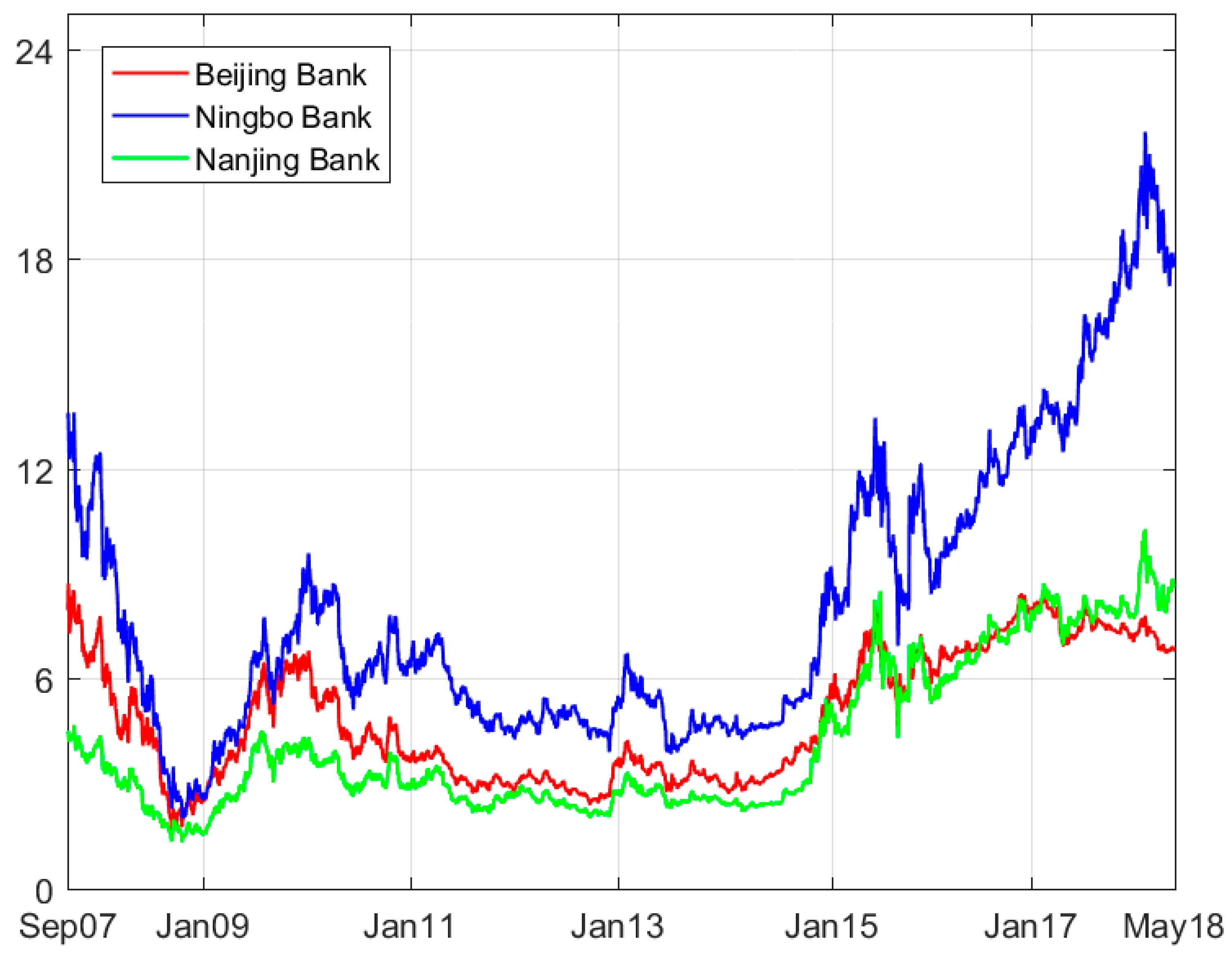
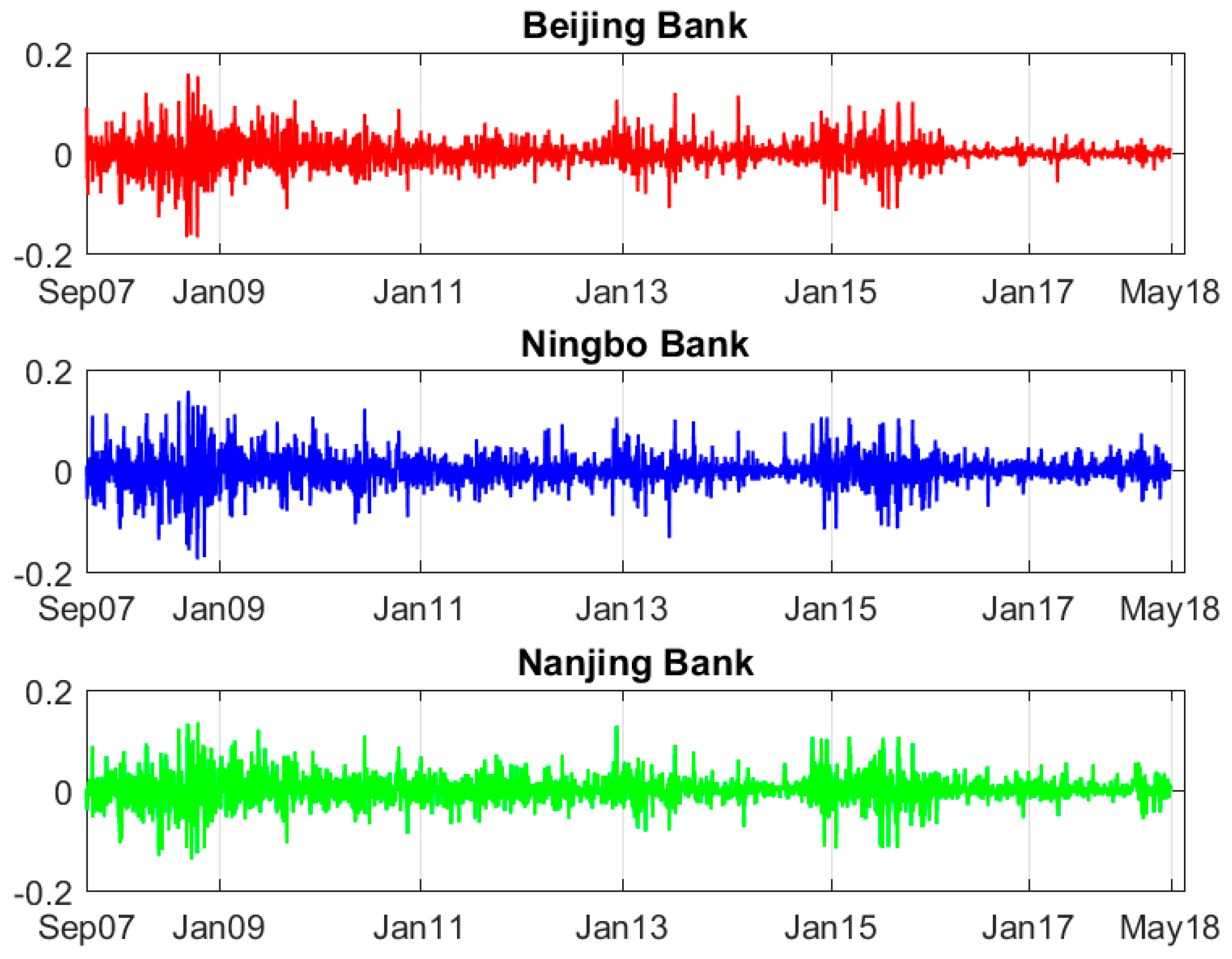
Our data contained the share price returns (based on adjusted prices) of three city banks in China: Beijing Bank, Ningbo Bank, and Nanjing Bank. The share prices and returns of these three city banks are shown in Figure 1 and Figure 2. We chose these banks not only because they are among the top five city banks in China, but also because they have stronger market liquidity in the Main Board share market, compared to that of other city banks. The share price data collected from IPOs in 2007 provided abundant data samples that covered the global financial crisis in 2008, as well as the China share market crash in late 2015. We observed large declines in share prices and high variances in returns during the global financial crisis in 2008 and the domestic stock market crash in 2015. To explore the dependence structure among these three banks, we formed three combinations: Beijing Bank and Ningbo Bank were Group 1, Beijing Bank and Nanjing Bank were Group 2, and Ningbo Bank and Nanjing Bank were Group 3.
We computed the return rates of interest using the log-difference method with the n.a. values and outliers deleted. We reported all relevant analyses in the total sample, first period sample, and second period sample. The total sample ranged from 19 September 2007 to 21 May 2018. The first period from 19 September 2007 to 4 June 2015 covered the 2008 global financial crisis. The second period from 15 June 2015 to 21 May 2018 covered the domestic stock market crash from 12 June 2015 to 19 February 2016. Descriptive statistics and the marginal distribution coefficients are given in Table 1 and Table 2, respectively.

3.2. Constant Copula Results

We used four copula models in the constant parameter case. The normal copula model, although unable to detect the tail dependence, can obtain the correlation coefficient to compare the strength of correlation in each period. The rotated Gumbel copula model, providing a higher likelihood than the normal copula, can obtain information about the lower tail dependence. Owing to this feature, we selected the rotated Gumbel copula model to capture the dependence structure changes in the joint decreases of share prices. The Student’s t copula model has the highest likelihood value and can capture tail dependence, although the lower and upper dependences are set to be equal. The SJC copula model combines the merits of the Student’s t copula and rotated Gumbel copula because it can detect potentially different dependence in both tails. In parametric distribution, the SJC copula has the least standard errors among all models.
There were several findings among the three groups based on results in Table 3, Table 4 and Table 5. First, Group 3 (Ningbo Bank and Nanjing Bank) and Group 1 (Beijing Bank and Ningbo Bank) showed the highest and lowest dependence coefficients among the three groups. This rank of dependency suggested that Beijing Bank was less dependent on the other two banks than Nanjing Bank, which was dependent on the other two banks, and that Ningbo Bank was more dependent on Nanjing Bank than on Beijing Bank. Second, Group 1 and Group 2 (Beijing Bank and Ningbo Bank) similarly showed much higher dependence in period 1 than period 2. For instance, in the rotated Student’s t copula model, the dependence coefficient ( g T ( ρ ^ , ν ^ ) ) in Groups 1 and 2 dropped 66% and 42% from period 1 to period 2, respectively. However, the dependence coefficient in Group 3 dropped only 21%. Third, the lower tail dependence was evidently higher than the upper tail dependence in the SJC copula model for Groups 1 and 2, but not for Group 3. It has been documented that the Beijing Bank share price tends to fall more frequently than rising together with the Ningbo Bank and Nanjing Bank. The probability of share prices going up was slightly higher than that of falling down together for the Ningbo Bank and Nanjing Bank group. In all groups, the Student’s t copula model had the highest value of log-likelihood, followed by the SJC copula model and the rotated Gumbel copula model.

3.3. Time-Varying Copula Results

The difference in dependence strengths between period 1 and period 2 suggested that there may be changes in tail dependence. To illustrate possible time-varying tail dependence, we constructed the rotated Gumbel copula (in GAS) and the Student’s t copula (in GAS) in a time-dependent model. The estimated parameters of the three groups are reported in Table 6, Table 7 and Table 8, respectively. The six innovation graphs of tail dependence provide visually understandable results (Figure 3, Figure 4, Figure 5, Figure 6, Figure 7 and Figure 8). The innovation in the semi-parametric models are reported.
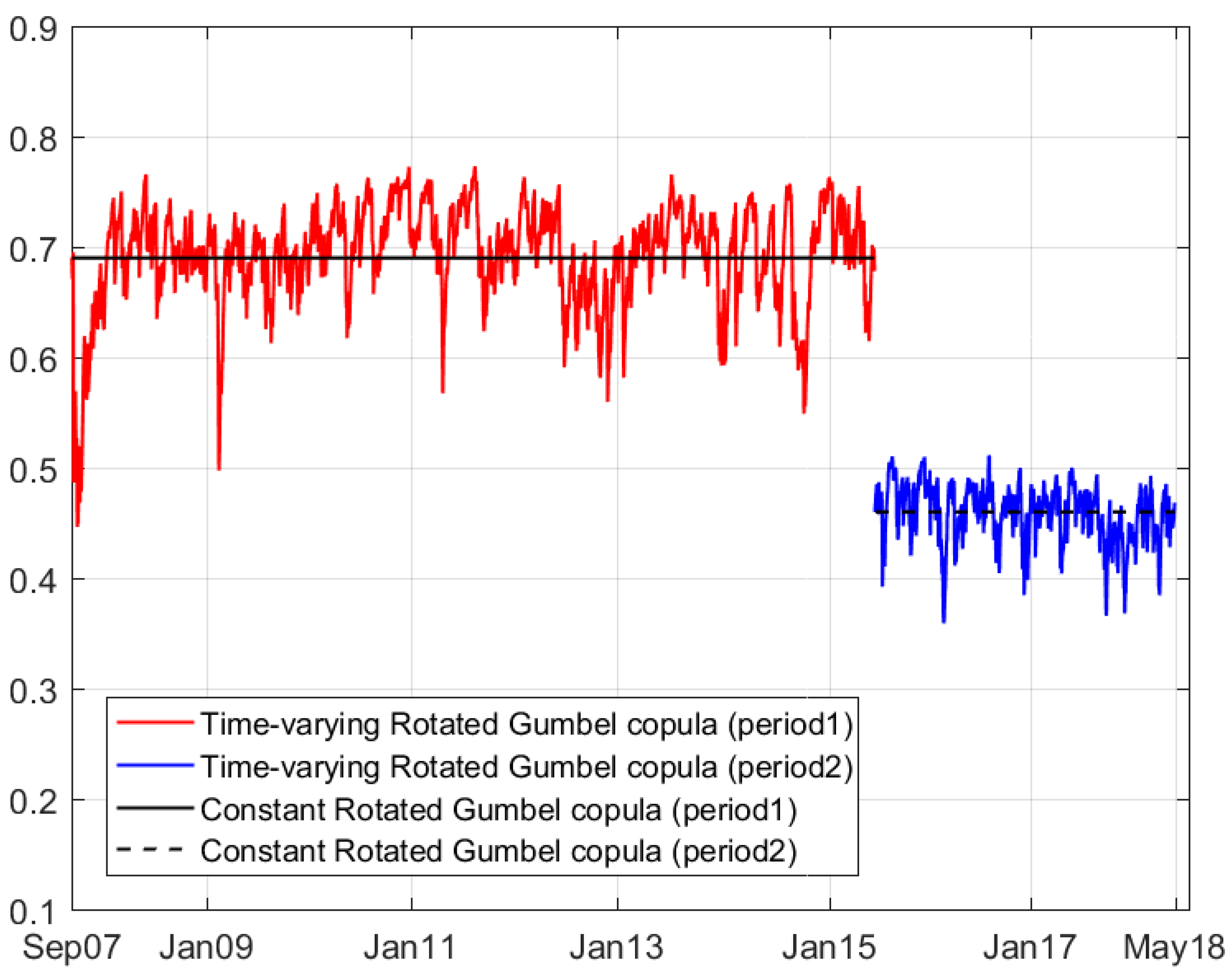
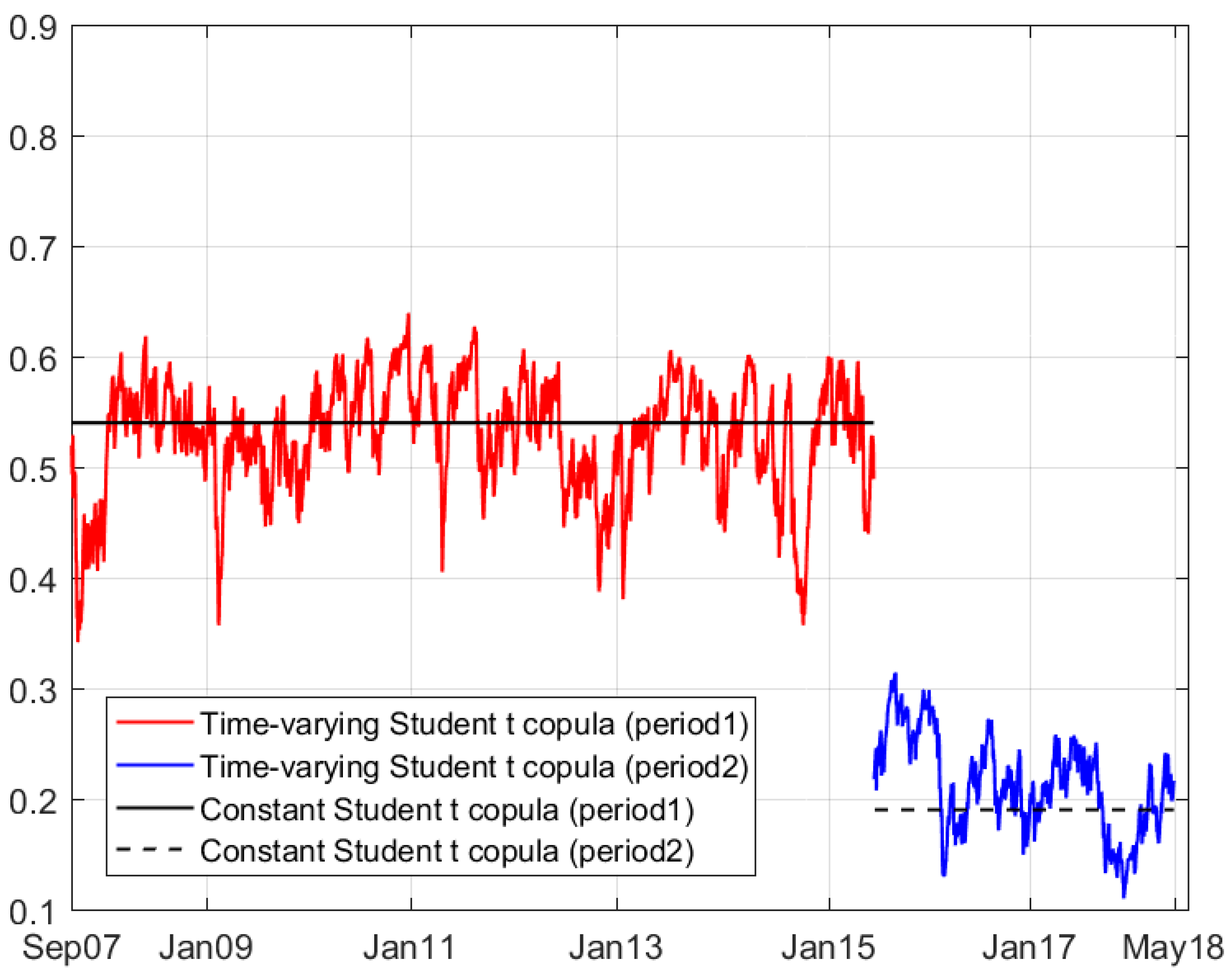
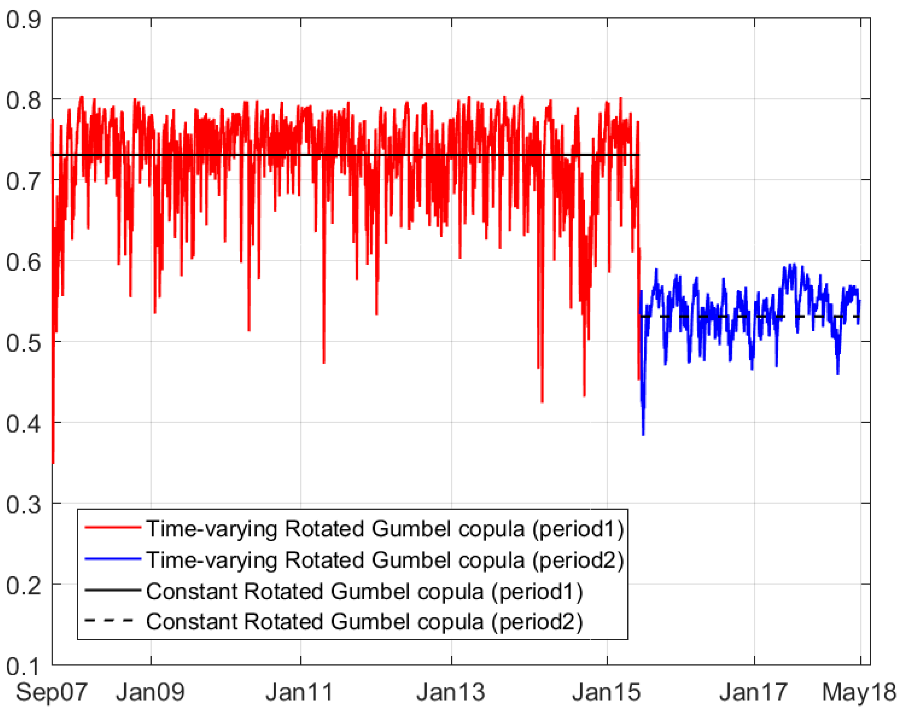
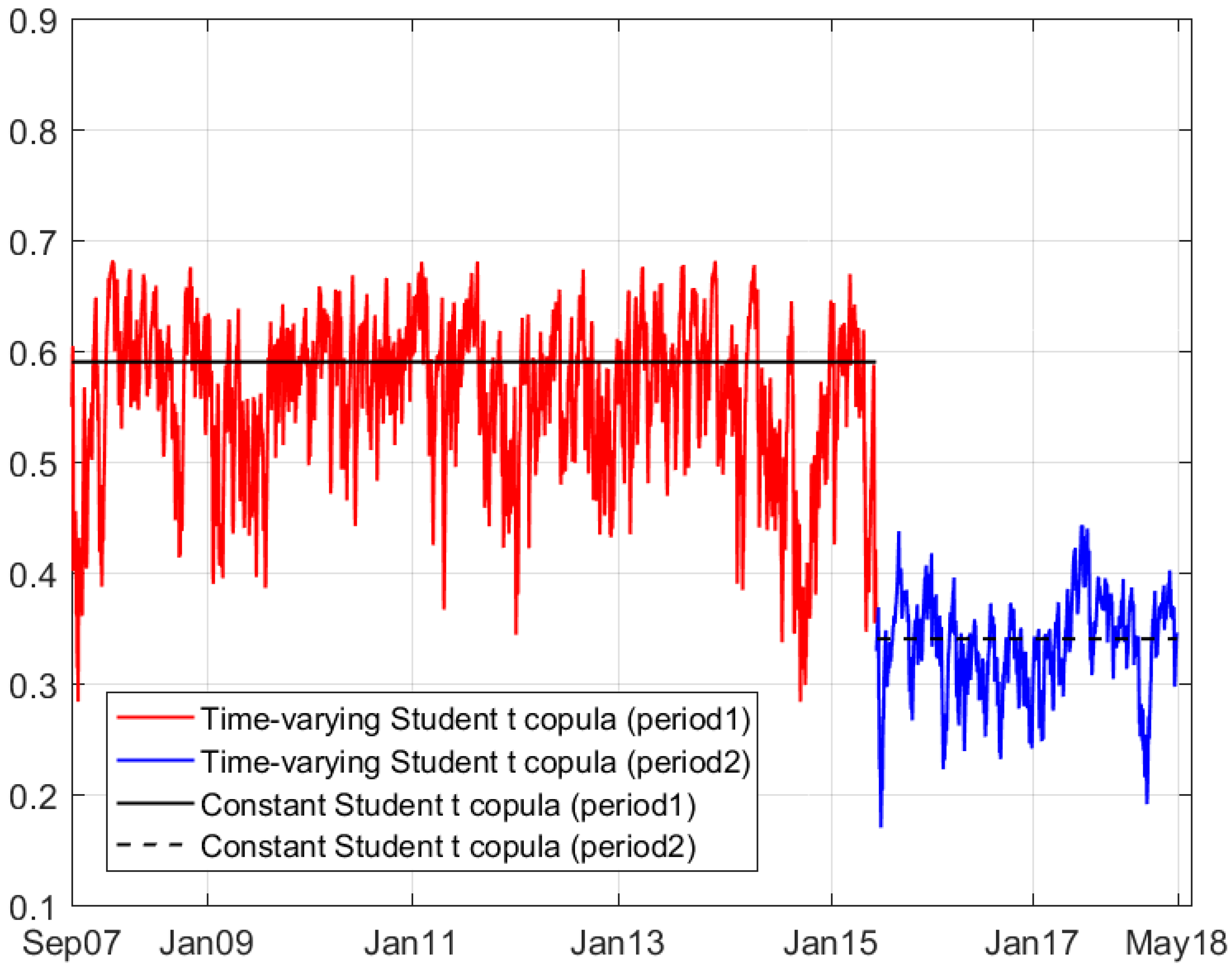
In the group of Beijing Bank and Ningbo Bank, lower tail dependence indicated by the rotated Gumbel copula (GAS) model reached the highest level of 0.75 in less than six months. Until the end of period 1, the lower tail dependence maintained a level at around 0.69, which was the tail dependence captured by the constant rotated Gumbel copula model. In period 2, the lower tail dependence fluctuated at around the level of 0.46, which was much lower than the one in period 1. In the case of the Student’s t copula (GAS) model, the innovation was similar to the one in the rotated Gumbel copula (GAS) model. The tail dependence in period 2 was less than half of the one in period 1.
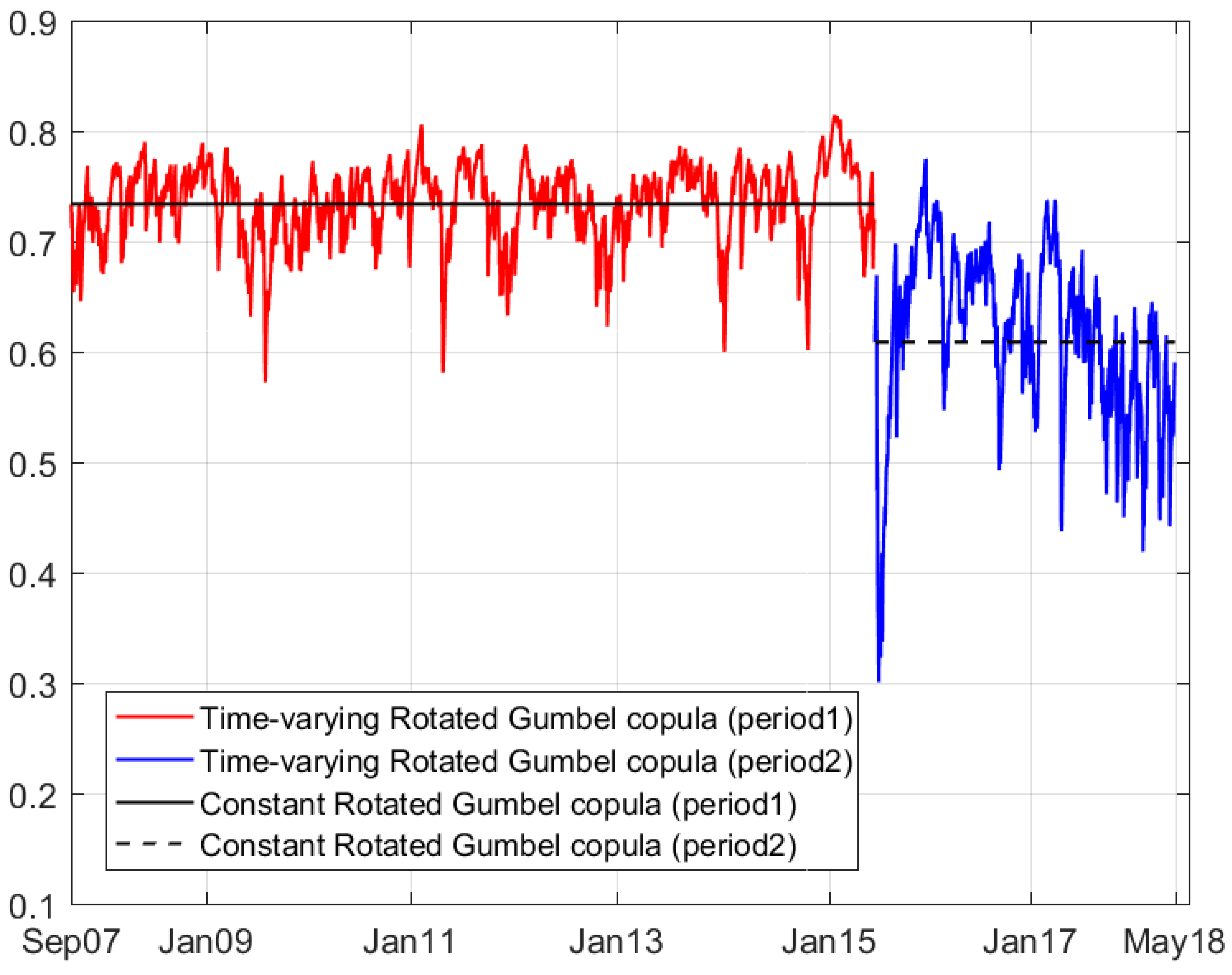
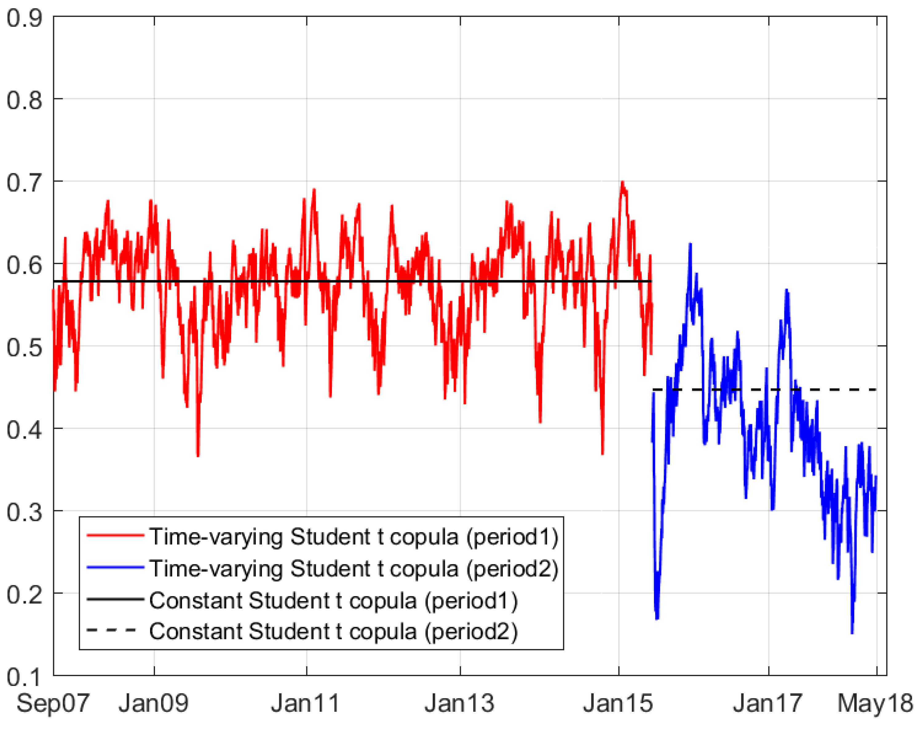
In the group consisting of Beijing Bank and Nanjing Bank, the lower tail dependence indicated by the rotated Gumbel copula (GAS) model appeared rather random after the global financial crisis, but stayed around the 0.72 level, followed by a decrease in period 2. In the Student’s t copula model, we obtained the tail dependence in period 1 in the range of around 0.59. In period 2, the dependence strength decreased to 0.34.
In the group of Ningbo Bank and Nanjing Bank, lower tail dependence indicated by the rotated Gumbel copula (GAS) model appeared rather stable after the global financial crisis and stayed around the 0.71 level, followed by a slight decrease in period 2. In the Student’s t copula model, we obtained a tail dependence in period 1 that ranged around 0.56. In period 2, the dependence strength decreased to 0.45.

3.4. Goodness-of-Fit Tests

The Kolomogorov–Smirnov (KS) and Cramer–von Mises (CvM) methods are frequently used in goodness-of-fit tests in copula models. In Table 9 and Table 10, we present the p-value results in the goodness-of-fit test for each constant copula model in the parametric and semi-parametric cases. The normal copula, rotated Gumbel copula, and the student’s t copula passed the tests in the parametric case; in the semi-parametric case, the normal copula and rotated Gumbel copula models did not pass the tests in the majority of the groups and periods, and the student’s t copula model was rejected in one test at the 5% level and in five tests at the 10% level. The SJC copula model passed the KS and CvM tests in all periods and groups, in both the parametric and semi-parametric cases. In the KS and CvM tests for time-varying copula models, the process requires the Rosenblatt transform. The two time-varying copula models passed the goodness-of-fit test in all cases (Table 11 and Table 12).

4. Conclusions

In this study on the share price returns of three city banks, we investigated the potential dependence structure. We used copula models rather than the usual linear correlation to capture the detailed tail dependence. We used various copula models to estimate the underlying dependence in extreme periods. The Student’s t, SJC, and rotated Gumbel copula models could specify the tail dependence with higher log-likelihood values better than the other copula models. Furthermore, by extending the Student’s t and rotated Gumbel copula models to the GAS and time-varying models, we could obtain more information about the innovation of changes in tail dependence.
Unlike most of the literature using copula models, we focused on the tail dependence of the share price returns of city banks rather than aggregate variables, such as share markets indices and exchange rates. The tail dependence may be dependent on profitability, own risks, inter-bank business, and outside influence. Although city banks fall in the same sector in share markets, they may have diverse returns due to different strategies or business behaviors. During and after a stock market crash, the city banks may have diverse reactions, which supports our assumption that there may be a different level of dependence between two banks during two periods.
We found diverse dependence structures among the three groups of city banks. First, the tail dependence was higher between the share price returns of Ningbo Bank and Nanjing Bank, than that of the other two combinations. Beijing Bank was less dependent on the other two city banks, and Nanjing Bank was dependent on the other two. Ningbo Bank was more dependent on Nanjing Bank, than on Beijing Bank. Second, we observed a major break in the three dependence structures. Beijing Bank became much less dependent on the other two banks during the 2015 domestic share market crash, than during the 2008 financial crisis. However, the dependency of Nanjing Bank on Ningbo Bank did not change as much as that of the other two combinations from 2008 to 2015. Third, the share prices of Ningbo Bank and Nanjing Bank had a slightly higher possibility of increasing than decreasing together. This was different from recent studies on financial asset price co-movement, which often suggest that financial assets tend to have more dependence in price crashes than in booms.
The share price returns of Ningbo Bank were found to be more similar to that of Nanjing Bank, compared to that of Beijing Bank. This observation of the share price extreme returns of three city banks reconfirmed our research results in the copula models. Risk-avoiding behavior is a possible cause of the decrease in tail dependence. It is recommended that for city commercial banks, strategies such as obtaining superior assets and involving less risky inter-bank business be adopted, and that for the central bank, reasonable capital liquidity and supervision should be ensured to create a healthier inter-bank market. Nowadays, the majority of local Chinese companies are experiencing low profit margins. The central and local governments should help boost the domestic economy, under both fiscal and monetary policies, and avoid the crisis from happening in the real economy, which may transmit to banking systems.

Author Contributions

S.H. conceived and designed the experiments; G.L. performed the experiments, analyzed the data, and contributed reagents/materials/analysis tools; G.L., X.-J.C., and S.H. wrote the paper.

Funding

This research was funded by JSPS KAKENHI Grant Number 17K18564 and (A) 17H00983.

Acknowledgments

We are grateful to three anonymous referees for their helpful comments and suggestions. We are also grateful to the participants of The SIBR 2018 Hong Kong Conference on Interdisciplinary Business & Economics Research for helpful comments.

Conflicts of Interest

The authors declare no conflict of interest. The founding sponsors had no role in the design of the study, in the collection, analyses, or interpretation of data, in the writing of the manuscript, or in the decision to publish the results.

References

  1. Ang, Andrew, and Joseph Chen. 2002. Asymmetric correlations of equity portfolios. Journal of Financial Economics 63: 443–94. [Google Scholar] [CrossRef]
  2. Bollerslev, Tim. 1987. A conditionally heteroskedastic time series model for speculative prices and rates of return. The Review of Economics and Statistics 69: 542–47. [Google Scholar] [CrossRef]
  3. Casella, G., and Roger L. Berger. 1990. Statistical Inference. Belmont: Duxbury Press. [Google Scholar]
  4. Creal, D., Siem Jan Koopman, and André Lucas. 2013. Generalized autoregressive score models with applications. Journal of Applied Econometrics 28: 777–95. [Google Scholar] [CrossRef]
  5. Fama, Eugene F. 1965. The behavior of stock-market prices. The Journal of Business 38: 34–105. [Google Scholar] [CrossRef]
  6. Gumbel, Emil J. 1960. Bivariate exponential distributions. Journal of the American Statistical Association 55: 698–707. [Google Scholar] [CrossRef]
  7. Hansen, Bruce E. 1994. Autoregressive conditional density estimation. International Economic Review, 705–30. [Google Scholar] [CrossRef]
  8. Joe, Harry. 1997. Multivariate Models and Multivariate Dependence Concepts. Boca Raton: CRC Press. [Google Scholar]
  9. Luo, W., Robert D. Brooks, and Param Silvapulle. 2011. Effects of the open policy on the dependence between the Chinese ‘A’ stock market and other equity markets: An industry sector perspective. Journal of International Financial Markets, Institutions and Money 21: 49–74. [Google Scholar] [CrossRef]
  10. Marimoutou, Vêlayoudom, and Manel Soury. 2015. Energy markets and CO2 emissions: Analysis by stochastic copula autoregressive model. Energy 88: 417–29. [Google Scholar] [CrossRef]
  11. Patton, Andrew J. 2006. Modelling asymmetric exchange rate dependence. International Economic Review 47: 527–56. [Google Scholar] [CrossRef]
  12. Patton, Andrew J. 2013. Copula methods for forecasting multivariate time series. In Handbook of Economic Forecasting. New York: Elsevier, vol. 2, pp. 899–960. [Google Scholar] [CrossRef]
  13. Reboredo, Juan C., and Andrea Ugolini. 2015. Downside/upside price spillovers between precious metals: A vine copula approach. The North American Journal of Economics and Finance 34: 84–102. [Google Scholar] [CrossRef]
  14. Sklar, Abe. 1959. Fonctions de répartition à n dimensions et leurs marges. Publications de l’Institut de Statistique de l’Université de Paris 8: 229–31. [Google Scholar]
  15. Sukcharoen, Kunlapath, Tatevik Zohrabyan, David Leatham, and Ximing Wu. 2014. Interdependence of oil prices and stock market indices: A copula approach. Energy Economics 44: 331–39. [Google Scholar] [CrossRef]
Figure 1. Daily share prices of the Beijing Bank, Ningbo Bank, and Nanjing Bank from 19 September 2007 to 21 May 2018.
Jrfm 11 00057 g001
Figure 2. Daily returns of the Beijing Bank, Ningbo Bank, and Nanjing Bank from 19 September 2007 to 21 May 2018.
Jrfm 11 00057 g002
Figure 3. Time-varying and constant tail dependence in the Rotated Gumbel copula for Group 1 (Beijing Bank and Ningbo Bank). Period 1 ranges from 19 September 2007 to 4 June 2015 and period 2 ranges from 15 June 2015 to 21 May 2018.
Jrfm 11 00057 g003
Figure 4. Time-varying and constant tail dependence in the Student’s t copula for Group 1 (Beijing Bank and Ningbo Bank). Period 1 ranges from 19 September 2007 to 4 June 2015 and period 2 ranges from 15 June 2015 to 21 May 2018.
Jrfm 11 00057 g004
Figure 5. Time-varying and constant tail dependence in the Rotated Gumbel copula for Group 2 (Beijing Bank and Nanjing Bank). Period 1 ranges from 19 September 2007 to 4 June 2015 and period 2 ranges from 15 June 2015 to 21 May 2018.
Jrfm 11 00057 g005
Figure 6. Time-varying and constant tail dependence in the Student’s t copula for Group 2 (Beijing Bank and Nanjing Bank). Period 1 ranges from 19 September 2007 to 4 June 2015 and period 2 ranges from 15 June 2015 to 21 May 2018.
Jrfm 11 00057 g006
Figure 7. Time-varying and constant tail dependence in the Rotated Gumbel copula for Group 3 (Ningbo Bank and Nanjing Bank). Period 1 ranges from 19 September 2007 to 4 June 2015 and period 2 ranges from 15 June 2015 to 21 May 2018.
Jrfm 11 00057 g007
Figure 8. Time-varying and constant tail dependence in the Student’s t copula for Group 3 (Ningbo Bank and Nanjing Bank). Period 1 ranges from 19 September 2007 to 4 June 2015 and period 2 ranges from 15 June 2015 to 21 May 2018.
Jrfm 11 00057 g008
Table 1. Descriptive statistics of share price returns.
MeanS.E.MinMaxSkewnessKurtosisJarque−Bera
Beijing Bank
Total0.00010.0273−0.16790.1584−0.034711.46683075.041
Period 10.00030.0301−0.16790.1584−0.038010.19961320.999
Period 2−0.00040.0180−0.11190.1022−0.127418.12984121.534
Ningbo Bank
Total0.00020.0309−0.17730.1586−0.074310.26971877.701
Period 10.00030.0331−0.17730.1586−0.02749.79591079.081
Period 2−0.00010.0242−0.11440.1037−0.413710.6811632.7394
Nanjing Bank
Total0.00040.0274−0.13870.13350.034010.07551709.185
Period 10.00060.0289−0.13870.13350.19039.3543853.2647
Period 2−0.00020.0231−0.11580.1054−0.831913.04021465.303
Notes: Period 1 ranges from 19 September 2007 to 4 June 2015 and period 2 ranges from 15 June 2015 to 21 May 2018. Observations of the total sample, first period, and second period were 2469, 1797, and 672, respectively. The table displays the basic summary statistics of the total sample, first period sample, and second period sample. As usual, financial asset returns show skewness around zero and kurtosis larger than three, indicating a non-normal distribution. The Jarque–Bera test statistics are reported, all of which stayed significant at 1%, indicating a non-normal distribution.
Table 2. Marginal distribution parameters estimation result.
TotalPeriod 1Period 2
Beijing Bank
Mean Model
φ 0 6 × 10 5 (0.0003)−0.0001(0.0005)−0.0002(0.0003)
  φ 1 −0.0584 ***(0.0192)−0.0667 ***(0.0227)−1.5568 ***(0.0168)
  φ 2 ------------−1.2535 ***(0.0154)
  φ 3 −0.6816 ***(0.0239)
  φ 4 −0.0164(0.0206)
  θ 1 1.5119 ***(0.0001)
  θ 2 1.0736 ***(0.0002)
  θ 3 0.5416 ***(0.0007)
Variance model
  ω 0.0000---0.0000---0.0000---
  α 0.0669 ***(0.0200)0.0607 ***(0.0139)0.1553 ***(0.0451)
  Β 0.9321 ***(0.0196)0.9376 ***(0.0139)0.8435 ***(0.0368)
  ν 4.6502 ***(0.4315)4.7860 ***(0.5694)3.1771 ***(0.3759)
Skewed t density
  λ 0.02720.0208−0.0005
  ν 4.54134.53363.2202
Ljung–Box test
  Q ( 20 ) 6.8882(0.9970)4.7600(0.9998)28.4805(0.0985)
  Q 2 ( 20 ) 23.6720(0.2570)16.5393(0.6827)19.6328(0.4811)
GoF tests on skewed t distribution model (p value)
KS0.960.990.99
CvM0.950.990.99
Ningbo Bank
Mean model
  φ 0 0.0003(0.0004)0.0003(0.0005)0.0005(0.0005)
  φ 1 ------------1.4112 ***(0.0300)
  φ 2 −1.6308 ***(0.0293)
  φ 3 1.3830 ***(0.0307)
  φ 4 −0.6112 ***(0.0165)
  θ 1 −1.4267 ***(0.0120)
  θ 2 1.5598 ***(0.0326)
  θ 3 −1.3749 ***(0.0162)
  θ 4 0.5695 ***(0.0044)
Variance model
  ω 0.0000---0.0000---0.0000---
  α 0.0564 ***(0.0187)0.0462 ***(0.0074)0.1148 ***(0.0397)
  Β 0.9426 ***(0.0191)0.9528 ***(0.0071)0.8366 ***(0.0508)
  ν 4.3642 ***(0.4138)4.4861 ***(0.5291)4.1153 ***(0.6908)
Skewed t density
  λ 0.02410.00610.0161
  ν 4.23824.31574.3207
Ljung–Box test
  Q ( 20 ) 22.2234(0.3285)13.2727(0.8654)20.1693(0.4474)
  Q 2 ( 20 ) 24.9517(0.2033)19.9116(0.4635)22.6349(0.3071)
GoF tests on skewed t distribution model (p value)
KS0.890.880.44
CvM0.970.940.22
Nanjing Bank
Mean model
  φ 0 0.0002(0.0004)0.0001(0.0004)0.0001(0.0001)
  φ 1 ------0.3352(0.3948)−0.0700 *** ( 3 × 10 5 )
  φ 2 ------−0.0381 *** ( 1 × 10 5 )
  φ 3 −0.0996 *** ( 3 × 10 5 )
  φ 4 0.9056 ***(0.0002)
  θ 1 −0.4203(0.3801)0.0627 *** ( 3 × 10 5 )
  θ 2 ------−0.0162 *** ( 3 × 10 5 )
  θ 3 0.0386 *** ( 2 × 10 5 )
  θ 4 −0.9260 ***(0.0002)
Variance model
  ω 0.0000---0.0000---0.0000---
  α 0.0682 ***(0.024)0.0504 **(0.0205)0.1769 ***(0.0627)
  β 0.9308 ***(0.0257)0.9486 ***(0.0226)0.8068 ***(0.0517)
  ν 4.2478 ***(0.3742)4.2761 ***(0.4511)3.3927 ***(0.5039)
Skewed t density
  λ 0.03270.03460.0077
  ν 4.17474.18713.4216
Ljung–Box test
  Q ( 20 ) 8.7088(0.9860)11.3141(0.9377)26.2620(0.1573)
  Q 2 ( 20 ) 22.0430(0.3382)18.9296(0.5264)20.0537(0.4546)
GoF tests on skewed t distribution model (p value)
KS0.660.790.37
CvM0.870.840.31
Notes: The table summarizes the coefficients of the ARMA model for each bank’s share returns, and standard GARCH (1,1) for all three share price return residuals. Period 1 ranges from 19 September 2007 to 4 June 2015 and period 2 ranges from 15 June 2015 to 21 May 2018. For each parameter, standard errors are reported in parentheses with *** and ** representing the significance levels of 1% and 5%, respectively. In all GARCH models, ω was estimated to be zero and thus standard residuals are not reported. We estimated the skewness parameter λ and a degrees of freedom parameter ν in the skewed t model. Q ( 20 ) statistics and p-values were given under the null hypothesis of the Ljung–Box test, so that no autocorrelation existed in standardized residuals up to lags 20, with Q 2 ( 20 ) representing the test on squared standardized residuals up to lags 20. All results from the Ljung–Box test showed that the squared standardized residuals in each estimation model of the three bank shares in the total sample and two distinct samples had no significant evidence of autocorrelation up to lags 20. All insignificant p-values in the KS and CvM test (goodness of fit test, GOF) indicated that we failed to reject the null hypothesis, which states that the skewed t model can well specify the distribution of standardized residuals in all share price returns.
Table 3. Constant copula models in Group 1, consisting of the Beijing Bank and Ningbo Bank.
TotalPeriod 1Period 2
ParametricSemiParametricSemiParametricSemi
Normal copula
ρ ^ 0.76690.76620.82370.82280.58170.5795
S.E.(0.0135)(0.0104)(0.011)(0.0108)(0.0369)(0.0266)
log L 1094.031091.711019.281015.47139.17137.49
Rotated Gumbel copula
γ ^ 2.19762.23102.54922.56861.60661.6043
S.E.(0.0819)(0.0393)(0.0875)(0.0582)(0.0891)(0.0530)
τ ^ L 0.62920.63560.68750.69020.46050.4596
log L 1107.791111.691031.201029.37135.62134.72
Student’s t copula
ρ ^ 0.76840.77310.82680.82810.57590.5800
S.E.(0.0145)(0.008)(0.011)(0.0085)(0.0368)(0.0255)
ν ^ 1 0.27930.29700.28070.28970.14580.1496
S.E.(0.0286)(0.028)(0.0401)(0.0331)(0.0560)(0.0405)
g T ( ρ ^ , ν ^ ) 0.47660.49300.54240.54950.18470.1923
log L 1192.441192.731100.101097.01144.47142.93
SJC copula
τ ^ L 0.59640.60900.66970.67480.39980.4039
S.E. ( 9 × 10 16 )(0.0143) ( 1 × 10 15 )(0.0136) ( 5 × 10 17 )(0.0373)
τ ^ U 0.58150.59370.65670.66330.36230.3736
S.E. ( 9 × 10 16 )(0.0167) ( 1 × 10 15 )(0.0173) ( 1 × 10 16 )(0.0451)
log L 1156.341161.09391073.601074.64145.01143.32
Notes: In this table, we report the maximum likelihood estimation and standard errors in parentheses. “Parametric” and “Semi” represent the parametric and semi-parametric models, respectively. Period 1 ranges from 19 September 2007 to 4 June 2015 and period 2 ranges from 15 June 2015 to 21 May 2018. Lower tail dependence of the rotated Gumbel copula was calculated by τ ^ L = 2 2 1 / γ ^ . Both tail dependences in the Student’s t copula were calculated in g T ( ρ ^ , ν ^ ) = 2 × F s t u d e n t ( ( ν ^ + 1 ) ρ ^ 1 ρ ^ + 1 , ν ^ + 1 ) .
Table 4. Constant copula models in Group 2, consisting of the Beijing Bank and Nanjing Bank.
TotalPeriod 1Period 2
ParametricSemiParametricSemiParametricSemi
Normal copula
ρ ^ 0.81190.81150.85640.85560.64870.6422
S.E.(0.0128)(0.0083)(0.0105)(0.0084)(0.0271)(0.0311)
log L 1328.561326.631187.931183.38183.89178.64
Rotated Gumbel copula
γ ^ 2.44862.49672.85282.87991.82401.8076
S.E.(0.0926)(0.0482)(0.1002)(0.0638)(0.0822)(0.0673)
τ ^ L 0.67280.68000.72500.72790.53770.5326
log L 1347.261351.381209.541207.97196.85190.97
Student’s t copula
ρ ^ 0.81260.81760.86010.86130.65510.6563
S.E.(0.0129)(0.0066)(0.0099)(0.0065)(0.0264)(0.0264)
ν ^ 1 0.26160.28380.28410.29450.23700.2393
S.E.(0.0329)(0.0267)(0.0334)(0.0325)(0.0592)(0.0500)
g T ( ρ ^ , ν ^ ) 0.51270.53340.58770.59510.34290.3459
log L 1424.531427.291269.651266.36207.44202.25
SJC copula
τ ^ L 0.65590.66870.72040.72660.51840.5109
S.E. ( 1 × 10 15 )(0.0147) ( 8 × 10 16 )(0.0129) ( 5 × 10 16 )(0.0305)
τ ^ U 0.61470.63220.67860.68460.41140.4228
S.E. ( 4 × 10 16 )(0.0154) ( 8 × 10 16 )(0.027) ( 4 × 10 16 )(0.0488)
log L 1378.741389.561229.001230.85201.73195.47
Notes: In this table, we report the maximum likelihood estimation and standard errors in parentheses. “Parametric” and “Semi” represent the parametric and semi-parametric models, respectively. Period 1 ranges from 19 September 2007 to 4 June 2015 and period 2 ranges from 15 June 2015 to 21 May 2018. Lower tail dependence of the rotated Gumbel copula was calculated as τ ^ L = 2 2 1 / γ ^ . Both tail dependences in the Student’s t copula were calculated in g T ( ρ ^ , ν ^ ) = 2 × F s t u d e n t ( ( ν ^ + 1 ) ρ ^ 1 ρ ^ + 1 , ν ^ + 1 ) .
Table 5. Constant copula models in Group 3, consisting of the Ningbo Bank and Nanjing Bank.
TotalPeriod 1Period 2
ParametricSemiParametricSemiParametricSemi
Normal copula
ρ ^ 0.84610.84510.87140.87050.73760.7347
S.E.(0.0090)(0.0072)(0.0081)(0.0068)(0.0253)(0.0214)
log L 1552.991546.231279.921274.06264.24260.76
Rotated Gumbel copula
γ ^ 2.70772.71672.90712.93722.11902.0990
S.E.(0.0876)(0.0530)(0.1260)(0.0605)(0.1431)(0.0872)
τ ^ L 0.70830.70940.73070.73380.61300.6087
log L 1539.471534.071251.241247.42269.94264.34
Student’s t copula
ρ ^ 0.84830.84920.87010.87190.74800.7479
S.E.(0.0091)(0.0059)(0.0128)(0.0055)(0.0251)(0.0182)
ν ^ 1 0.26200.27020.22830.24070.27690.2648
S.E.(0.0310)(0.0280)(0.0404)(0.0333)(0.0594)(0.0441)
g T ( ρ ^ , ν ^ ) 0.55820.56460.56590.57760.45490.4460
log L 1650.471643.971332.231328.24292.83285.36
SJC copula
τ ^ L 0.68060.68390.71020.71600.56110.5570
S.E. ( 1 × 10 14 )(0.0130) ( 1 × 10 16 )(0.0123) ( 1 × 10 15 )(0.0390)
  τ ^ U 0.69120.69930.71830.72810.57390.5769
S.E. ( 9 × 10 15 )(0.0120) ( 5 × 10 16 )(0.0108) ( 9 × 10 16 )(0.0287)
  log L 1604.251605.731304.741309.07282.73275.45
Notes: In this table, we report the maximum likelihood estimation and standard errors in parentheses. “Parametric” and “Semi” represent the parametric and semi-parametric models, respectively. Period 1 ranges from 19 September 2007 to 4 June 2015 and period 2 ranges from 15 June 2015 to 21 May 2018. Lower tail dependence of the rotated Gumbel copula was calculated in τ ^ L = 2 2 1 / γ ^ . Both tail dependences in the Student’s t copula were calculated in g T ( ρ ^ , ν ^ ) = 2 × F s t u d e n t ( ( ν ^ + 1 ) ρ ^ 1 ρ ^ + 1 , ν ^ + 1 ) .
Table 6. Time-varying copula models in Group 1 (Beijing Bank and Ningbo Bank).
TotalPeriod 1Period 2
ParametricSemiParametricSemiParametricSemi
Rotated Gumbel copula (GAS)
  ω ^ 0.00190.00210.02590.0302–0.0837–0.0833
S.E.(0.0155)(0.0001)(0.0072)(0.0043)(0.0004)(0.0543)
  α ^ 0.06500.05930.08320.09050.06300.0675
S.E.(0.0622)(0.0018)(0.0199)(0.0176)(0.0012)(0.0569)
  β ^ 0.98920.99060.94470.93690.83550.8397
S.E.(0.0014)(0.0005)(0.0143)(0.0061)(0.0327)(0.1143)
  log L 1185.621187.581053.581050.44136.41135.64
Student’s t copula (GAS)
  ω ^ 0.02180.02130.10120.10040.01920.0300
S.E.(0.0018)(0.0018) ( 2 × 10 9 )(0.0036)(0.0296)(0.0038)
  α ^ 0.06340.06320.07400.07240.02610.0516
S.E.(0.0052)(0.0102) ( 4 × 10 8 )(0.0109)(0.0139)(0.0202)
  β ^ 0.98970.98960.95840.95850.98430.9764
S.E. ( 5 × 10 6 ) ( 6 × 10 7 ) ( 4 × 10 7 ) ( 1 × 10 7 )(0.0228)(0.0123)
  ν ^ 1 0.21740.21850.24130.24470.15900.1687
S.E.(0.0219)(0.0285)(0.0314)(0.0338)(0.0479)(0.0442)
  log L 1273.171271.041117.501114.18146.96145.95
Notes: In this table, we report the maximum likelihood estimation and standard errors in parentheses. “Parametric” and “Semi” represent the parametric and semi-parametric models, respectively. Period 1 ranges from 19 September 2007 to 4 June 2015 and period 2 ranges from 15 June 2015 to 21 May 2018.
Table 7. Time-varying copula models in Group 2 (Beijing Bank and Nanjing Bank).
TotalPeriod 1Period 2
ParametricSemiParametricSemiParametricSemi
Rotated Gumbel copula (GAS)
  ω ^ 0.01800.01770.13130.1390−0.0282−0.0230
S.E.(0.0022)(0.0026)(0.0018)(0.6113)(0.0478)(0.1966)
  α ^ 0.12710.12340.22250.21590.11310.1018
S.E.(0.0169)(0.0220)(0.0214)(0.2863)(0.1006)(0.0790)
  β ^ 0.95560.95560.78550.78160.78770.8301
S.E. ( 2 × 10 5 ) ( 2 × 10 5 )(0.0036)(0.8849)(0.2617)(0.8756)
  log L 1426.911425.741247.191243.53219.16214.94
Student’s t copula (GAS)
  ω ^ 0.10150.10010.50770.29210.13390.1192
S.E.(0.0584)(0.0043) ( 4 × 10 8 )(0.0089)(0.1118)(0.0084)
  α ^ 0.13640.13160.21030.16200.11050.0849
S.E.(0.0627)(0.0190)(0.0298)(0.0290)(0.0374)(0.0203)
  β ^ 0.95680.95800.80800.88980.92010.9287
S.E.(0.0258) ( 5 × 10 6 ) ( 7 × 10 6 ) ( 4 × 10 6 )(0.0649) ( 8 × 10 6 )
  ν ^ 1 0.19860.21750.22660.22460.20600.2034
S.E.(0.0367)(0.0212)(0.0334)(0.0336)(0.0396)(0.0444)
  log L 1513.261513.641309.931306.48229.49224.16
Notes: In this table, we report the maximum likelihood estimation and standard errors in parentheses. “Parametric” and “Semi” represent the parametric and semi-parametric models, respectively. Period 1 ranges from 19 September 2007 to 4 June 2015 and period 2 ranges from 15 June 2015 to 21 May 2018.
Table 8. Time-varying copula models in Group 3 (Ningbo Bank and Nanjing Bank).
TotalPeriod 1Period 2
ParametricSemiParametricSemiParametricSemi
Rotated Gumbel copula (GAS)
  ω ^ 0.01630.01570.03980.04780.01020.0074
S.E.(0.0007)(0.0021)(0.0005)(0.0017)(0.0043)(0.0024)
  α ^ 0.08480.08040.08570.08550.12160.1228
S.E.(0.0138)(0.0278)(0.0210)(0.0257)(0.0747)(0.0269)
  β ^ 0.97120.97270.93880.92910.95260.9461
S.E.(0.0014)(0.0012)(0.0008)(0.0014)(0.0560)(0.0030)
  log L 1595.391586.461270.491264.77287.67280.34
Student’s t copula (GAS)
  ω ^ 0.07480.07460.13830.14460.03640.0477
S.E.(0.0031)(0.0034)(0.0050)(0.0003)(0.0142)(0.0057)
  α ^ 0.09910.09930.09230.09290.10470.1016
S.E.(0.0205)(0.0253)(0.0430)(0.0223)(0.0205)(0.0344)
  β ^ 0.97060.97070.94900.94720.98150.9762
S.E. ( 4 × 10 6 ) ( 1 × 10 5 ) ( 3 × 10 5 ) (0.0017)(0.0073) ( 8 × 10 7 )
  ν ^ 1 0.22520.22520.22550.22780.24600.1939
S.E.(0.0239)(0.0392)(0.0391)(0.0343)(0.0382)(0.0437)
  log L 1713.661704.271356.181350.24309.03301.51
Notes: In this table, we report the maximum likelihood estimation and standard errors in parentheses. “Parametric” and “Semi” represent the parametric and semi-parametric models, respectively. Period 1 ranges from 19 September 2007 to 4 June 2015 and period 2 ranges from 15 June 2015 to 21 May 2018.
Table 9. Goodness-of-fit test in the constant copula (parametric case).
TotalPeriod 1Period 2
K S C   C v M C   K S C   C v M C   K S C   C v M C  
Normal copula
Group 10.920.970.960.980.990.94
Group 20.800.950.930.960.990.98
Group 30.820.960.930.940.380.33
Rotated Gumbel copula
Group 10.950.930.970.950.980.94
Group 20.910.950.950.910.990.97
Group 30.870.920.920.930.260.21
Student’s t copula
Group 10.960.980.970.990.990.97
Group 20.800.960.920.960.990.98
Group30.880.970.940.960.340.30
SJC copula
Group10.940.950.950.960.990.99
Group20.810.910.800.880.990.99
Group30.860.950.890.890.490.43
Notes: In this table, we report the p-values of the Kolomogorov–Smirnov ( K S C ) and Cramer–von Mises ( C v M C ) goodness-of-fit tests for the constant copula models in the parametric case, based on 500 simulations. The subscript C indicates that the test was carried out on the empirical copula of the standardized residuals. Group 1 refers to the group of Beijing Bank and Ningbo Bank. Group 2 refers to the group of Beijing Bank and Nanjing Bank. Group 3 refers to the group of Ningbo Bank and Nanjing Bank. Period 1 ranges from 19 September 2007 to 4 June 2015 and period 2 ranges from 15 June 2015 to 21 May 2018. p-values less than 0.05 are shown in bold.
Table 10. Goodness-of-fit test in constant copula (semi-parametric case).
TotalPeriod 1Period 2
  K S C     C v M C     K S C     C v M C     K S C     C v M C  
Normal copula
Group10.170.010.140.000.910.61
Group20.090.010.020.000.220.24
Group30.070.010.090.040.150.02
Rotated Gumbel copula
Group10.000.000.000.000.120.00
Group20.000.000.000.000.130.00
Group30.000.000.000.000.000.00
Student’s t copula
Group10.620.540.040.100.880.70
Group20.480.500.050.070.580.63
Group30.170.290.440.230.500.10
SJC copula
Group10.990.990.990.990.990.99
Group20.990.990.990.990.990.99
Group30.990.990.990.990.990.99
Notes: In this table, we report the p-values of the Kolomogorov–Smirnov ( K S C ) and Cramer–von Mises ( C v M C ) goodness-of-fit tests for the constant copula models in the semi-parametric case, based on 500 simulations. The subscript C indicates that the test was carried out on the empirical copula of the standardized residuals. Group 1 refers to the group of Beijing Bank and Ningbo Bank. Group 2 refers to the group of Beijing Bank and Nanjing Bank. Group 3 refers to the group of Ningbo Bank and Nanjing Bank. Period 1 ranges from 19 September 2007 to 4 June 2015 and period 2 ranges from 15 June 2015 to 21 May 2018. p-values less than 0.05 are shown in bold.
Table 11. Goodness-of-fit test in time-varying copula (parametric case).
TotalPeriod 1Period 2
K S R   C v M R   K S R   C v M R   K S R   C v M R  
Rotated Gumbel copula (GAS)
Group 10.990.990.990.990.970.96
Group 20.990.990.990.880.990.99
Group 30.990.990.970.970.800.69
Student’s t copula (GAS)
Group 10.990.990.990.990.990.99
Group 20.990.990.980.990.990.99
Group 30.990.990.960.970.920.81
Notes: In this table, we report the p-values of the Kolomogorov–Smirnov ( K S R ) and Cramer–von Mises ( C v M R ) goodness-of-fit tests for the time-varying copula models in the parametric case, based on 100 simulations. The subscript R indicates that the test was carried out on the empirical copula of the Rosenblatt transform of the residuals. Group 1 refers to the group of Beijing Bank and Ningbo Bank. Group 2 refers to the group of Beijing Bank and Nanjing Bank. Group 3 refers to the group of Ningbo Bank and Nanjing Bank. Period 1 ranges from 19 September 2007 to 4 June 2015 and period 2 ranges from 15 June 2015 to 21 May 2018.
Table 12. Goodness-of-fit test in time-varying copula (semi-parametric case).
TotalPeriod 1Period 2
K S R   C v M R   K S R   C v M R   K S R   C v M R  
Rotated Gumbel copula (GAS)
Group 10.810.990.240.970.090.33
Group 20.830.990.980.990.470.44
Group 30.850.990.930.990.930.88
Student’s t copula (GAS)
Group 10.630.590.390.400.660.57
Group 20.990.890.660.670.960.96
Group 30.580.800.500.600.610.62
Notes: In this table, we report the p-values of the Kolomogorov–Smirnov ( K S R ) and Cramer–von Mises ( C v M R ) goodness-of-fit tests for the time-varying copula models in the semi-parametric case, based on 100 simulations. The subscript R indicates that the test was carried out on the empirical copula of the Rosenblatt transform of the residuals. Group 1 refers to the group of Beijing Bank and Ningbo Bank. Group 2 refers to the group of Beijing Bank and Nanjing Bank. Group 3 refers to the group of Ningbo Bank and Nanjing Bank. Period 1 ranges from 19 September 2007 to 4 June 2015 and period 2 ranges from 15 June 2015 to 21 May 2018.

