On the Performance of Wavelet Based Unit Root Tests

1
Department of Economics, Istanbul Bilgi University, Istanbul 34060, Turkey
2
Institute of Graduate Programs, Istanbul Bilgi University, Istanbul 34060, Turkey
*
Author to whom correspondence should be addressed.
J. Risk Financial Manag. 2018, 11(3), 47; https://doi.org/10.3390/jrfm11030047
Submission received: 21 June 2018
/
Revised: 1 August 2018
/
Accepted: 8 August 2018
/
Published: 13 August 2018
(This article belongs to the Special Issue Nonparametric Econometric Methods and Application)
Abstract
:In this paper, we apply the wavelet methods in the popular Augmented Dickey-Fuller and M types of unit root tests. Moreover, we provide an extensive comparison of the wavelet based unit root tests which also includes the recent contributions in the literature. Moreover, we derive the asymptotic properties of the wavelet based unit root tests under generalized least squares detrending mechanism. We demonstrate that the wavelet based M tests exhibit better size performance even in problematic cases such as the presence of negative moving average innovations. However, the power performances of the wavelet based unit root tests are quite similar to each other.
1. Introduction
It is well known that many financial and economic time series exhibit non-stationary characteristics. Without treatment of these non-stationary characteristics, both univariate and multivariate analysis on these kinds of series may yield incorrect conclusions. Therefore, in numerous studies both in economy and finance, testing the unit root of time series is usually the first step before conducting the econometric analysis. The unit root testing procedure is first introduced by Dickey and Fuller (1979) and Dickey and Fuller (1981). Afterwards, many different unit root tests have been devised in the literature. Except for a few studies, overwhelmingly these unit root tests are constructed in the time domain. However, conclusions drawn from these tests remain controversial in many cases due to the low power of tests in near unit root cases and severe size distortions, especially in the case of the large negative moving average (MA) root.
Even before the introduction of the unit root testing, Granger (1966) points out that most economic time series have a spectral density characterized by the significant power in low frequencies followed by exponential decline at higher frequencies, especially in trending series. This observation implies that the variance of a unit root process is mostly originated from the low frequencies. Capitalizing on this notion, Fan and Gencay (2010) developed a wavelet based unit root testing procedure. Using a wavelet spectrum, the contribution of the variance to the overall variance at each frequency can be decomposed, and therefore it is straightforward to construct a wavelet based unit root testing procedure. Fan and Gencay (2010) rely on the discrete wavelet transformation (DWT) to extract the most persistent component of time series called the scaling (approximation) coefficients and use these coefficients, particularly the ratio of the variance from the unit scale to the total variance of the time series to build their test statistics. Even though Fan and Gencay’s (2010) unit root test enjoys considerable power, their test suffers from the size distortions when the MA error part has large negative unit roots. Trokić (2016) improves upon Fan and Gencay’s (2010) unit root test by constructing a nonparametric testing procedure and shows that size distortions can be treated by using a bootstrap-like procedure called wavestrapping. These two tests are the only wavelet based unit root tests in the literature currently.
Following the same logic behind Fan and Gencay (2010) and Trokić (2016) unit root testing procedures, we propose the wavelet based versions of Dickey and Fuller (1981) and Ng and Perron (2001) tests. We use a generalized least squares (GLS) detrending to get rid of the deterministic components in the observed data. As wavelet filtering doesn’t alter the nature of linear time series process, our wavelet based tests share the same asymptotic distributions of the original tests. Using Monte Carlo simulations, we evaluate size and power properties of our tests against Fan and Gencay (2010) and Trokić (2016). In these simulations, we consider Daubechies and Symlet filter families since the developed methodology is compatible with compactly supported wavelets. From these filters, Daubechies are the compactly supported filters that have a maximum amount of vanishing moments. Furthermore, Symlet filters are obtained by increasing the symmetry of Daubechies filters.
Our results show that the new proposed unit tests have less size distortions in sample without relying on a bootstrap routine compared to Fan and Gencay (2010) and Trokić (2016). The power performance of the tests indicates there is no single dominating test. Moreover, in medium length filters (filter length of 2 or 4), type of wavelet does not alter the results drastically.
The rest of the paper is as follows. Section 2 introduces the wavelet theory. Section 3 explains our wavelet based tests as well as Fan and Gencay (2010) and Trokić’s (2016) methods. Section 4 presents Monte Carlo simulation results and Section 5 provides the conclusions and the Appendix A presents proofs of the theorems and the lemmas. All limits in the paper are as , → denotes the weak convergence in distribution and denotes the closest integer to x.
2. Wavelet Transform
Recently, the wavelet filters have become frequently used tools in unit root and cointegration studies. In these studies, the authors utilize the fact that wavelet filters can operate in both time and frequency domain. This feature helps the wavelets capture the nonstationarity across a wide range of frequencies Fan and Gencay (2010). This makes the wavelet transform a proper instrument for unit root and cointegration testing. Accordingly, for the construction of the new unit test, we utilize the wavelet methods. First, we briefly introduce the wavelet transformation. This section and the notation used in this paper mostly follow Fan and Gencay (2010) and Eroğlu (2018).
A wavelet, , is a real-valued function oscillating in a finite domain with the following basic properties:
The first property implies that a wavelet function must take a non-zero value in a finite time period and the second property indicates that all the departures from zero should be cancelled out Gençay et al. (2001). Using the function , we can design the continuous time wavelet transform (CWT) of a time series as it follows:
where is translated by u and dilated by s. Note that is called the wavelet coefficient in this transfigurations. Additionally, the parameter allows wavelets to work under different frequencies. However, the CWT has an important shortcoming: it is almost impossible to analyse all wavelet coefficients for all frequencies. Furthermore, in the CWT, the wavelet coefficients are redundant transformation for time series data. Hence, the CWT is not very appropriate in unit root testing. Nevertheless, the wavelet theory equipped with many other transformations that can solve the problems of the CWT such as the DWT, the maximum overlap discrete wavelet transform, and the discrete wavelet packet transform, etc. From these techniques, the DWT that shares the fundamental properties of the CWT creates a non-redundant decomposition with a finite number of frequencies. Consequently, the DWT is a more suitable instrument for our study.
The DWT can be defined with two separate filters. The first filter is called the discrete wavelet (or high pass) filter with a finite length L where corresponds to a filter coefficient for all . The high pass filters satisfy the zero sum condition, and these filters have unit energy, as do the CWT filters. The high pass filter does not provide the full analysis of the observed series. However, we also have an complementary filter g (low pass filter). The low pass filter g can be obtained by the quadrature mirror relationship1. Unlike the high pass filter, the low pass filters sum to , , but they also have unit energy, .
Using the convolution on the observed series and the filters defined above, we transform the time series process into its high frequency and low frequency components. Let be the observed time series process with dyadic length for some integer J. Then, the matrix of the DWT coefficients can be defined as , where, for , is the column vector of j-th level wavelet coefficients and is the column vector of J-th level scaling (approximation) coefficients. In this decomposition, the approximation coefficients explain the fluctuations of on the scale (the largest scale among the all coefficients) and the wavelet coefficients are associated with the changes on the scale . Note that scale and frequency are inversely proportional. As a result, captures the lowest frequency and captures the highest frequency components of the transformed series. Additionally, the approximation coefficient has a length of and has a length of for each .
In practice, the wavelet and the approximation coefficients for the levels higher than 1 can be obtained by the pyramid algorithm, which is firstly proposed by Mallat (1989). However, in this study, we focus on the first level wavelet transformation. We can obtain this transformation as the following:
where the filtering is carried out by the convolution of the observed series with the high pass and low filters. In the construction of our test statistic, we only use the first level approximation coefficients of the observed time series processes, . Notice that corresponds to lowest frequency data in level 1 decomposition. In this regard, we separate the data from the high frequency components that contain short term fluctuations. As indicated (Fan and Gencay, 2010), Trokić (2016) and Eroğlu (2018), this separation also filters out the short run problematic dynamics in the process such as the innovations of the observed series with highly negative MA roots. Accordingly, the wavelet transform helps us to remove some problematic issues before the testing stage. In the literature, there are other variants of wavelet transformation such as the maximum overlap discrete wavelet transform and the discrete wavelet packet transform. In simulations, we also utilize the maximum overlap discrete wavelet transform; however, DWT has better performance overall so we drop the maximum overlap discrete wavelet transform for brevity.2 Another issue worth considering is the performance of higher level wavelet transformations. For instance, Trokić (2016) utilizes higher level transformations upto 3rd level, but he achieves the best results by means of power with the first level DWT while the higher level DWT has slight size improvements in the testing.
3. Regression Based Wavelet Unit Root Tests
We consider a basic unit root model:
where captures the deterministic component, is the stochastic part of the observed series, B denotes the back-shift or lag operator and the parameter governs the unit root process where we assume . For brevity, we only consider two scenarios for the deterministic component. We index these cases with the letter j. indicates no deterministic component in the observed series, thus for all t. When , we assume a mean, i.e., for all t and, when , we assume a mean and trend such that . As in the classical unit root testing, we first need to remove the deterministic trends from the observed series. Otherwise, these components introduce nuisance parameters in the asymptotic distribution of the test statistics. In order to eliminate these nuisance parameters, we apply a GLS detrending algorithm to the observed series. To obtain the GLS detrended series, we first employ quasi-differencing on the observed series and with some positive constant , which is a quasi-differencing parameter. The quasi-differencing algorithm can be seen as follows:
where and . Nielsen (2009) demonstrates the GLS detrended series as:
where
After obtaining the GLS detrended series, we apply the first level wavelet transform with filter length L to these series:
For simplicity, we first assume . Notice that we can apply Equation (1) on to obtain as follows:
where we drop and L notation for brevity and . Now, consider . Using this result, we can write:
In addition, note that ; then, we can conclude that . This result implies that, if follows a unit root process, then also follows a unit root process, but the innovation structure of the wavelet transformed series carries further MA roots. However, these additional MA roots do not alter the stationarity of the innovation terms. Accordingly, we can claim that admits a stationary Wold decomposition: , where is an i.i.d random variable. From Chang and Park (2002), we can approximate as a finite order autoregressive (AR) process:
where . We can use the following assumption from Chang and Park (2002) for the new innovations:
Assumption 1.
Let be a martingale difference sequence, with some filtration , such that a. and b. with , where K is a constant depending only on r.
Remark 1.
Assumption 1 indicates that the innovation process admits a stationary Wold decomposition. On the other hand, with simple algebra, it is possible to show that the innovations of the filtered , say , also follow a stationary Wold decomposition. Accordingly, we can rewrite Assumption 1 for as:
Assumption 1’: Let be a martingale difference sequence, with some filtration , such that a. and b. with , where K is a constant depending only on r.
Assumption 2.
Let for all , and for some .
Before presenting our theoretical results on a wavelet based unit root test, we review the recent methods that also deal with the unit root problem by utilizing wavelet theory. These recent methods include contributions of Fan and Gencay (2010) and Trokić (2016). First, Fan and Gencay (2010) propose a unit root test based on the notion of Granger (1981) who argues that generally time series after detrending has a peak in power spectra at low frequencies and exponential decline at higher frequencies. Fan and Gencay (2010) decompose variance of the observed series into low and high frequency components via DWT to test for unit root. More specifically, their unit root test is based on the ratio of the variance from the low pass filtered series and the variance of observed series.
Fan and Gencay’s (2010) unit root test statistics are defined as follows:
where and is the long run variance of in Equation (3), and is the estimate of the variance of . These parameters can be estimated by applying a nonparametric kernel estimation with Barlett kernel to the residuals obtained after applying a detrending procedure on . We consider GLS detrending for this test in this study.
Trokić (2016) argues that, even though Fan and Gencay (2010) enjoy high statistical power, their test suffers from violent size distortions in the presence of errors with negative MA roots and follow a parametric way to correct the long run variance of the observed series. In this regard, Trokić (2016) tries to improve the Fan and Gencay (2010) test by devising a parameter free unit root test that is more robust to size distortions. Trokić’s (2016) test is based on the variance of the scaling coefficients and the variance of its fractionally differenced transform series with some order . The test statistics of Trokić’s (2016) unit root test are as follows:
where is the fractional transform of and is the fractional differencing operator that can be written for some time series process as:
Note that this operator does not include the prehistoric observation of the time series process and , since every time we apply wavelet filters to the observed series, we lose half of the sample. Additionally, Trokić (2016) and Nielsen (2009) suggest that the parameter d can be chosen from the inverval by the practitioner. While Nielsen (2009) sets to obtain the best power performance, Trokić (2016) picks .
The asymptotic distribution of Fan and Gencay’s (2010) and Trokić’s (2016) tests can be summarized as the following:
where is defined in Theorem 1 and is the fractional Brownian motion that is demonstrated in Nielsen (2009). However, although Trokić (2016) and Fan and Gencay (2010) do not explicitly derive the asymptotic results for GLS detrending series, following Nielsen (2009), Fan and Gencay (2010), and Trokić (2016), one can easily reach the outcome.3
Now, we can illustrate our theoretical contribution on wavelet based unit root tests. Under Assumptions 1 and 2, the approximation error is small as p becomes large (Chang and Park 2002). As a result, we can use the following augmented regression for unit root testing:
Note that when , is a unit root process and if , then is a stationary process. We base our unit root test on Equation (7). This equation is similar to the conventional Augmented Dickey-Fuller (ADF) regression, thus we can use a similar procedure. Suppose that we estimate the model in Equation (7) with OLS and obtain the estimates , ,⋯, and . We construct the null hypothesis of a unit root in as . This hypothesis can be tested with two different t statistics:
where is the standard deviation of the OLS estimator of and in the Equation (7). Additionally, we can also construct modified wavelet based Phillips and Perron (1988) tests. These are given as:
where is the spectral AR estimate of long run variance from ADF regression in Equation (7). Note that both ADF and M type tests require the selection of lag length p. We can apply an information criteria based method to select the optimal lag length.
Theorem 1.
Let Assumptions 1 and 2 hold, then
where is defined as:
and is the standard Brownian Motion.
Theorem 1 shows that the wavelet based tests share the same asymptotic distribution as the classical tests. This result is expected since wavelet filtering does not alter the nature of the linear time series process. Moreover, these results provide two new contributions in the wavelet based unit root testing literature. First, we derive the theoretical results for the GLS detrending mechanism in wavelet based unit root tests. Second, we modify the ADF and Ng and Perron’s (2001) tests by utilizing the wavelet theory.
4. Small Sample Properties
In this section, we evaluate the performance of different wavelet based unit root tests by Monte Carlo simulations. In these simulations, we consider five different wavelets, namely, , , , , and . We can categorise these wavelets into two main groups. The first group consists of Daubechies wavelets which are characterized by a maximal number of vanishing moments. In our exercise, we consider Daubechies wavelets and with lengths 4 and 8, respectively. The second group is called Symlet which are modified version of Daubechies wavelets with increased symmetry.4 The lengths of Symlet wavelets and are 4 and 8, respectively. Finally, wavelet, which has length of 2, is a special type of filter that can be placed in Daubechies and Symlet at the same time.
For simulations, we consider the following data generation process:
where is i.i.d standard normal random variables. Since the coefficient is asymptotically irrelevant, we set for all cases. Furthermore, for the size exercise, we set and for the power exercise we use and 5.
As we discussed in the previous sections, we compare three different families of wavelet based unit root test statistics. These are Trokić’s (2016) variance ratio statistic, Fan and Gencay’s (2010) statistic and the wavelet version of Ng and Perron’s (2001) test statistics. To evaluate the small sample and large sample properties, we use sample size and . Moreover, we examine three types of deterministic component adjustments. These are no deterministic component, only mean, and mean and trend cases.
The newly proposed wavelet based M type and ADF tests require optimal lag length selection to remove the present serial correlation innovation process. In this study, we utilize modified Akaike information criteria (MAIC) information criteria proposed by Ng and Perron (2001). Other information criterion can be considered; however, in our simulation studies, we observe the best results can be obtained with MAIC. Moreover, we also consider the modification of Perron and Qu (2007) for the lag selection procedure. Following Perron and Qu (2007), we utilize OLS instead of GLS detrended data to calculate MAIC, but use GLS detrended data in the testing phase.
As mentioned in Section 3, is used for GLS detrending. This parameter is chosen, for each test, as at the local alternative , the test obtains 50% power with the critical values generated by the same value of . This value for each test statistic can be find by running an expensive grid search. We present the values of this parameter in Table 1:6
4.1. The Size Performance of the Wavelet Based Tests
First, we evaluate the size performance of the wavelet based tests with simulated data. In these simulations, we focus on MA(1) innovations for brevity. The MA(1) coefficient in Equation (15) is chosen from 7. The results of the size exercise can be found in Table 2 and Table 3 for sample sizes 100 and 1000, respectively.
First, we discuss about the over-size problem with negative MA innovations when . Almost every test statistic in Table 2 exhibits severe size distortions under this scenario. However, M type of unit root tests can eliminate the problem successfully, while ADF tests also demonstrate smaller size distortion relative to Trokić’s (2016) and Fan and Gencay’s (2010) statistics. Additionally, Fan and Gencay’s (2010) test statistic seems to suffer the severest size distortion among all statistics. These features also persist in larger samples (see Table 3). When , we observe size distortions, but slightly less than observed in small samples. Another important observation in these table is that the size distortion problem becomes more severe when we consider deterministic component adjustments, especially in detrending cases. Nonetheless, M type of tests still provide satisfactory size correction even after the detrending procedure.
For no serial correlation () and positive MA innovation case (), we observe all wavelet based tests are either correctly sized or slightly undersized. For instance, Fan and Gencay’s (2010) test is undersized by 0.03% when for all deterministic component cases. On the other hand, when and we have trend and mean as the deterministic component, M tests show 0.02% size distortion. Finally, Trokić’s (2016) test is the least affected by detrending algorithms by means of size distortion. Again, these findings are also valid for large sample size (), but with slight improvement as expected.
In another exercise, we compare the size performances of standard and wavelet based tests. In this exercise, we only consider GLS demeaned statistics with sample sizes and 1000 for brevity and space constraints. Moreover, we utilize the same serial correlation scenarios as in the previous exercises. The results for this exercise can be found in Table 4. In this table, when and , standard tests are undersized and the wavelet based tests are oversized, but the size distortions are almost the same. However, when , the wavelet based tests are much more successful than the standard tests. Although this result seems controversial, we know that Ng and Perron’s (2001) M tests are quite successful without further modification. Additionally, the wavelet modification engenders better results against standard ADF tests, especially . In the large sample case, all tests are performing similarly as expected. As a result, there is no single winner in the size contest for the small samples. Moreover, we can attribute the difference appeared in standard and wavelet M tests to the fact that wavelet based tests effectively utilize half of the sample. We expect this difference would be eliminated in the moderate sample sizes.
In the current literature, GLS is generally preferred to OLS for demeaning and detrending series. Therefore, we also use GLS demeaning and detrending in our study. However, we also conduct a small simulation to compare results of GLS and OLS in the case of demeaning with sample size . We use , , and as they usually perform quite well in our simulations. The results of this simulation are shown in Table 5. For and , tests based on OLS demeaning are significantly undersized and are clearly worse than their GLS demeaning based counterparts. For a negative MA root case, the tests are oversized except Trokić’s (2016) test and tests based on GLS demeaning have slightly better sizes than those based on OLS demeaning except Trokić’s (2016) test and test.
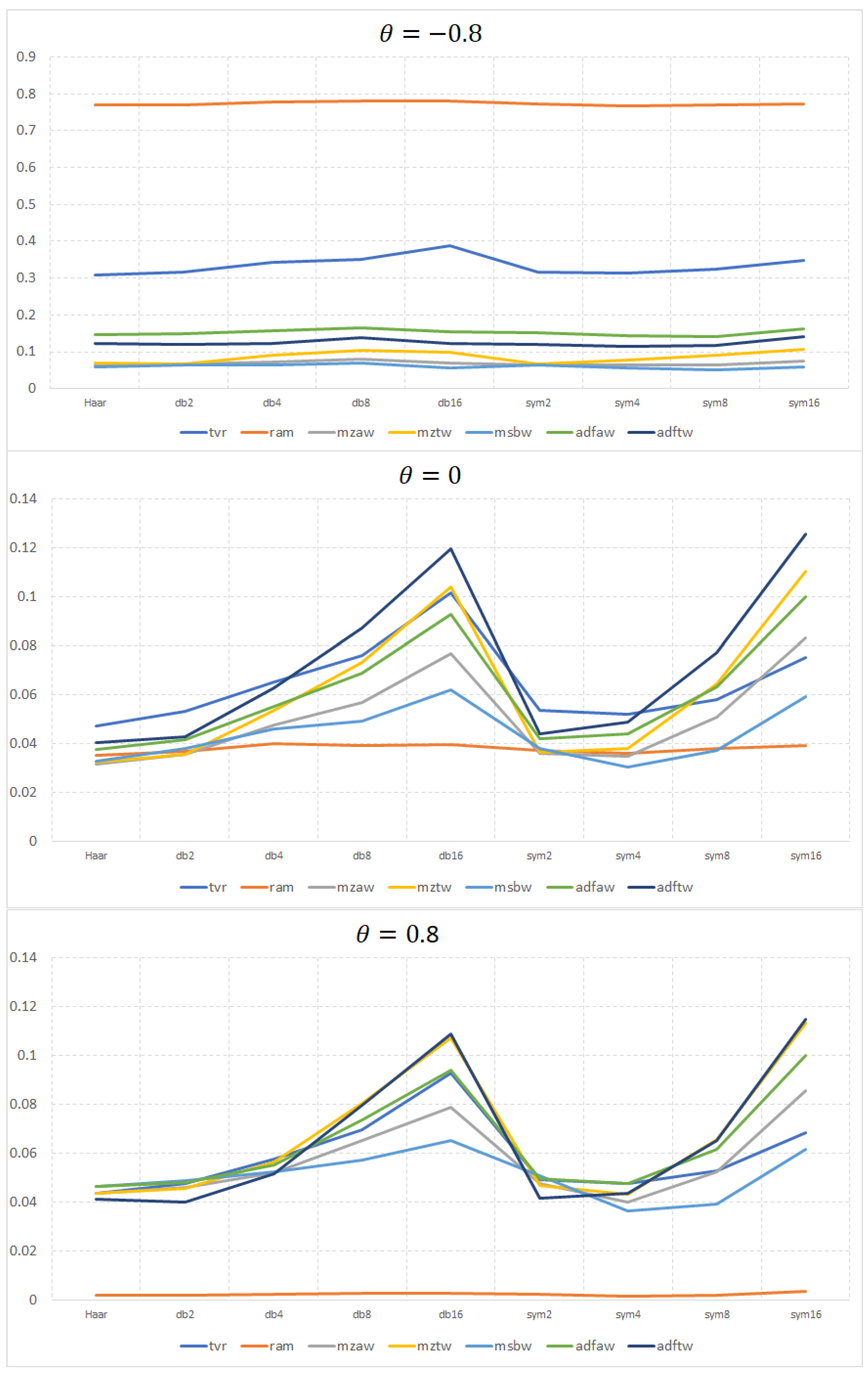
Finally, we present size properties of tests when different lengths of wavelets are selected. For the case of and GLS demeaning, Figure 1 shows sizes of tests with wavelet length between 2 and 16 for and , respectively. Results clearly show that, for and when the wavelength increases over 8, tests become significantly oversized. For , sizes of tests don’t change much with the wavelet length. These results show that tests based on smaller wavelet lengths show better size properties.
4.2. The Size-Adjusted Power Performance of the Wavelet Based Tests
In this part, we investigate the size-adjusted power properties of the wavelet based tests. We use the model in Equations (13)–(15). As in the size exercise, we utilize the same data generation and detrending algorithms, but we set as and . The results for the size-adjusted power performance of wavelet based unit root tests are summarized in Table 6, Table 7 and Table 8.
These tables demonstrate a few interesting findings. First, Fan and Gencay’s (2010) test suffers extreme power loss when and . We cannot observe conventional power curve for this test since the power is decreasing with increasing values of . This result is surprising in unit root literature. The detrending or demeaning algorithm does not alter this conclusion, but larger sample size approximately corrects this distortion. On the other hand, other tests still maintain conventional power performance. Second, detrending or demeaning slightly reduce the power of the tests for both small and large samples. Third, the tests show similar power performance in the no serial correlation case. However, we observe slightly worse power for Trokić’s (2016) test when than the other tests. Finally, when we compare M tests and ADF tests, ADF tests exhibit better performance than M tests in almost all cases.
These findings imply that there is no single dominant test by means of size and size-adjusted power. While M and ADF tests engender better size correction in problematic cases, Trokić (2016) generates more stable power properties. Moreover, the type of wavelet filter (being from the family of Daubechies or Symlets) does not matter by means of size or size-adjusted power.
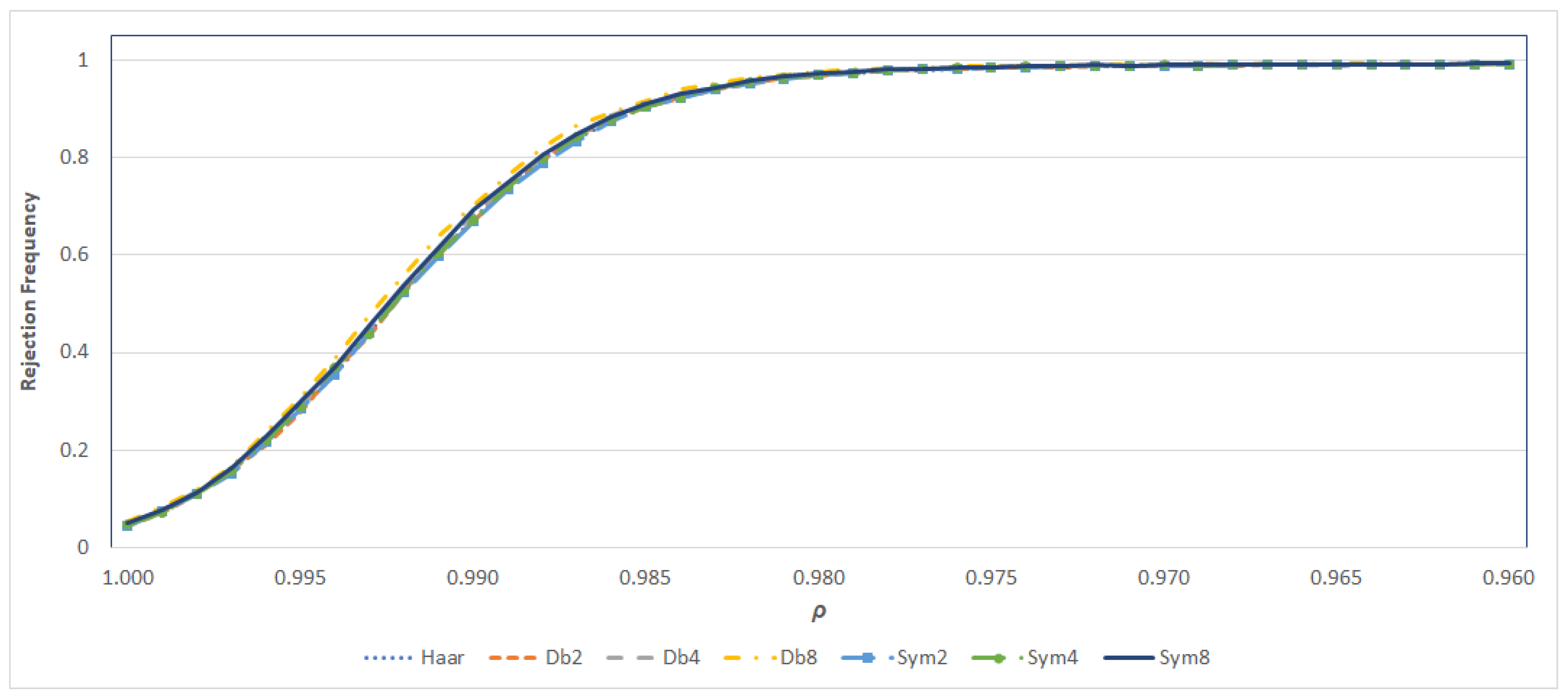
In the last two Monte Carlo exercises, we evaluate the large sample properties of the wavelet based and standard unit root tests under GLS demeaning8. First, we examine the asymptotic behaviour of the wavelet based test with different wavelet filters and lengths. In this exercise, we only consider the asymptotic power properties of the test and seven different wavelet filters, namely , , , , , and . These results, which are generated under no serial correlation and sample size 1000, are presented in Figure 2. From this figure, it is clear that wavelet type and length do not matter asymptotically.
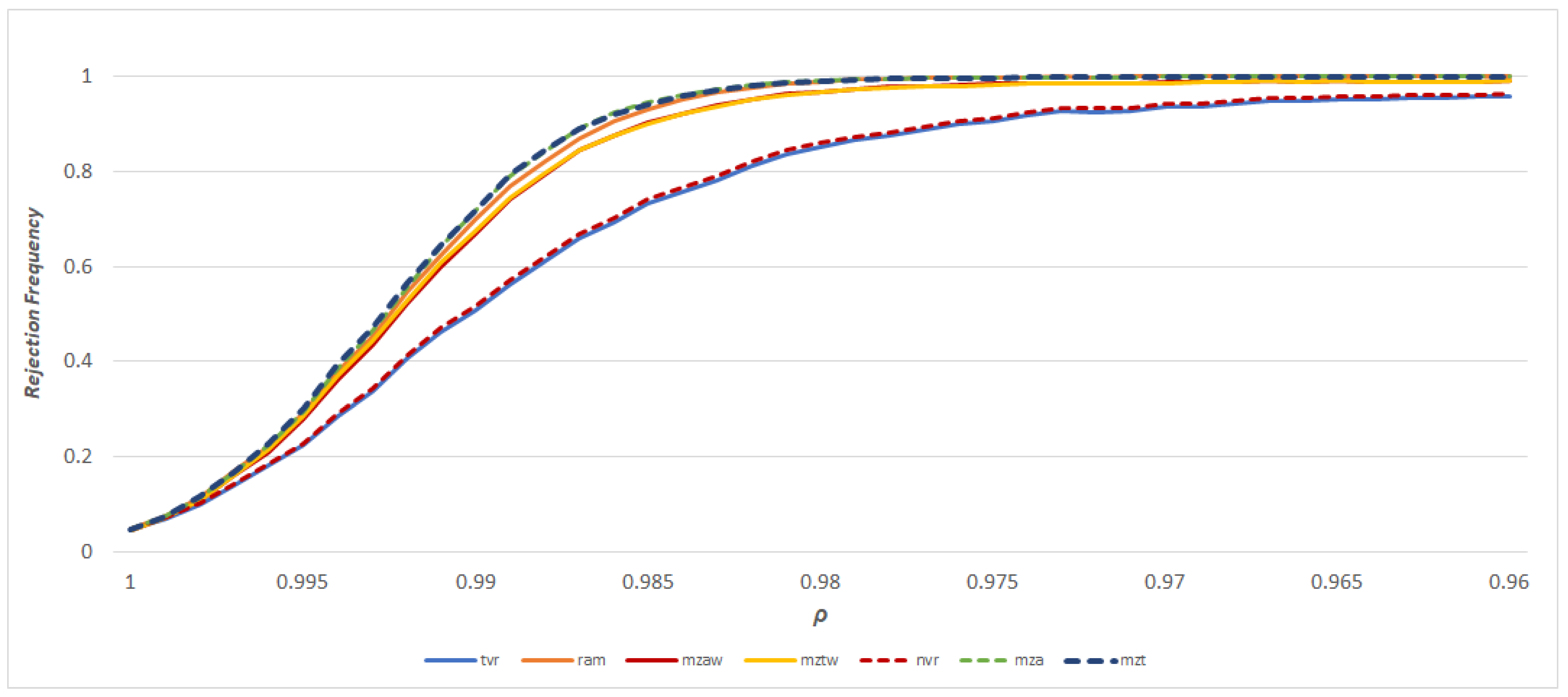
In another exercise, we compare the asymptotic power curves of the GLS demeaned standard and wavelet based tests. From these tests, we consider , , and , as the wavelet based tests, and , and as standard unit root tests. The results of the simulations, which are run with no serial correlation and sample size 1000, are given in Figure 3. The findings are twofold: (1) Nielsen’s (2009) test and its wavelet version are almost asymptotically equivalent; and (2) there are very slight deviations in other tests. However, increasing the sample size further may eliminate the difference further. On the other hand, the figure illustrates that the most powerful tests are M tests, the second rank belongs to Fan and Gencay’s (2010) test and the least powerful tests are Nielsen’s (2009) test.
5. Conclusions
In this study, we extend the results of Fan and Gencay (2010) in Ng and Perron’s (2001) framework and we provide an analysis of the application of GLS detrending in the wavelet framework.
As a result of our comparison exercise, relative to existing wavelet based unit roots, the newly proposed tests seem to be more robust to problematic innovation structures such as negative MA roots. Although all tests suffer size distortion from the presence of the negative MA innovations, in particular, M type tests are almost correctly sized. Furthermore, our tests also exhibit local power, while there is no single test that dominates the power performance contest.
We also show that the wavelet type does not matter in unit root testing. However, using higher length filters may distort the performance of wavelet based tests. Nonetheless, we can suggest length 2 or 4 wavelets for wavelet based unit root tests.
For the future work, we also consider wavelet based Johansen cointegration test using similar methodology. Recently, Eroğlu (2018) combine the Fan and Gencay (2010) and Trokić’s (2016) results with a Nielsen (2010) cointegration test. Utilizing wavelet based techniques in a Johansen cointegration test may engender a fruitful comparison. Finally, one can also consider the evaluation of the wavestrapping or other bootstrapping techniques for the wavelet based unit root tests.
Author Contributions
Both authors contributed equally to this manuscript.
Funding
This research received no external funding.
Conflicts of Interest
The authors declare no conflict of interest.
Appendix A. Proofs of the Theorems and the Lemmas
Lemma A1.
Suppose that Assumptions 1 and 2 hold and define . Under the null hypothesis of ,
where is a standard Brownian motion and is the long run variance of .
Lemma A2.
Proof of Lemma 2.
First, we decompose as where when and where when . Now, we write
Note that . This result implies that
Elliott et al. (1996) as a result converges to zero in the limit, and the convergence of the second deterministic term is shown as
Using these results, we can rewrite Equations (A1) and (A2) as:
Note that and . The second term can be written as in the limit since . Finally, we can show,
where Equation (A7) follows from the fact that . ☐
Lemma A3.
Let assumptions of Theorem 1 hold, then .
Proof of Lemma 3.
The proof of this lemma can be obtained from the consistency of , which is demonstrated in Lemma 3.5 of Chang and Park (2002) and the results of Lemma A1. First, note that , thus . Additionally, is a consistent estimator of the variance of . However, from Fan and Gencay (2010) and Trokić (2016), we know the long run variance of is given as , and then we obtain the result from Continuous Mapping Theorem (CMT) since we also have . ☐
Proof of Theorem 1.
The proof of results for the ADF test based on wavelet transformed series directly follows Chang and Park (2002). Note that the wavelet based augmented regression satisfies the same conditions as the classical ADF regression. As a result, we can use Lemmas A2 and A3 to obtain the results. The proof is the same as in Chang and Park (2002), and thus we skip the details.
The results for the wavelet based M tests follow from Lemmas A2 and A3. We simply apply CMT to reach the desired outcome. ☐
References
- Chang, Yoosoon, and Joon Y. Park. 2002. On the asymptotics of ADF tests for unit roots. Econometric Reviews 21: 431–47. [Google Scholar] [CrossRef]
- Dickey, David A., and Wayne A. Fuller. 1979. Distribution of the estimators for autoregressive time series with a unit root. Journal of the American Statistical Association 74: 427–31. [Google Scholar]
- Dickey, David A., and Wayne A. Fuller. 1981. Likelihood ratio statistics for autoregressive time series with a unit root. Econometrica 49: 1057–72. [Google Scholar] [CrossRef]
- Elliott, Graham, Thomas J. Rothenberg, and James H. Stock. 1996. Efficient Tests for an Autoregressive Unit Root. Econometrica 64: 813–36. [Google Scholar] [CrossRef]
- Eroğu, Burak. 2018. Wavelet Variance Ratio Test And Wavestrapping for the Determination of the Cointegration Rank. CEFIS Working Paper Series November 2017; Frankfurt am Main, Germany: The Center for Financial Studies. [Google Scholar]
- Fan, Yanqin, and Ramazan Gencay. 2010. Unit Root Tests with Wavelets. Econometric Theory 5: 1305–31. [Google Scholar] [CrossRef]
- Gençay, Ramazan, Faruk Selçuk, and Brandon J. Whitcher. 2001. An Introduction to Wavelets and Other Filtering Methods in Finance and Economics. Cambridge, MA, USA: Academic Press. [Google Scholar]
- Granger, Clive W. J. 1966. The typical spectral shape of an economic variable. Econometrica 34: 150–61. [Google Scholar] [CrossRef]
- Granger, Clive W. J. 1981. Some Properties of Time Series Data and Their Use in Econometric Model Specification. Journal of Econometrics 16: 121–30. [Google Scholar] [CrossRef]
- Mallat, Stephane G. 1989. A Theory for Multiresolution Signal Decomposition: The Wavelet Representation. Pattern Analysis and Machine Intelligence. IEEE Transactions 11: 674–93. [Google Scholar]
- Ng, Serena, and Pierre Perron. 2001. Lag length selection and the construction of unit root tests with good size and power. Econometrica 69: 1519–54. [Google Scholar] [CrossRef]
- Nielsen, Morten Ørregaard. 2009. A powerful Test of the Autoregressive Unit Root Hypothesis Based on a Tuning Parameter Free Statistic. Econometric Theory 25: 1515–44. [Google Scholar] [CrossRef]
- Nielsen, Morten Ørregaard. 2010. Nonparametric Cointegration Analysis of Fractional Systems with Unknown Integration Orders. Journal of Econometrics 155: 170–87. [Google Scholar] [CrossRef]
- Perron, Pierre, and Zhongjun Qu. 2007. A simple modification to improve the finite sample properties of Ng and Perron’s unit root tests. Economics Letters 94: 12–19. [Google Scholar] [CrossRef]
- Phillips, Peter C. B., and Pierre Perron. 1988. Testing for a Unit Root in Time Series Regression. Biometrika 75: 335–46. [Google Scholar] [CrossRef]
- Trokic, Mirza. 2016. Wavelet Energy Ratio Unit Root Tests. Econometric Reviews, 1–19. [Google Scholar] [CrossRef]
| 1. | The quadrature mirror relationship can be characterized by: for (Fan and Gencay 2010). |
| 2. | The results for the maximum overlap discrete wavelet transform are available upon request. |
| 3. | Similar to the results observed in the literature, we observe that GLS detrending generates better power performance than the ordinary least squares (OLS) detrending mechanism, so we use GLS detrending in this study. Results for OLS detrending are available upon request. |
| 4. | We also consider Daubechies and Symlet wavelets with different lengths, but they exhibit similar performance by means of size and size-adjusted power. |
| 5. | The results for other intermediate values of are available upon request. |
| 6. | In the simulation, we observe that, for all tests, the optimal is very close. As a result, we use the same for all tests. A similar approach is adopted by Ng and Perron (2001). The values of critical values with other significant levels are available upon request. |
| 7. | The simulations can be conducted under different ARMA innovations. These results are available upon request. Since they do not alter the findings, we skip them for brevity. |
| 8. | We also consider GLS detrending, but, for the space considerations, we do not present them. If requested, they are available from the authors. |
Figure 1.
The size comparison of tests with various wavelet lengths with sample size T = 100. Note: tvr, ram, mzaw, mztv, msbw, adfaw and adftw correspond to , , , , , , and , respectively.
Figure 1.
The size comparison of tests with various wavelet lengths with sample size T = 100. Note: tvr, ram, mzaw, mztv, msbw, adfaw and adftw correspond to , , , , , , and , respectively.

Figure 2.
Asymptotic power curves of the wavelet based with different wavelet filters under GLS demeaning. Note: Filters are defined in the text.
Figure 2.
Asymptotic power curves of the wavelet based with different wavelet filters under GLS demeaning. Note: Filters are defined in the text.

Figure 3.
Asymptotic power curves of the wavelet based and standard unit root tests under GLS demeaning. Note: and correspond to , , and , respectively. and correspond to , and which are standard unit root tests without the wavelet application, respectively.
Figure 3.
Asymptotic power curves of the wavelet based and standard unit root tests under GLS demeaning. Note: and correspond to , , and , respectively. and correspond to , and which are standard unit root tests without the wavelet application, respectively.


Table 1.
The values of and the associated critical values of the wavelet based tests at a 5% significance level.
Table 1.
The values of and the associated critical values of the wavelet based tests at a 5% significance level.
| , | , | |||
|---|---|---|---|---|
| 1 | 9.8 | −16.94 | −2.83 | 0.17 |
| 18.8 | −7.91 | −1.92 | 0.23 |
Table 2.
The empirical size of wavelet based tests with sample size = 100.
| Wavelet | |||||||||
|---|---|---|---|---|---|---|---|---|---|
| 0 | −0.8 | Haar | 0.212 | 0.729 | 0.040 | 0.046 | 0.034 | 0.085 | 0.067 |
| Db2 | 0.212 | 0.729 | 0.041 | 0.049 | 0.035 | 0.084 | 0.066 | ||
| Db4 | 0.220 | 0.729 | 0.038 | 0.047 | 0.034 | 0.086 | 0.067 | ||
| sym2 | 0.214 | 0.727 | 0.041 | 0.049 | 0.035 | 0.085 | 0.066 | ||
| sym4 | 0.207 | 0.723 | 0.040 | 0.046 | 0.033 | 0.084 | 0.065 | ||
| 0 | Haar | 0.040 | 0.046 | 0.028 | 0.030 | 0.028 | 0.031 | 0.031 | |
| Db2 | 0.041 | 0.045 | 0.029 | 0.030 | 0.030 | 0.031 | 0.031 | ||
| Db4 | 0.045 | 0.047 | 0.033 | 0.036 | 0.031 | 0.035 | 0.036 | ||
| sym2 | 0.044 | 0.046 | 0.030 | 0.031 | 0.030 | 0.033 | 0.032 | ||
| sym4 | 0.040 | 0.043 | 0.028 | 0.029 | 0.027 | 0.032 | 0.031 | ||
| 0.8 | Haar | 0.037 | 0.020 | 0.040 | 0.040 | 0.040 | 0.043 | 0.039 | |
| Db2 | 0.039 | 0.020 | 0.040 | 0.040 | 0.041 | 0.042 | 0.036 | ||
| Db4 | 0.042 | 0.020 | 0.040 | 0.043 | 0.040 | 0.040 | 0.036 | ||
| sym2 | 0.039 | 0.019 | 0.040 | 0.040 | 0.041 | 0.042 | 0.037 | ||
| sym4 | 0.038 | 0.018 | 0.036 | 0.037 | 0.034 | 0.039 | 0.034 | ||
| 1 | −0.8 | Haar | 0.227 | 0.803 | 0.035 | 0.039 | 0.031 | 0.088 | 0.074 |
| Db2 | 0.228 | 0.804 | 0.035 | 0.037 | 0.034 | 0.087 | 0.071 | ||
| Db4 | 0.241 | 0.806 | 0.043 | 0.056 | 0.034 | 0.091 | 0.073 | ||
| sym2 | 0.232 | 0.804 | 0.034 | 0.036 | 0.032 | 0.087 | 0.071 | ||
| sym4 | 0.229 | 0.802 | 0.039 | 0.046 | 0.033 | 0.089 | 0.073 | ||
| 0 | Haar | 0.048 | 0.054 | 0.033 | 0.033 | 0.033 | 0.036 | 0.035 | |
| Db2 | 0.050 | 0.053 | 0.033 | 0.033 | 0.035 | 0.037 | 0.035 | ||
| Db4 | 0.053 | 0.055 | 0.040 | 0.042 | 0.037 | 0.042 | 0.042 | ||
| sym2 | 0.051 | 0.054 | 0.034 | 0.035 | 0.035 | 0.038 | 0.037 | ||
| sym4 | 0.051 | 0.053 | 0.035 | 0.036 | 0.032 | 0.038 | 0.038 | ||
| 0.8 | Haar | 0.045 | 0.022 | 0.046 | 0.046 | 0.048 | 0.049 | 0.044 | |
| Db2 | 0.045 | 0.022 | 0.046 | 0.046 | 0.047 | 0.049 | 0.042 | ||
| Db4 | 0.050 | 0.024 | 0.050 | 0.053 | 0.048 | 0.050 | 0.044 | ||
| sym2 | 0.048 | 0.022 | 0.046 | 0.047 | 0.048 | 0.049 | 0.042 | ||
| sym4 | 0.048 | 0.022 | 0.045 | 0.046 | 0.042 | 0.048 | 0.042 | ||
| −0.8 | Haar | 0.498 | 0.999 | 0.030 | 0.032 | 0.028 | 0.113 | 0.072 | |
| Db2 | 0.501 | 0.999 | 0.031 | 0.032 | 0.030 | 0.113 | 0.069 | ||
| Db4 | 0.519 | 0.999 | 0.033 | 0.040 | 0.029 | 0.116 | 0.068 | ||
| sym2 | 0.502 | 0.999 | 0.031 | 0.032 | 0.030 | 0.116 | 0.071 | ||
| sym4 | 0.513 | 0.999 | 0.032 | 0.034 | 0.030 | 0.116 | 0.069 | ||
| 0 | Haar | 0.051 | 0.038 | 0.010 | 0.011 | 0.011 | 0.017 | 0.020 | |
| Db2 | 0.058 | 0.039 | 0.012 | 0.012 | 0.012 | 0.017 | 0.021 | ||
| Db4 | 0.064 | 0.040 | 0.015 | 0.017 | 0.014 | 0.023 | 0.029 | ||
| sym2 | 0.055 | 0.037 | 0.012 | 0.012 | 0.012 | 0.018 | 0.021 | ||
| sym4 | 0.065 | 0.041 | 0.013 | 0.014 | 0.013 | 0.021 | 0.024 | ||
| 0.8 | Haar | 0.045 | 0.021 | 0.025 | 0.026 | 0.026 | 0.032 | 0.027 | |
| Db2 | 0.049 | 0.022 | 0.025 | 0.025 | 0.026 | 0.032 | 0.024 | ||
| Db4 | 0.056 | 0.024 | 0.027 | 0.028 | 0.026 | 0.032 | 0.026 | ||
| sym2 | 0.048 | 0.022 | 0.026 | 0.026 | 0.027 | 0.032 | 0.025 | ||
| sym4 | 0.056 | 0.023 | 0.022 | 0.023 | 0.022 | 0.030 | 0.024 |
Table 3.
The empirical size of wavelet based tests with sample size = 1000.
| Wavelet | |||||||||
|---|---|---|---|---|---|---|---|---|---|
| 0 | −0.8 | Haar | 0.113 | 0.636 | 0.051 | 0.053 | 0.047 | 0.067 | 0.06 |
| Db2 | 0.114 | 0.637 | 0.053 | 0.056 | 0.049 | 0.069 | 0.062 | ||
| Db4 | 0.118 | 0.638 | 0.052 | 0.055 | 0.05 | 0.068 | 0.062 | ||
| sym2 | 0.115 | 0.638 | 0.053 | 0.056 | 0.051 | 0.069 | 0.062 | ||
| sym4 | 0.115 | 0.635 | 0.054 | 0.057 | 0.05 | 0.069 | 0.063 | ||
| 0 | Haar | 0.046 | 0.049 | 0.047 | 0.047 | 0.047 | 0.048 | 0.047 | |
| Db2 | 0.048 | 0.05 | 0.049 | 0.048 | 0.048 | 0.049 | 0.047 | ||
| Db4 | 0.05 | 0.049 | 0.048 | 0.047 | 0.047 | 0.048 | 0.045 | ||
| sym2 | 0.048 | 0.049 | 0.048 | 0.048 | 0.048 | 0.048 | 0.047 | ||
| sym4 | 0.047 | 0.048 | 0.046 | 0.046 | 0.045 | 0.046 | 0.045 | ||
| 0.8 | Haar | 0.045 | 0.04 | 0.044 | 0.045 | 0.045 | 0.045 | 0.044 | |
| Db2 | 0.048 | 0.041 | 0.046 | 0.047 | 0.046 | 0.047 | 0.045 | ||
| Db4 | 0.05 | 0.041 | 0.048 | 0.048 | 0.047 | 0.048 | 0.045 | ||
| sym2 | 0.047 | 0.04 | 0.045 | 0.045 | 0.046 | 0.046 | 0.044 | ||
| sym4 | 0.047 | 0.041 | 0.046 | 0.047 | 0.046 | 0.047 | 0.045 | ||
| 1 | −0.8 | Haar | 0.112 | 0.651 | 0.049 | 0.051 | 0.047 | 0.067 | 0.062 |
| Db2 | 0.114 | 0.651 | 0.046 | 0.048 | 0.046 | 0.067 | 0.061 | ||
| Db4 | 0.112 | 0.652 | 0.052 | 0.056 | 0.048 | 0.068 | 0.062 | ||
| sym2 | 0.108 | 0.652 | 0.047 | 0.048 | 0.045 | 0.066 | 0.061 | ||
| sym4 | 0.111 | 0.652 | 0.049 | 0.051 | 0.046 | 0.065 | 0.06 | ||
| 0 | Haar | 0.047 | 0.049 | 0.048 | 0.048 | 0.048 | 0.049 | 0.048 | |
| Db2 | 0.048 | 0.048 | 0.047 | 0.047 | 0.047 | 0.047 | 0.046 | ||
| Db4 | 0.048 | 0.051 | 0.048 | 0.05 | 0.048 | 0.049 | 0.047 | ||
| sym2 | 0.047 | 0.05 | 0.049 | 0.048 | 0.048 | 0.049 | 0.047 | ||
| sym4 | 0.048 | 0.05 | 0.047 | 0.047 | 0.047 | 0.047 | 0.046 | ||
| 0.8 | Haar | 0.046 | 0.041 | 0.046 | 0.046 | 0.046 | 0.046 | 0.044 | |
| Db2 | 0.048 | 0.041 | 0.045 | 0.046 | 0.046 | 0.046 | 0.044 | ||
| Db4 | 0.047 | 0.041 | 0.047 | 0.048 | 0.047 | 0.047 | 0.044 | ||
| sym2 | 0.047 | 0.041 | 0.046 | 0.046 | 0.046 | 0.047 | 0.044 | ||
| sym4 | 0.047 | 0.041 | 0.046 | 0.046 | 0.046 | 0.047 | 0.044 | ||
| −0.8 | Haar | 0.268 | 0.994 | 0.031 | 0.032 | 0.029 | 0.074 | 0.056 | |
| Db2 | 0.267 | 0.994 | 0.03 | 0.031 | 0.03 | 0.074 | 0.056 | ||
| Db4 | 0.27 | 0.994 | 0.033 | 0.038 | 0.03 | 0.075 | 0.056 | ||
| sym2 | 0.267 | 0.994 | 0.032 | 0.033 | 0.031 | 0.075 | 0.058 | ||
| sym4 | 0.272 | 0.994 | 0.032 | 0.034 | 0.03 | 0.073 | 0.056 | ||
| 0 | Haar | 0.062 | 0.048 | 0.041 | 0.041 | 0.041 | 0.044 | 0.042 | |
| Db2 | 0.063 | 0.049 | 0.043 | 0.043 | 0.043 | 0.046 | 0.042 | ||
| Db4 | 0.065 | 0.049 | 0.043 | 0.044 | 0.043 | 0.045 | 0.041 | ||
| sym2 | 0.063 | 0.049 | 0.043 | 0.043 | 0.043 | 0.046 | 0.042 | ||
| sym4 | 0.068 | 0.051 | 0.044 | 0.044 | 0.043 | 0.046 | 0.042 | ||
| 0.8 | Haar | 0.06 | 0.028 | 0.041 | 0.042 | 0.042 | 0.044 | 0.039 | |
| Db2 | 0.06 | 0.028 | 0.04 | 0.041 | 0.04 | 0.043 | 0.037 | ||
| Db4 | 0.065 | 0.028 | 0.042 | 0.043 | 0.042 | 0.043 | 0.036 | ||
| sym2 | 0.06 | 0.028 | 0.041 | 0.041 | 0.041 | 0.044 | 0.038 | ||
| sym4 | 0.065 | 0.029 | 0.042 | 0.043 | 0.041 | 0.045 | 0.038 |
Table 4.
The size comparison of the standard and wavelet based unit root tests under GLS demeaning.
| Wavelet Based Tests | |||||||
|---|---|---|---|---|---|---|---|
| T | |||||||
| 100 | −0.8 | 0.315 | 0.066 | 0.068 | 0.064 | 0.150 | 0.121 |
| 0 | 0.053 | 0.037 | 0.036 | 0.036 | 0.042 | 0.043 | |
| 0.8 | 0.048 | 0.046 | 0.046 | 0.049 | 0.048 | 0.040 | |
| 1000 | −0.8 | 0.113 | 0.047 | 0.048 | 0.047 | 0.067 | 0.062 |
| 0 | 0.048 | 0.050 | 0.048 | 0.048 | 0.049 | 0.047 | |
| 0.8 | 0.045 | 0.039 | 0.044 | 0.045 | 0.045 | 0.043 | |
| Standard Tests | |||||||
| T | |||||||
| 100 | −0.8 | 0.582 | 0.037 | 0.039 | 0.035 | 0.162 | 0.119 |
| 0 | 0.069 | 0.047 | 0.048 | 0.047 | 0.054 | 0.056 | |
| 0.8 | 0.054 | 0.071 | 0.070 | 0.072 | 0.072 | 0.043 | |
| 1000 | −0.8 | 0.186 | 0.041 | 0.042 | 0.039 | 0.080 | 0.074 |
| 0 | 0.050 | 0.048 | 0.048 | 0.049 | 0.049 | 0.049 | |
| 0.8 | 0.047 | 0.053 | 0.053 | 0.053 | 0.054 | 0.048 | |
Table 5.
The size comparison of the OLS and GLS demeaning with sample size T = 100.
| GLS Demeaning | ||||||||
|---|---|---|---|---|---|---|---|---|
| Wavelet | ||||||||
| Haar | −0.8 | 0.307 | 0.771 | 0.065 | 0.071 | 0.059 | 0.147 | 0.123 |
| 0 | 0.047 | 0.035 | 0.032 | 0.033 | 0.033 | 0.038 | 0.041 | |
| 0.8 | 0.044 | 0.002 | 0.044 | 0.044 | 0.047 | 0.047 | 0.041 | |
| db2 | −0.8 | 0.315 | 0.771 | 0.066 | 0.068 | 0.064 | 0.150 | 0.121 |
| 0 | 0.053 | 0.037 | 0.036 | 0.036 | 0.038 | 0.042 | 0.043 | |
| 0.8 | 0.048 | 0.002 | 0.046 | 0.046 | 0.049 | 0.048 | 0.040 | |
| sym2 | −0.8 | 0.317 | 0.772 | 0.065 | 0.067 | 0.064 | 0.151 | 0.120 |
| 0 | 0.054 | 0.037 | 0.036 | 0.037 | 0.038 | 0.042 | 0.044 | |
| 0.8 | 0.049 | 0.002 | 0.048 | 0.047 | 0.051 | 0.050 | 0.042 | |
| OLS demeaning | ||||||||
| Wavelet | ||||||||
| Haar | −0.8 | 0.423 | 0.999 | 0.073 | 0.063 | 0.077 | 0.184 | 0.105 |
| 0 | 0.017 | 0.020 | 0.011 | 0.021 | 0.013 | 0.017 | 0.033 | |
| 0.8 | 0.013 | 0.000 | 0.015 | 0.023 | 0.019 | 0.020 | 0.029 | |
| db2 | −0.8 | 0.423 | 0.999 | 0.077 | 0.068 | 0.081 | 0.190 | 0.119 |
| 0 | 0.018 | 0.018 | 0.010 | 0.014 | 0.013 | 0.016 | 0.028 | |
| 0.8 | 0.014 | 0.000 | 0.014 | 0.018 | 0.020 | 0.019 | 0.026 | |
| sym2 | −0.8 | 0.432 | 0.999 | 0.078 | 0.069 | 0.081 | 0.192 | 0.119 |
| 0 | 0.019 | 0.019 | 0.010 | 0.015 | 0.014 | 0.017 | 0.031 | |
| 0.8 | 0.015 | 0.000 | 0.015 | 0.018 | 0.021 | 0.020 | 0.028 | |
Table 6.
The size-adjusted power of wavelet based tests.
| T | Wavelet | ||||||||||
|---|---|---|---|---|---|---|---|---|---|---|---|
| 100 | 0 | −0.8 | Haar | 0.99 | 0.109 | 0.104 | 0.109 | 0.111 | 0.104 | 0.111 | 0.111 |
| 0.9 | 0.988 | 0.073 | 0.523 | 0.537 | 0.507 | 0.769 | 0.640 | ||||
| Db2 | 0.99 | 0.115 | 0.105 | 0.108 | 0.109 | 0.105 | 0.113 | 0.113 | |||
| 0.9 | 0.989 | 0.073 | 0.520 | 0.535 | 0.505 | 0.772 | 0.643 | ||||
| Db4 | 0.99 | 0.113 | 0.104 | 0.110 | 0.111 | 0.106 | 0.115 | 0.115 | |||
| 0.9 | 0.989 | 0.072 | 0.516 | 0.521 | 0.508 | 0.781 | 0.655 | ||||
| sym2 | 0.99 | 0.114 | 0.107 | 0.109 | 0.111 | 0.104 | 0.112 | 0.113 | |||
| 0.9 | 0.989 | 0.075 | 0.524 | 0.539 | 0.507 | 0.773 | 0.645 | ||||
| sym4 | 0.99 | 0.117 | 0.109 | 0.111 | 0.109 | 0.109 | 0.114 | 0.114 | |||
| 0.9 | 0.991 | 0.078 | 0.522 | 0.530 | 0.512 | 0.776 | 0.641 | ||||
| 0 | Haar | 0.99 | 0.101 | 0.110 | 0.110 | 0.112 | 0.101 | 0.111 | 0.115 | ||
| 0.9 | 0.884 | 0.980 | 0.859 | 0.859 | 0.843 | 0.903 | 0.870 | ||||
| Db2 | 0.99 | 0.103 | 0.113 | 0.110 | 0.114 | 0.104 | 0.113 | 0.115 | |||
| 0.9 | 0.889 | 0.982 | 0.853 | 0.854 | 0.839 | 0.901 | 0.866 | ||||
| Db4 | 0.99 | 0.101 | 0.112 | 0.114 | 0.116 | 0.106 | 0.114 | 0.118 | |||
| 0.9 | 0.889 | 0.981 | 0.854 | 0.856 | 0.837 | 0.896 | 0.856 | ||||
| sym2 | 0.99 | 0.102 | 0.112 | 0.112 | 0.113 | 0.105 | 0.113 | 0.116 | |||
| 0.9 | 0.883 | 0.979 | 0.853 | 0.854 | 0.838 | 0.900 | 0.865 | ||||
| sym4 | 0.99 | 0.106 | 0.115 | 0.117 | 0.118 | 0.111 | 0.117 | 0.120 | |||
| 0.9 | 0.898 | 0.982 | 0.852 | 0.851 | 0.844 | 0.897 | 0.857 | ||||
| 0.8 | Haar | 0.99 | 0.105 | 0.114 | 0.113 | 0.115 | 0.108 | 0.115 | 0.117 | ||
| 0.9 | 0.873 | 0.952 | 0.789 | 0.790 | 0.767 | 0.844 | 0.811 | ||||
| Db2 | 0.99 | 0.103 | 0.111 | 0.111 | 0.112 | 0.105 | 0.113 | 0.114 | |||
| 0.9 | 0.875 | 0.950 | 0.790 | 0.791 | 0.771 | 0.851 | 0.817 | ||||
| Db4 | 0.99 | 0.103 | 0.113 | 0.113 | 0.115 | 0.107 | 0.115 | 0.118 | |||
| 0.9 | 0.879 | 0.951 | 0.805 | 0.808 | 0.781 | 0.860 | 0.824 | ||||
| sym2 | 0.99 | 0.104 | 0.114 | 0.111 | 0.113 | 0.106 | 0.115 | 0.115 | |||
| 0.9 | 0.878 | 0.951 | 0.791 | 0.791 | 0.770 | 0.851 | 0.818 | ||||
| sym4 | 0.99 | 0.106 | 0.115 | 0.113 | 0.115 | 0.109 | 0.114 | 0.115 | |||
| 0.9 | 0.886 | 0.954 | 0.801 | 0.797 | 0.790 | 0.855 | 0.813 | ||||
| 1 | −0.8 | Haar | 0.99 | 0.093 | 0.087 | 0.091 | 0.091 | 0.088 | 0.093 | 0.090 | |
| 0.9 | 0.371 | 0.017 | 0.148 | 0.151 | 0.143 | 0.237 | 0.189 | ||||
| Db2 | 0.99 | 0.094 | 0.086 | 0.090 | 0.090 | 0.086 | 0.095 | 0.092 | |||
| 0.9 | 0.377 | 0.016 | 0.148 | 0.149 | 0.145 | 0.240 | 0.193 | ||||
| Db4 | 0.99 | 0.092 | 0.086 | 0.086 | 0.086 | 0.086 | 0.090 | 0.088 | |||
| 0.9 | 0.373 | 0.016 | 0.147 | 0.156 | 0.144 | 0.242 | 0.197 | ||||
| sym2 | 0.99 | 0.095 | 0.087 | 0.092 | 0.093 | 0.089 | 0.094 | 0.093 | |||
| 0.9 | 0.374 | 0.017 | 0.149 | 0.149 | 0.146 | 0.238 | 0.193 | ||||
| sym4 | 0.99 | 0.095 | 0.087 | 0.091 | 0.089 | 0.089 | 0.093 | 0.090 | |||
| 0.9 | 0.377 | 0.017 | 0.152 | 0.154 | 0.149 | 0.243 | 0.194 | ||||
| 0 | Haar | 0.99 | 0.101 | 0.111 | 0.108 | 0.110 | 0.102 | 0.110 | 0.114 | ||
| 0.9 | 0.728 | 0.895 | 0.776 | 0.775 | 0.756 | 0.820 | 0.791 | ||||
| Db2 | 0.99 | 0.100 | 0.114 | 0.111 | 0.113 | 0.104 | 0.112 | 0.116 | |||
| 0.9 | 0.735 | 0.900 | 0.775 | 0.774 | 0.754 | 0.819 | 0.787 | ||||
| Db4 | 0.99 | 0.104 | 0.113 | 0.109 | 0.111 | 0.103 | 0.111 | 0.114 | |||
| 0.9 | 0.747 | 0.899 | 0.775 | 0.779 | 0.754 | 0.818 | 0.776 | ||||
| sym2 | 0.99 | 0.103 | 0.112 | 0.108 | 0.110 | 0.102 | 0.109 | 0.112 | |||
| 0.9 | 0.737 | 0.898 | 0.771 | 0.771 | 0.751 | 0.818 | 0.785 | ||||
| sym4 | 0.99 | 0.107 | 0.115 | 0.112 | 0.113 | 0.108 | 0.114 | 0.114 | |||
| 0.9 | 0.747 | 0.900 | 0.765 | 0.761 | 0.756 | 0.812 | 0.768 | ||||
| 0.8 | Haar | 0.99 | 0.102 | 0.111 | 0.110 | 0.112 | 0.103 | 0.112 | 0.114 | ||
| 0.9 | 0.839 | 0.927 | 0.746 | 0.749 | 0.718 | 0.806 | 0.778 | ||||
| Db2 | 0.99 | 0.104 | 0.112 | 0.110 | 0.112 | 0.107 | 0.113 | 0.112 | |||
| 0.9 | 0.847 | 0.928 | 0.751 | 0.752 | 0.730 | 0.814 | 0.782 | ||||
| Db4 | 0.99 | 0.103 | 0.111 | 0.110 | 0.111 | 0.105 | 0.113 | 0.114 | |||
| 0.9 | 0.854 | 0.928 | 0.773 | 0.776 | 0.745 | 0.829 | 0.793 | ||||
| sym2 | 0.99 | 0.102 | 0.112 | 0.112 | 0.114 | 0.104 | 0.114 | 0.118 | |||
| 0.9 | 0.845 | 0.927 | 0.753 | 0.754 | 0.724 | 0.814 | 0.786 | ||||
| sym4 | 0.99 | 0.103 | 0.110 | 0.108 | 0.110 | 0.106 | 0.110 | 0.112 | |||
| 0.9 | 0.858 | 0.930 | 0.763 | 0.759 | 0.754 | 0.819 | 0.779 |
Table 7.
The size-adjusted power of wavelet based unit root tests, continued.
| T | Wavelet | ||||||||||
|---|---|---|---|---|---|---|---|---|---|---|---|
| 100 | −0.8 | Haar | 0.99 | 0.058 | 0.055 | 0.057 | 0.057 | 0.057 | 0.058 | 0.057 | |
| 0.9 | 0.400 | 0.026 | 0.162 | 0.163 | 0.161 | 0.229 | 0.182 | ||||
| Db2 | 0.99 | 0.060 | 0.053 | 0.057 | 0.058 | 0.058 | 0.058 | 0.058 | |||
| 0.9 | 0.411 | 0.024 | 0.161 | 0.161 | 0.160 | 0.229 | 0.184 | ||||
| Db4 | 0.99 | 0.060 | 0.054 | 0.055 | 0.055 | 0.055 | 0.057 | 0.056 | |||
| 0.9 | 0.405 | 0.024 | 0.159 | 0.162 | 0.158 | 0.229 | 0.184 | ||||
| sym2 | 0.99 | 0.058 | 0.054 | 0.056 | 0.056 | 0.055 | 0.056 | 0.056 | |||
| 0.9 | 0.401 | 0.024 | 0.160 | 0.161 | 0.159 | 0.225 | 0.180 | ||||
| sym4 | 0.99 | 0.057 | 0.053 | 0.056 | 0.056 | 0.057 | 0.058 | 0.057 | |||
| 0.9 | 0.407 | 0.024 | 0.165 | 0.164 | 0.165 | 0.233 | 0.186 | ||||
| 0 | Haar | 0.99 | 0.061 | 0.061 | 0.059 | 0.059 | 0.058 | 0.060 | 0.061 | ||
| 0.9 | 0.646 | 0.805 | 0.611 | 0.613 | 0.595 | 0.648 | 0.648 | ||||
| Db2 | 0.99 | 0.060 | 0.061 | 0.061 | 0.061 | 0.061 | 0.061 | 0.062 | |||
| 0.9 | 0.640 | 0.800 | 0.612 | 0.616 | 0.599 | 0.649 | 0.646 | ||||
| Db4 | 0.99 | 0.059 | 0.060 | 0.059 | 0.059 | 0.058 | 0.060 | 0.060 | |||
| 0.9 | 0.648 | 0.804 | 0.627 | 0.628 | 0.613 | 0.662 | 0.636 | ||||
| sym2 | 0.99 | 0.061 | 0.062 | 0.060 | 0.061 | 0.059 | 0.061 | 0.060 | |||
| 0.9 | 0.644 | 0.804 | 0.611 | 0.616 | 0.597 | 0.650 | 0.644 | ||||
| sym4 | 0.99 | 0.060 | 0.060 | 0.059 | 0.059 | 0.059 | 0.060 | 0.060 | |||
| 0.9 | 0.650 | 0.802 | 0.617 | 0.614 | 0.613 | 0.652 | 0.631 | ||||
| 0.8 | Haar | 0.99 | 0.059 | 0.059 | 0.058 | 0.058 | 0.058 | 0.059 | 0.058 | ||
| 0.9 | 0.670 | 0.672 | 0.365 | 0.373 | 0.345 | 0.430 | 0.476 | ||||
| Db2 | 0.99 | 0.060 | 0.060 | 0.058 | 0.059 | 0.058 | 0.060 | 0.060 | |||
| 0.9 | 0.676 | 0.667 | 0.398 | 0.407 | 0.381 | 0.471 | 0.515 | ||||
| Db4 | 0.99 | 0.058 | 0.058 | 0.058 | 0.058 | 0.058 | 0.059 | 0.060 | |||
| 0.9 | 0.679 | 0.665 | 0.446 | 0.459 | 0.423 | 0.517 | 0.552 | ||||
| sym2 | 0.99 | 0.059 | 0.058 | 0.054 | 0.055 | 0.053 | 0.055 | 0.057 | |||
| 0.9 | 0.678 | 0.668 | 0.391 | 0.401 | 0.374 | 0.463 | 0.513 | ||||
| sym4 | 0.99 | 0.060 | 0.060 | 0.058 | 0.059 | 0.058 | 0.059 | 0.059 | |||
| 0.9 | 0.678 | 0.675 | 0.452 | 0.454 | 0.444 | 0.510 | 0.531 | ||||
| 1000 | 0 | −0.8 | Haar | 0.99 | 0.621 | 0.699 | 0.650 | 0.654 | 0.625 | 0.677 | 0.675 |
| 0.9 | 1.000 | 1.000 | 0.978 | 0.979 | 0.973 | 1.000 | 0.999 | ||||
| Db2 | 0.99 | 0.626 | 0.696 | 0.650 | 0.652 | 0.629 | 0.680 | 0.674 | |||
| 0.9 | 1.000 | 0.999 | 0.977 | 0.977 | 0.973 | 1.000 | 0.999 | ||||
| Db4 | 0.99 | 0.627 | 0.703 | 0.650 | 0.647 | 0.631 | 0.683 | 0.677 | |||
| 0.9 | 1.000 | 1.000 | 0.974 | 0.971 | 0.972 | 1.000 | 0.999 | ||||
| sym2 | 0.99 | 0.622 | 0.697 | 0.645 | 0.645 | 0.620 | 0.676 | 0.670 | |||
| 0.9 | 1.000 | 0.999 | 0.977 | 0.977 | 0.972 | 1.000 | 0.999 | ||||
| sym4 | 0.99 | 0.626 | 0.699 | 0.641 | 0.645 | 0.623 | 0.671 | 0.664 | |||
| 0.9 | 1.000 | 1.000 | 0.976 | 0.976 | 0.972 | 1.000 | 0.999 | ||||
| 0 | Haar | 0.99 | 0.523 | 0.704 | 0.707 | 0.711 | 0.680 | 0.711 | 0.711 | ||
| 0.9 | 1.000 | 1.000 | 0.999 | 0.998 | 0.999 | 1.000 | 0.999 | ||||
| Db2 | 0.99 | 0.526 | 0.707 | 0.707 | 0.707 | 0.684 | 0.709 | 0.707 | |||
| 0.9 | 1.000 | 1.000 | 0.999 | 0.999 | 0.999 | 1.000 | 0.999 | ||||
| Db4 | 0.99 | 0.528 | 0.711 | 0.712 | 0.718 | 0.686 | 0.715 | 0.717 | |||
| 0.9 | 1.000 | 1.000 | 0.999 | 0.999 | 0.999 | 1.000 | 0.999 | ||||
| sym2 | 0.99 | 0.523 | 0.711 | 0.711 | 0.712 | 0.682 | 0.714 | 0.712 | |||
| 0.9 | 1.000 | 1.000 | 0.999 | 0.998 | 0.999 | 1.000 | 0.999 | ||||
| sym4 | 0.99 | 0.533 | 0.716 | 0.714 | 0.714 | 0.690 | 0.717 | 0.715 | |||
| 0.9 | 1.000 | 1.000 | 0.999 | 0.999 | 0.999 | 1.000 | 0.999 | ||||
| 0.8 | Haar | 0.99 | 0.527 | 0.703 | 0.705 | 0.707 | 0.679 | 0.708 | 0.708 | ||
| 0.9 | 1.000 | 1.000 | 0.999 | 0.999 | 0.999 | 1.000 | 0.999 | ||||
| Db2 | 0.99 | 0.524 | 0.704 | 0.701 | 0.703 | 0.674 | 0.704 | 0.704 | |||
| 0.9 | 1.000 | 1.000 | 0.999 | 0.999 | 0.999 | 1.000 | 0.999 | ||||
| Db4 | 0.99 | 0.519 | 0.697 | 0.689 | 0.695 | 0.665 | 0.694 | 0.697 | |||
| 0.9 | 1.000 | 1.000 | 0.999 | 0.999 | 0.999 | 1.000 | 0.999 | ||||
| sym2 | 0.99 | 0.522 | 0.709 | 0.706 | 0.710 | 0.678 | 0.709 | 0.711 | |||
| 0.9 | 1.000 | 1.000 | 0.999 | 0.999 | 0.999 | 1.000 | 0.999 | ||||
| sym4 | 0.99 | 0.525 | 0.702 | 0.694 | 0.694 | 0.668 | 0.696 | 0.696 | |||
| 0.9 | 1.000 | 1.000 | 0.999 | 0.998 | 0.999 | 1.000 | 0.999 |
Table 8.
The size-adjusted power of wavelet based unit root tests, continued.
| T | Wavelet | ||||||||||
|---|---|---|---|---|---|---|---|---|---|---|---|
| 1000 | 1 | −0.8 | Haar | 0.99 | 0.391 | 0.447 | 0.454 | 0.456 | 0.438 | 0.474 | 0.471 |
| 0.9 | 0.551 | 0.429 | 0.248 | 0.255 | 0.238 | 0.433 | 0.413 | ||||
| Db2 | 0.99 | 0.387 | 0.444 | 0.455 | 0.457 | 0.436 | 0.473 | 0.469 | |||
| 0.9 | 0.554 | 0.429 | 0.245 | 0.248 | 0.238 | 0.434 | 0.414 | ||||
| Db4 | 0.99 | 0.393 | 0.448 | 0.455 | 0.454 | 0.439 | 0.477 | 0.472 | |||
| 0.9 | 0.554 | 0.430 | 0.250 | 0.266 | 0.238 | 0.435 | 0.416 | ||||
| sym2 | 0.99 | 0.397 | 0.455 | 0.461 | 0.460 | 0.443 | 0.479 | 0.474 | |||
| 0.9 | 0.557 | 0.437 | 0.246 | 0.249 | 0.240 | 0.436 | 0.416 | ||||
| sym4 | 0.99 | 0.395 | 0.452 | 0.456 | 0.458 | 0.440 | 0.474 | 0.467 | |||
| 0.9 | 0.556 | 0.435 | 0.254 | 0.264 | 0.242 | 0.437 | 0.416 | ||||
| 0 | Haar | 0.99 | 0.514 | 0.698 | 0.694 | 0.694 | 0.668 | 0.697 | 0.694 | ||
| 0.9 | 0.950 | 1.000 | 0.948 | 0.948 | 0.942 | 0.982 | 0.972 | ||||
| Db2 | 0.99 | 0.521 | 0.702 | 0.699 | 0.699 | 0.673 | 0.703 | 0.699 | |||
| 0.9 | 0.954 | 0.999 | 0.951 | 0.950 | 0.945 | 0.983 | 0.974 | ||||
| Db4 | 0.99 | 0.519 | 0.694 | 0.697 | 0.699 | 0.670 | 0.701 | 0.697 | |||
| 0.9 | 0.953 | 0.999 | 0.953 | 0.954 | 0.945 | 0.983 | 0.973 | ||||
| sym2 | 0.99 | 0.518 | 0.690 | 0.691 | 0.696 | 0.666 | 0.695 | 0.695 | |||
| 0.9 | 0.952 | 0.999 | 0.948 | 0.948 | 0.942 | 0.982 | 0.972 | ||||
| sym4 | 0.99 | 0.516 | 0.693 | 0.692 | 0.695 | 0.668 | 0.695 | 0.694 | |||
| 0.9 | 0.953 | 1.000 | 0.950 | 0.951 | 0.945 | 0.983 | 0.973 | ||||
| 0.8 | Haar | 0.99 | 0.529 | 0.699 | 0.704 | 0.706 | 0.673 | 0.707 | 0.706 | ||
| 0.9 | 0.998 | 1.000 | 0.993 | 0.992 | 0.991 | 0.999 | 0.998 | ||||
| Db2 | 0.99 | 0.526 | 0.697 | 0.696 | 0.697 | 0.667 | 0.700 | 0.700 | |||
| 0.9 | 0.998 | 1.000 | 0.992 | 0.992 | 0.991 | 0.999 | 0.998 | ||||
| Db4 | 0.99 | 0.530 | 0.699 | 0.694 | 0.697 | 0.665 | 0.698 | 0.699 | |||
| 0.9 | 0.998 | 1.000 | 0.994 | 0.994 | 0.992 | 0.999 | 0.998 | ||||
| sym2 | 0.99 | 0.526 | 0.698 | 0.696 | 0.701 | 0.669 | 0.700 | 0.702 | |||
| 0.9 | 0.998 | 1.000 | 0.993 | 0.992 | 0.991 | 0.999 | 0.998 | ||||
| sym4 | 0.99 | 0.529 | 0.695 | 0.689 | 0.689 | 0.665 | 0.691 | 0.690 | |||
| 0.9 | 0.998 | 1.000 | 0.993 | 0.993 | 0.993 | 0.999 | 0.998 | ||||
| −0.8 | Haar | 0.99 | 0.246 | 0.255 | 0.218 | 0.220 | 0.215 | 0.234 | 0.228 | ||
| 0.9 | 0.796 | 0.607 | 0.261 | 0.264 | 0.257 | 0.549 | 0.483 | ||||
| Db2 | 0.99 | 0.242 | 0.250 | 0.213 | 0.214 | 0.211 | 0.231 | 0.224 | |||
| 0.9 | 0.793 | 0.604 | 0.257 | 0.259 | 0.255 | 0.546 | 0.479 | ||||
| Db4 | 0.99 | 0.240 | 0.256 | 0.214 | 0.215 | 0.212 | 0.232 | 0.225 | |||
| 0.9 | 0.792 | 0.609 | 0.257 | 0.267 | 0.253 | 0.543 | 0.478 | ||||
| sym2 | 0.99 | 0.235 | 0.248 | 0.208 | 0.210 | 0.207 | 0.225 | 0.221 | |||
| 0.9 | 0.793 | 0.599 | 0.255 | 0.257 | 0.253 | 0.542 | 0.475 | ||||
| sym4 | 0.99 | 0.238 | 0.256 | 0.218 | 0.218 | 0.214 | 0.235 | 0.228 | |||
| 0.9 | 0.794 | 0.613 | 0.261 | 0.263 | 0.258 | 0.550 | 0.485 | ||||
| 0 | Haar | 0.99 | 0.269 | 0.302 | 0.291 | 0.293 | 0.286 | 0.293 | 0.293 | ||
| 0.9 | 0.997 | 1.000 | 0.941 | 0.942 | 0.940 | 0.992 | 0.968 | ||||
| Db2 | 0.99 | 0.260 | 0.293 | 0.278 | 0.281 | 0.274 | 0.280 | 0.282 | |||
| 0.9 | 0.997 | 1.000 | 0.938 | 0.938 | 0.937 | 0.991 | 0.966 | ||||
| Db4 | 0.99 | 0.266 | 0.292 | 0.280 | 0.283 | 0.276 | 0.281 | 0.283 | |||
| 0.9 | 0.998 | 1.000 | 0.943 | 0.945 | 0.940 | 0.991 | 0.968 | ||||
| sym2 | 0.99 | 0.262 | 0.292 | 0.281 | 0.281 | 0.275 | 0.283 | 0.283 | |||
| 0.9 | 0.998 | 1.000 | 0.938 | 0.938 | 0.937 | 0.992 | 0.967 | ||||
| sym4 | 0.99 | 0.259 | 0.290 | 0.275 | 0.278 | 0.269 | 0.277 | 0.277 | |||
| 0.9 | 0.997 | 1.000 | 0.941 | 0.941 | 0.939 | 0.992 | 0.967 | ||||
| 0.8 | Haar | 0.99 | 0.267 | 0.292 | 0.281 | 0.285 | 0.276 | 0.283 | 0.284 | ||
| 0.9 | 0.999 | 1.000 | 0.970 | 0.970 | 0.970 | 0.998 | 0.987 | ||||
| Db2 | 0.99 | 0.266 | 0.289 | 0.280 | 0.280 | 0.273 | 0.283 | 0.283 | |||
| 0.9 | 0.999 | 1.000 | 0.971 | 0.970 | 0.971 | 0.998 | 0.988 | ||||
| Db4 | 0.99 | 0.262 | 0.285 | 0.277 | 0.279 | 0.271 | 0.279 | 0.282 | |||
| 0.9 | 0.999 | 1.000 | 0.971 | 0.972 | 0.970 | 0.998 | 0.989 | ||||
| sym2 | 0.99 | 0.260 | 0.281 | 0.275 | 0.279 | 0.268 | 0.277 | 0.278 | |||
| 0.9 | 0.999 | 1.000 | 0.971 | 0.970 | 0.970 | 0.998 | 0.989 | ||||
| sym4 | 0.99 | 0.261 | 0.283 | 0.271 | 0.273 | 0.268 | 0.275 | 0.274 | |||
| 0.9 | 1.000 | 1.000 | 0.972 | 0.971 | 0.971 | 0.998 | 0.987 |
© 2018 by the authors. Licensee MDPI, Basel, Switzerland. This article is an open access article distributed under the terms and conditions of the Creative Commons Attribution (CC BY) license (http://creativecommons.org/licenses/by/4.0/).
Share and Cite
MDPI and ACS Style
Eroğlu, B.A.; Soybilgen, B. On the Performance of Wavelet Based Unit Root Tests. J. Risk Financial Manag. 2018, 11, 47. https://doi.org/10.3390/jrfm11030047
AMA Style
Eroğlu BA, Soybilgen B. On the Performance of Wavelet Based Unit Root Tests. Journal of Risk and Financial Management. 2018; 11(3):47. https://doi.org/10.3390/jrfm11030047
Chicago/Turabian StyleEroğlu, Burak Alparslan, and Barış Soybilgen. 2018. "On the Performance of Wavelet Based Unit Root Tests" Journal of Risk and Financial Management 11, no. 3: 47. https://doi.org/10.3390/jrfm11030047