3.4. MCR Results
MCR and HI values are determined for each of the mixtures.
Figure 1 and
Figure 2 present scatter plots of the mixtures and those mixtures with HI values greater than 1 respectively. Values are presented for both Cases 1 and 2. Kendall correlation coefficients showed negative correlation between HI and MCR for Cases 1 and 2 (
p < 0.0001 in both cases). Comparison of Cases 1 and 2 indicates that the different treatments on NDs have a large influence on MCR values of mixtures with smaller HIs (
Figure 1) but have little impact on MCR values of mixtures with HI greater than 1 (
Figure 2).
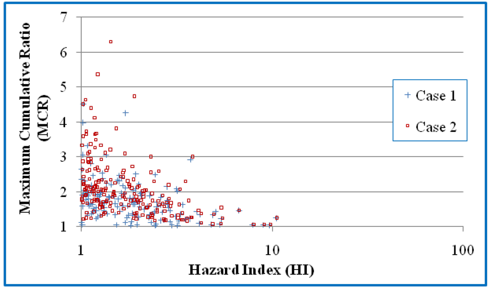
Figure 1.
A scatter plot of the HI and MCR values for the mixtures in the 618 mixtures. Case 1 assumes that NDs have a concentration of 0 and Case 2 assumes that NDs have concentrations of DL/20.5. Kendall correlation coefficients indicate a statistically significant negative correlation between MCR and HI for both cases (τ = −0.2132 and p < 0.0001 in Case 1; τ = −0.4362 and p < 0.0001 in Case 2).
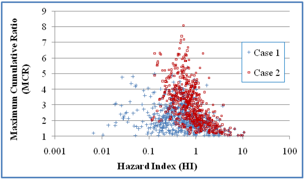
Figure 2.
A scatter plot of the HI and MCR values for the mixtures with HI values greater than 1. Case 1 assumes that NDs have a concentration of 0 and Case 2 assumes that NDs have concentrations of DL/20.5.
Figure 2.
A scatter plot of the HI and MCR values for the mixtures with HI values greater than 1. Case 1 assumes that NDs have a concentration of 0 and Case 2 assumes that NDs have concentrations of DL/20.5.
Table 6,
Table 7 and
Table 8 present the HI and MCR values for all mixtures, mixtures with HI greater and less than 1, and three subgroups of the mixtures respectively. Separate results are presented for Cases 1 and 2. Because of the contributions of the HQs associated with the NDs in Case 2, the HI values in Case 2 are always higher than those in Case 1 (0.19 higher on average for all mixtures). The MCR values in Case 2 are typically but not always higher than Case 1 (
Table 6).
Table 6.
HI and MCR values in the final dataset of 618 mixtures. Statistical significance was shown for the differences in HI and MCR values between Cases 1 and 2 (p < 0.0001, Wilcoxon test). Case 1 assumes that NDs have concentrations of 0 and Case 2 assumes that NDs have concentrations of DL/20.5.
| Cases | HI Values | MCR Values |
|---|
| Minimum | Maximum | Mean | Minimum | Maximum | Mean |
|---|
| Case 1 | 0.001 | 10.4 | 0.86 | 1.03 | 5.4 | 2.2 |
| Case 2 | 0.116 | 10.6 | 1.05 | 1.05 | 8.1 | 3.1 |
Dividing the 618 mixtures into two subgroups (those with HI less than 1 or HI greater than 1), shows that 158 (26%) and 208 (34%) of the mixtures have HI values greater than 1 in Cases 1 and 2, respectively. For both subgroups, the MCR values in Case 2 are higher than those in Case 1 but the mean difference is 1.3 for the mixtures with HI values less than 1 and 0.4 for mixtures with HI values greater than 1 (
Table 7).
Table 7.
Comparison of MCR values for mixtures with HI values greater or less than 1. For both groups of mixtures the MCR values in Case 2 are significantly higher than those in Case 1 (p < 0.0001 in Wilcoxon test). Case 1 assumes NDs have concentrations of 0 and Case 2 assumes that NDs have concentrations of DL/20.5. Min: Minimum; Max: Maximum.
| Cases | Mixtures with HI <1 | Mixtures with HI >1 |
|---|
| % of all mixtures | Min MCR | Max MCR | Mean MCR | % of all mixtures | Min MCR | Max MCR | Mean MCR |
|---|
| 1 | 74% | 1.03 | 5.4 | 2.3 | 26% | 1.0 | 4.5 | 1.7 |
| 2 | 66% | 1.16 | 8.1 | 3.6 | 34% | 1.1 | 6.3 | 2.1 |
MCR values in Cases 1 and 2 were also compared by choosing three portions of mixtures (49–51
st, 94–96
th, and 98–100
th centile ranges of the HI values of the mixtures). There are only small differences between Cases 1 and 2 in these groups and these differences had no statistical significance based on Wilcoxon test (
Table 8).
Table 8.
Comparison of the MCR values of three portions of mixtures in Cases 1 and 2. No statistical differences were found between the two cases for the three portions of samples in Wilcoxon test. The three portions of mixtures were chosen on the basis of HI (mixtures with HI values falling into 49–51st, 94–96th, and 98–100th centile ranges respectively). Case 1 assumes that NDs have concentrations of 0 and Case 2 assumes that NDs have concentrations of DL/20.5. Min: minimum; Max: maximum.
| Case | 49–51st Centile | 94–96th Centile | 98–100th Centile |
|---|
| Min MCR | Max MCR | Mean MCR | Min MCR | Max MCR | Mean MCR | Min MCR | Max MCR | Mean MCR |
|---|
| 1 | 1.86 | 4.0 | 2.8 | 1.2 | 2.1 | 1.6 | 1.04 | 1.5 | 1.2 |
| 2 | 1.52 | 3.3 | 2.6 | 1.2 | 2.2 | 1.5 | 1.05 | 1.5 | 1.2 |
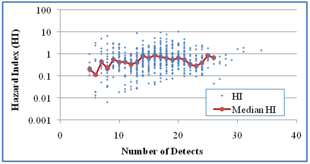
The relationship between HI and the number of detects in the mixtures was studied for Case 1 (
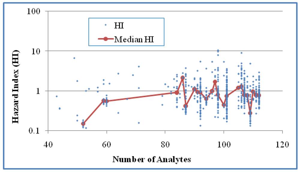
Figure 3). For Case 2 (
Figure 4), the number of analytes was used for examining this relationship since NDs were involved in the calculation of MCR values. For Case 1 there was a three-fold increase in HI when n was increased from 13 to 25, but no clear trend above an n of 25. The trend of increased HI values as n increased was statistically significant when based on HI values of individual mixtures (
p < 0.0001), but not when based on the medians of the HI values of grouped mixtures (
p > 0.05). No statistical significance was shown for this correlation in Case 2 either based on HI values of individual mixtures or median HI values of grouped mixtures for groups with at least five values (
p > 0.05). When grouping mixtures based on the same number of detects (
Figure 3) or analytes (
Figure 4), we obtained medians from groups of at least five values in order to generate more reliable medians for trend analysis. These observations suggest that an increase in the number of detected analytes is weakly associated with an increase in HI but an increase in the number of analytes is not associated with larger HI values.
Figure 3.
The relationship between HI and the number of detects in the samples for Case 1 (618 mixtures). A positive correlation was shown based on all mixtures (Kendall’s τ = 0.085 and p < 0.01) but not median HI of grouped mixtures for groups with at least five values (τ = 0.0913 and p > 0.05).
Figure 3.
The relationship between HI and the number of detects in the samples for Case 1 (618 mixtures). A positive correlation was shown based on all mixtures (Kendall’s τ = 0.085 and p < 0.01) but not median HI of grouped mixtures for groups with at least five values (τ = 0.0913 and p > 0.05).
Figure 4.
The relationship between HI and the number of analytes in the samples for Case 2 (618 mixtures). No statistical significance was shown for this correlation either based on all samples (Kendall’s τ = 0.0196 and p > 0.05) or median HI of grouped samples for groups with at least five values (τ = 0.0554 and p > 0.05).
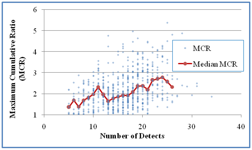
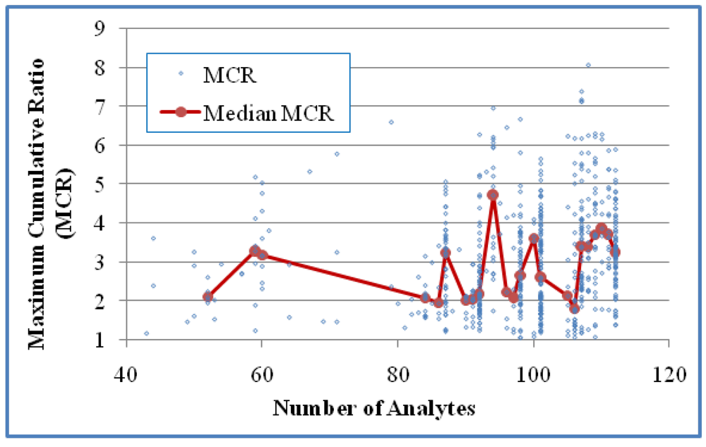
The relationship between MCR and n for the two cases are presented in
Figure 5 and
Figure 6. A positive correlation was shown for Case 1 either based on all mixtures (
p < 0.0001) or median MCR of grouped mixtures for groups with at least five values (
p < 0.001). A positive correlation for Case 2 was shown based on all mixtures (
p < 0.0001) and for median values of grouped mixtures (
p < 0.05). This suggests that increases in both the number of detects and the number of analytes are indicators of modest increases in MCR values. The MCR values for mixtures measured in samples with 5–10 detects ranged from 1.0 to 2.0 while the MCR values for mixtures measured in samples with 15–25 detects had a wider range (1.0 to 5.0).
Figure 5.
The relationship between MCR and the number of detects in the samples for Case 1 (618 mixtures). A positive correlation was shown either based on all mixtures (Kendall’s τ = 0.2511 and p < 0.0001) or median MCR of grouped mixtures for groups with at least five values (τ = 0.6826 and p < 0.0001).
Figure 6.
The relationship between MCR and the number of analytes in the samples for Case 2 (618 mixtures). A positive correlation was shown based either on all mixtures (Kendall’s τ = 0.1501 and p < 0.0001) or on median MCR values of grouped mixtures for groups with at least five values (τ = 0.3202 and p < 0.05).
3.5. Discussion
The issue of cumulative exposures to chemicals has been drawing increasing attention in the fields of toxicology and risk assessment. The MCR is a tool that can help evaluate the need forCRAs. Smaller MCR values indicate that a single chemical is driving the total toxicity resulting from cumulative exposures.
Price and Han [
1] previously investigated the range of HI and MCR values for a group of PPPs measured in surface water samples. In this paper, we have performed a similar analysis on a second dataset of organic and inorganic compounds in ground water wells used as drinking water supplies across the U.S. [
3]. These samples differ in terms of source (ground water
versus surface water), HI values (mean HI value of 0.87
versus 0.14 when setting NDs at 0), and the number and variety of analytes (a range of organic and inorganic compounds
versus PPPs). The PPPs in the surface water samples resulted mainly from agricultural use of PPPs while the compounds in this study came from natural sources, uncontrolled waste disposal, as well as PPP use. The top six contributors to the HI values of mixtures are inorganic chemicals (
Table 5) which may occur naturally or could result from human activity.
Despite these differences, many of the findings in the first study are also observed in this dataset. The vast majority of mixtures in the ground water samples have MCR values below 5 (
Figure 1) with an average MCR value of 2.2–3.1 (
Table 6). These findings suggest that the HI values of most mixtures are dominated by just a few chemicals.
Figure 1 and
Figure 2 indicate that, as an overall trend, MCR values decrease as HI values increase. This trend is more obvious when only focusing on the mixtures with HI values greater than one. The trends suggest that mixtures with higher toxicity are in general dominated by the toxicity of the primary chemical and have less need for a CRA.
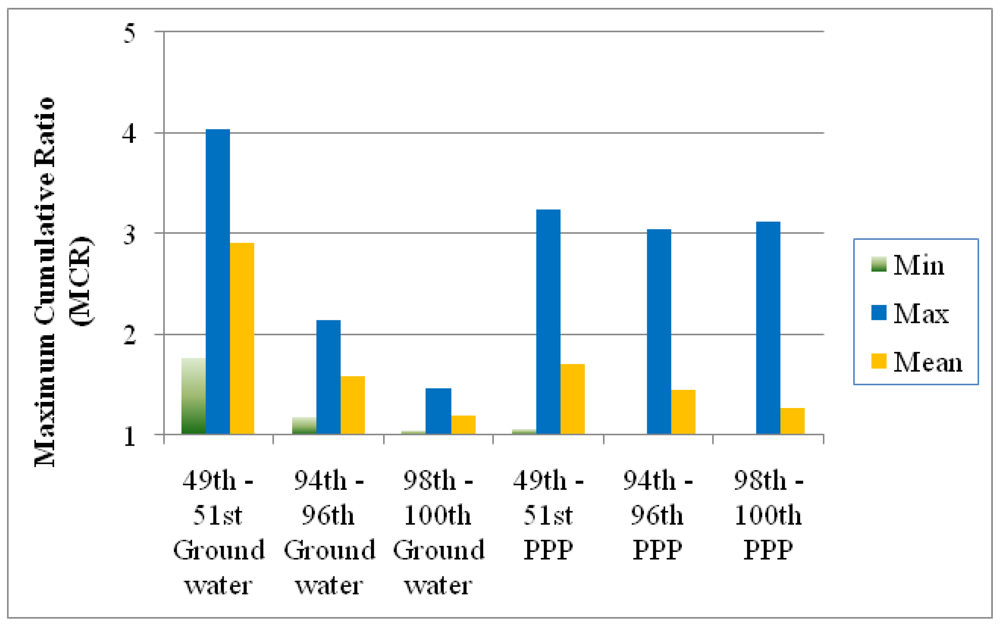
Figure 7.
Comparison of the MCR values in three groups of the mixtures in the surface water samples analyzed for PPPs [
1] and the results from this study (ground water samples). The three groups of mixtures were chosen on the basis of HI (mixtures with HI values falling into 49–51
st, 94–96
th, and 98–100
th centile ranges respectively). Min: minimum; Max: maximum.
Figure 7 presents the minimums, maximums, and means of MCR in mixtures with HI values falling in the 49–51
st, 94–96
th and 98–100
th centile ranges of HI values. The data were taken from our original publication [
1] and the new work presented here. The MCR values are higher for the mixtures with typical HI values. This may be a reflection of the fact that more compounds and more detects occurred in groundwater study. MCR values in the ground water study clearly decrease with increasing toxicity for both datasets. The average MCR values, as presented in yellow, are higher in mixtures with HI values near the median and 95
th centiles but smaller for mixtures with HI values in the top two centiles. In this dataset the maximum MCR values in the three groups also declined suggesting a stronger trend than that observed in the surface water data.


