Time-series MODIS Image-based Retrieval and Distribution Analysis of Total Suspended Matter Concentrations in Lake Taihu (China)

Abstract
:1. Introduction
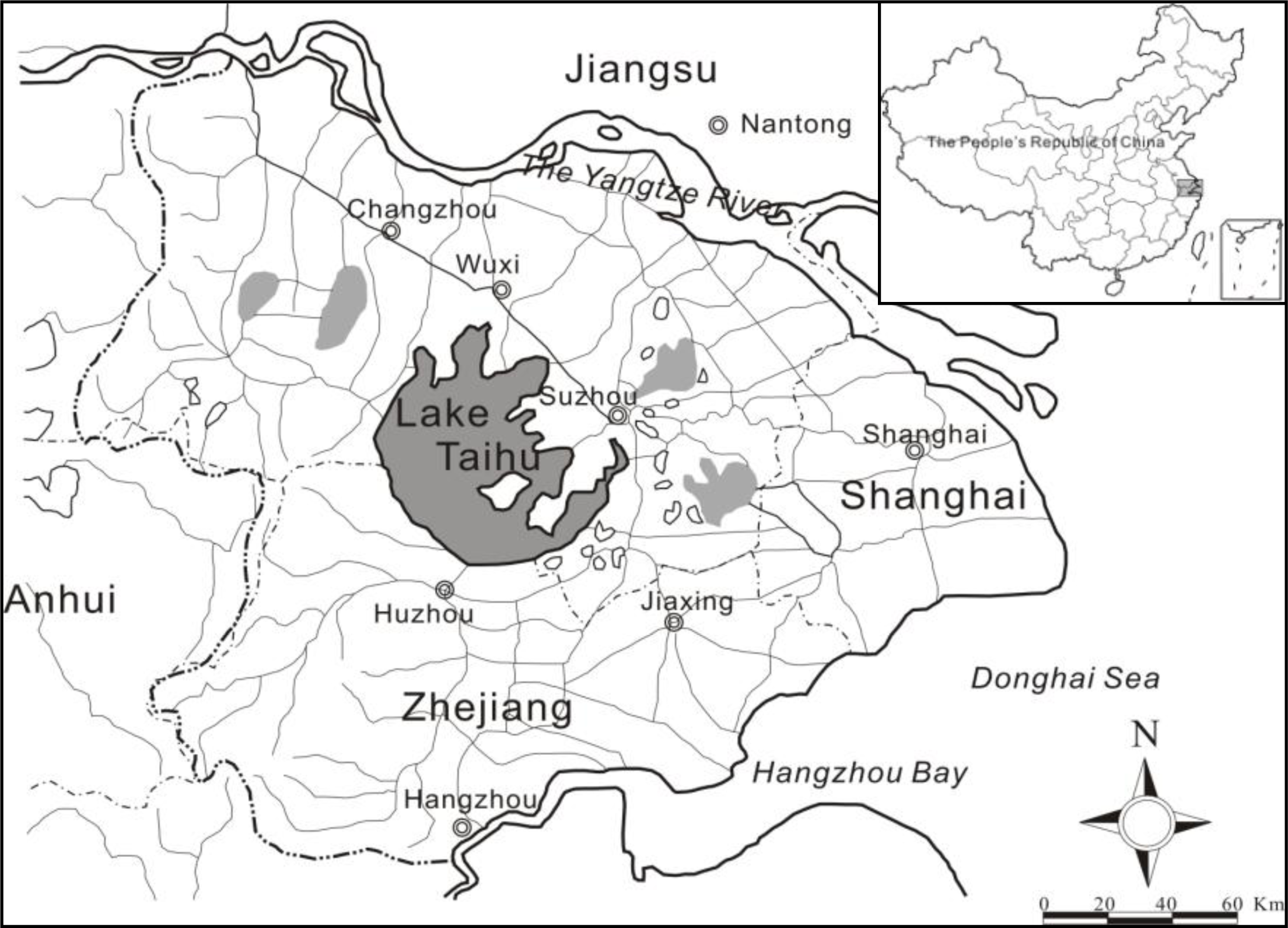
2. Study Area
3. Methods
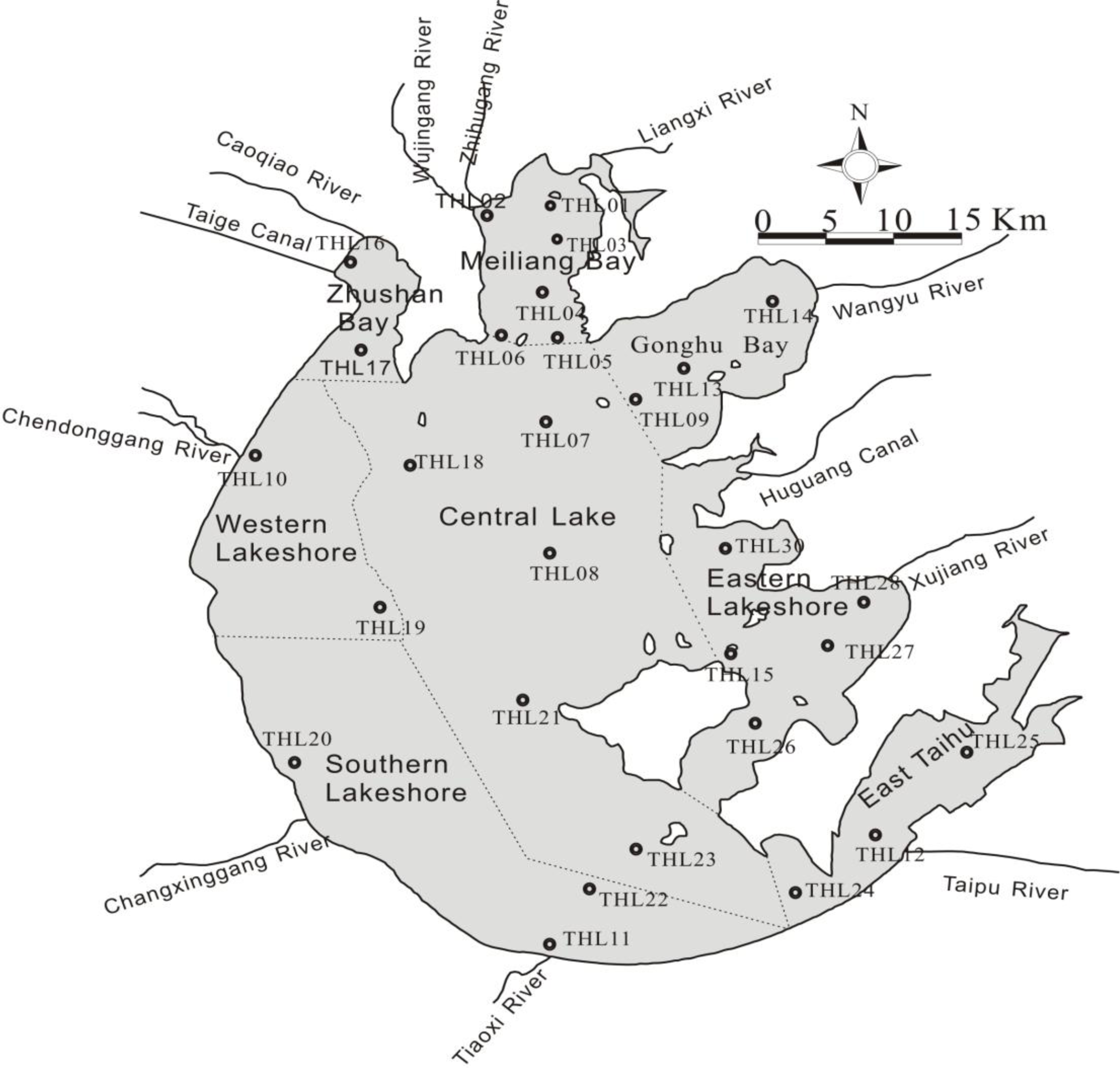
3.1. Field Survey
3.2. MODIS Imagery
3.3. Retrieval of Total Suspended Matter Concentrations from MODIS Data
4. Results
5. Discussion
5.1. MODIS Bands Retrieving TSM
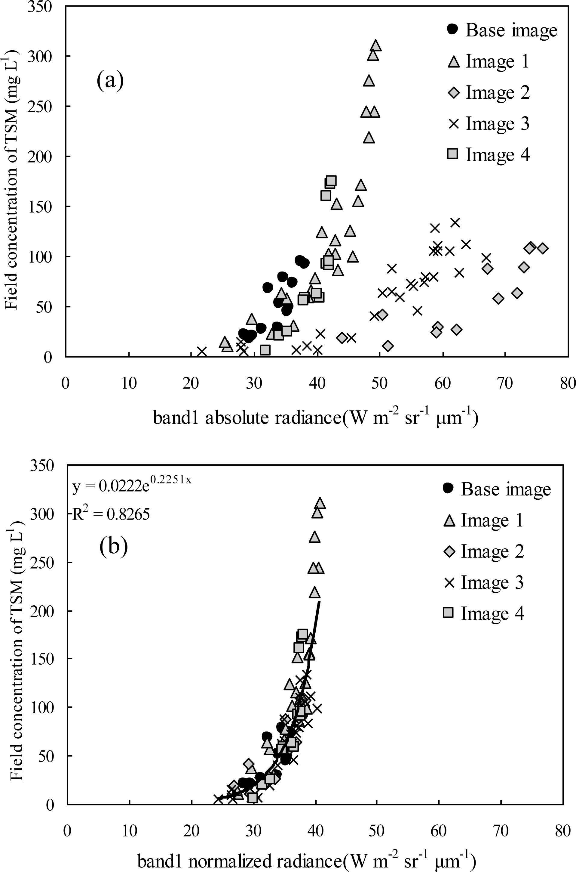
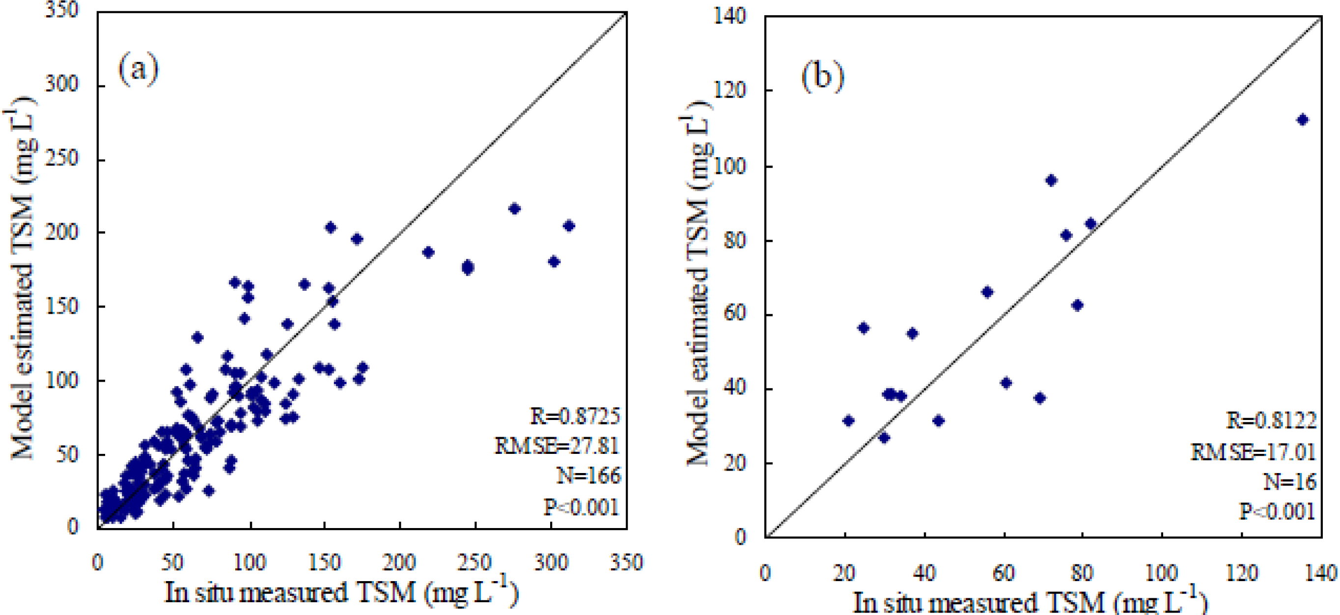
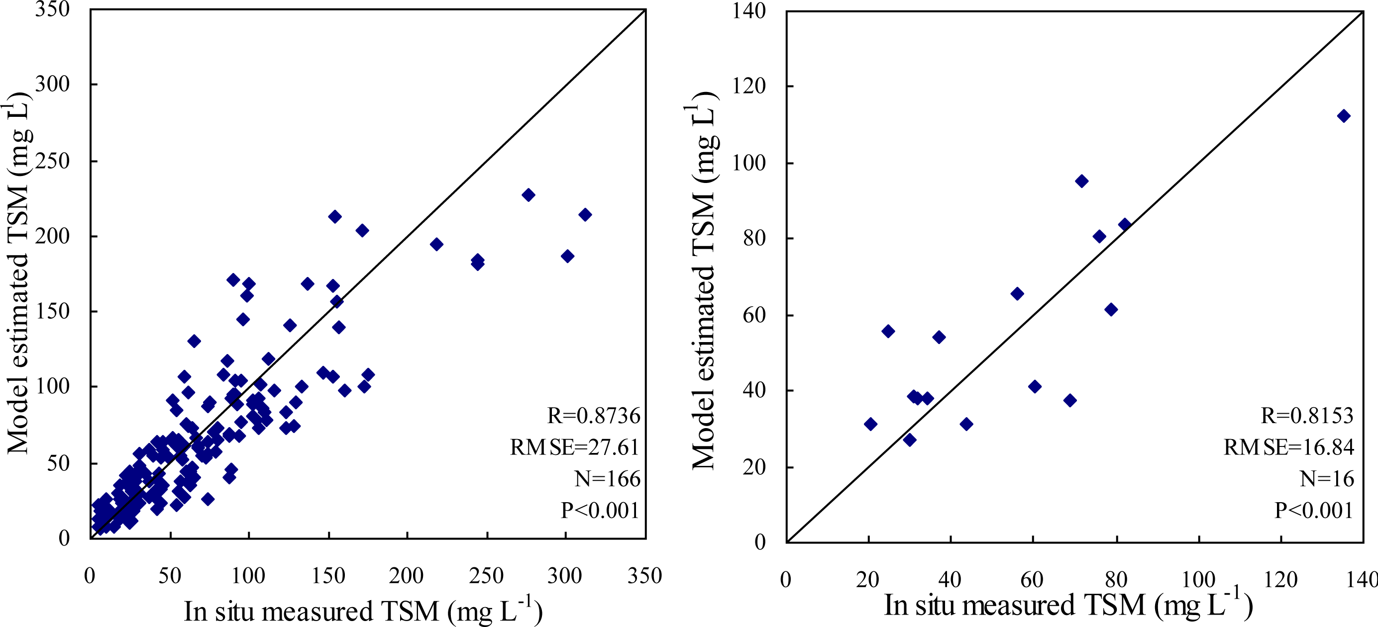
5.2. Model Performance Analysis
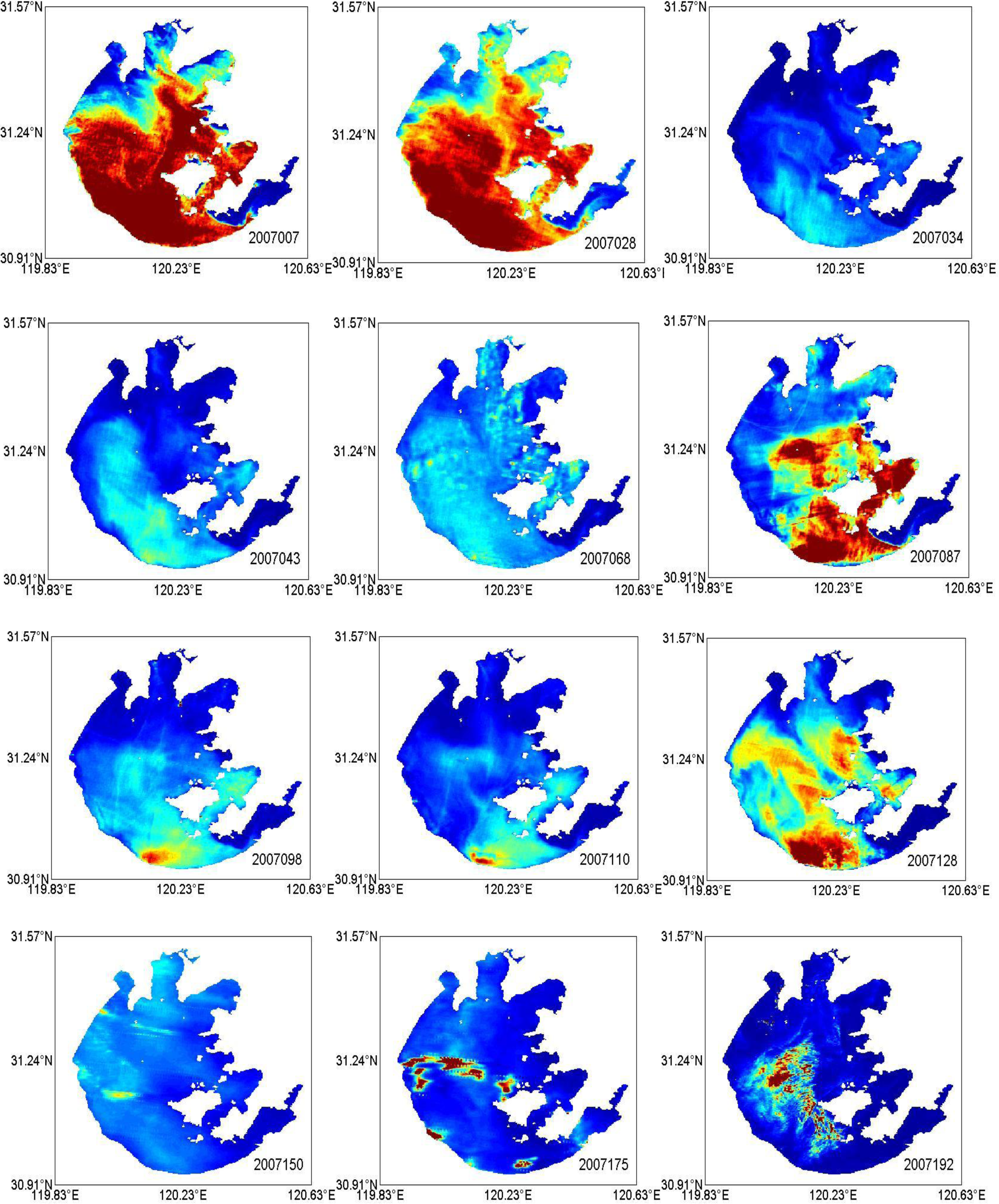
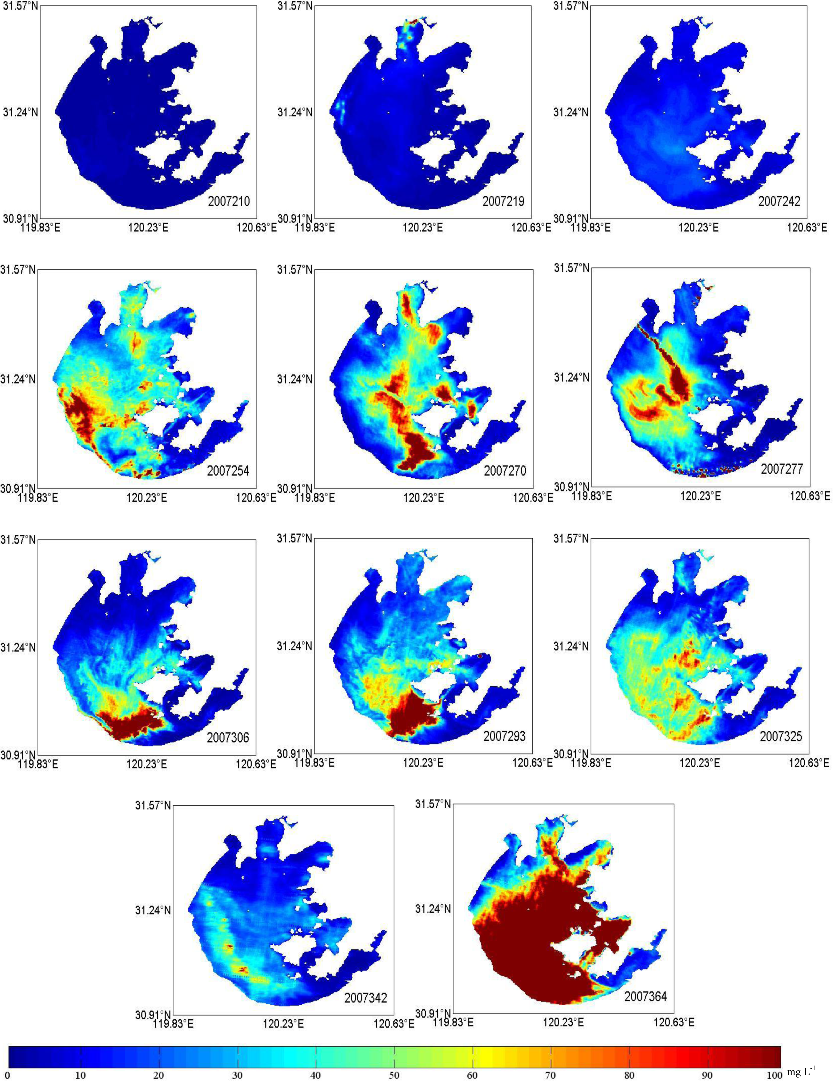
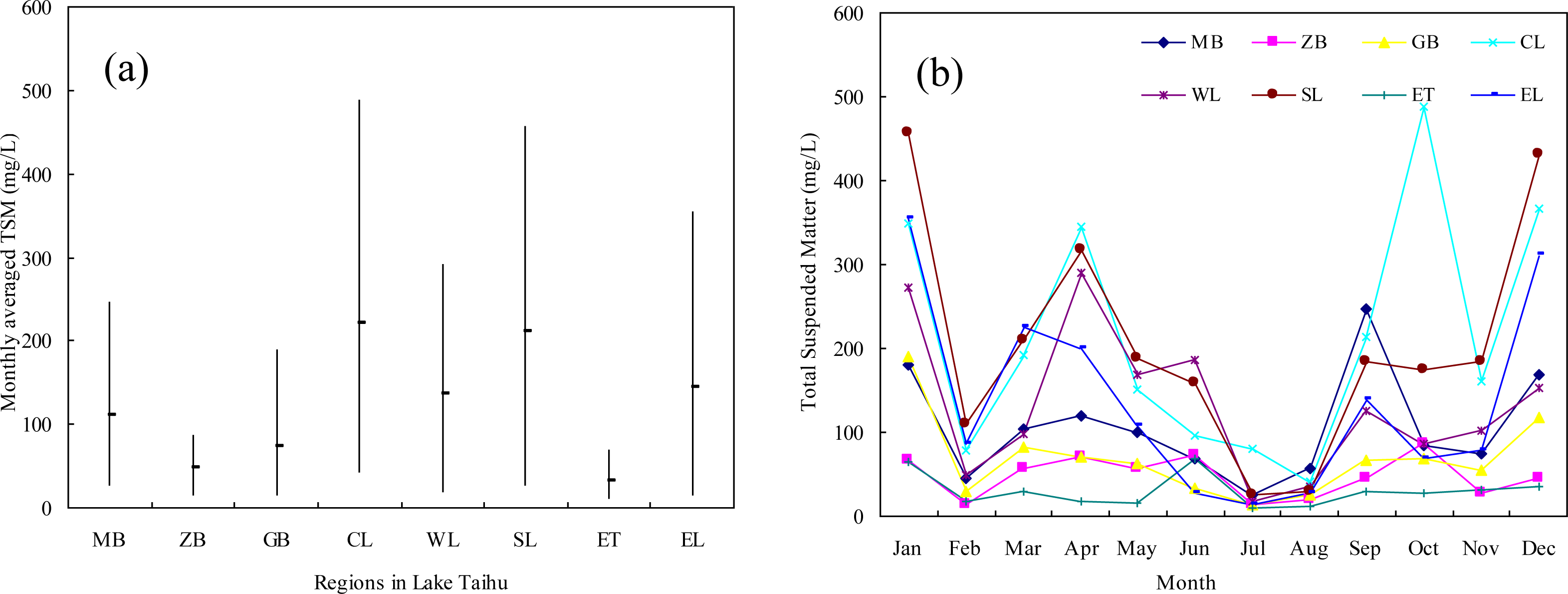
5.3. Distribution of TSM in Lake Taihu in 2007
6. Conclusions
Acknowledgments
References and Notes
- Onderka, M; Pekarova, P. Retrieval of suspended particulate matter concentrations in the Danube River from Landsat ETM data. Sci. Total Environ 2008, 397, 238–243. [Google Scholar]
- Kritikos, H; Yorinks, L; Smith, H. Suspended solids analysis using ERTSA data. Remote Sens. Environ 1974, 3, 69–80. [Google Scholar]
- Sterckx, S; Knaeps, E; Bollen, M; Trouw, K; Houthuys, R. Retrieval of suspended sediment from advanced hyperspectral sensor data in the Scheldt estuary at different stages in the tidal cycle. Marine Geodesy 2007, 30, 97–108. [Google Scholar]
- Sipelgas, L; Raudsepp, U; Kouts, T. Operational monitoring of suspended matter distribution using MODIS images and numerical modeling. Adv. Space Res 2006, 38, 2182–2188. [Google Scholar]
- Wang, YP; Xia, H; Fu, JM; Sheng, GY. Water quality change in reservoirs of Shenzhen, China: detection using LANDSAT/TM data. Sci. Total Environ 2004, 328, 195–206. [Google Scholar]
- Pozdnyakov, D; Shuchman, R; Korosov, A; Hatt, C. Operational algorithm for the retrieval of water quality in the Great Lakes. Remote Sens. Environ 2005, 97, 352–370. [Google Scholar]
- D'Sa, EJ; Miller, RL; McKee, BA. Suspended particulate matter dynamics in coastal waters from ocean color: Application to the northern Gulf of Mexico. Geophys. Res. Lett 2007, 34, 1–6. [Google Scholar]
- Ma, RH; Tang, JW; Dai, JF. Bio-optical model with optimal parameter suitable for Taihu Lake in water colour remote sensing. Int. J. Remote Sens 2006, 27, 4305–4328. [Google Scholar]
- Zhang, B; Li, J; Shen, Q; Chen, D. A bio-optical model based method of estimating total suspended matter of Lake Taihu from near-infrared remote sensing reflectance. Environ. Monit. Assess 2008, 145, 339–347. [Google Scholar]
- Ma, RH; Song, QJ; Tang, JW; Pan, DL. A simple empirical model for remote sensing reflectance of Lake Taihu waters in autumn. J. Lake Sci 2007, 19, 227–234. [Google Scholar]
- Wang, SX; Jiao, YQ; Zhou, Y; Wang, LT. Determination of Suspended sediment concentration of Taihu Lake based on season difference using multi-temporal MODIS image data. IEEE International Geoscience and Remote Sensing Symposium, Barcelona, SPAIN, July 2007; pp. 4570–4573.
- Guang, J; Wei, YC; Huang, JZ; Li, YM; Wen, JG; Guo, JP. Seasonal suspended sediment estimating models in Lake Taihu using remote sensing data. J. Lake Sci 2007, 19, 241–249. [Google Scholar]
- Ma, RH; Dai, JF. Investigation of chlorophyll-a and total suspended matter concentrations using Landsat ETM and field spectral measurement in Taihu Lake, China. Int. J. Remote Sens 2005, 26, 2779–2795. [Google Scholar]
- Hu, CM; Chen, ZQ; Clayton, TD; Swarzenski, P; Brock, JC; Muller-Karger, FE. Assessment of estuarine water-quality indicators using MODIS medium-resolution bands: Initial results from Tampa Bay, FL. Remote Sens. Environ 2004, 93, 423–441. [Google Scholar]
- Schott, JR; Salvaggio, C; Volchok, WJ. Radiometric scene normalization using pseudo invariant features. Remote Sens. Environ 1988, 26, 1–14. [Google Scholar]
- Elvidge, CD; Yuan, D; Weerackoon, RD; Lunetta, RS. Relative radiometric normalization of Landsat Multispectral Scanner (MSS) data using an automatic scattergram-controlled regression. Photogramm Eng. Rem. S 1995, 61, 1255–1260. [Google Scholar]
- Coppin, P; Jonckheere, I; Nackaerts, K; Muys, B; Lambin, E. Digital change detection methods in ecosystem monitoring: a review. Int. J. Remote Sens 2004, 25, 1565–1596. [Google Scholar]
- Vicente-Serrano, SM; Perez-Cabello, F; Lasanta, T. Assessment of radiometric correction techniques in analyzing vegetation variability and change using time series of Landsat images. Remote Sens. Environ 2008, 112, 3916–3934. [Google Scholar]
- Hall, FG; Strebel, DE; Nickeson, JE; Goetz, SJ. Radiometric rectification Toward a common radiometric response among multidate, multisensor images. Remote Sens. Environ 1991, 35, 11–27. [Google Scholar]
- Song, C; Woodcock, CE; Seto, KC; Lenney, MP; Macomber, SA. Classification and change detection using Landsat TM data: When and how to correct atmospheric effects? Remote Sens. Environ 2001, 75, 230–244. [Google Scholar]
- Janzen, DT; Fredeen, AL; Wheate, RD. Radiometric correction techniques and accuracy assessment for Landsat TM data in remote forested regions. Can. J. Remote Sens 2006, 32, 330–340. [Google Scholar]
- Schroeder, TA; Cohen, WB; Song, CH; Canty, MJ; Yang, ZQ. Radiometric correction of multi-temporal Landsat data for characterization of early successional forest patterns in western Oregon. Remote Sens. Environ 2006, 103, 16–26. [Google Scholar]
- Du, Y; Teillet, PM; Cihlar, J. Radiometric normalization of multitemporal high-resolution satellite images with quality control for land cover change detection. Remote Sens. Environ 2002, 82, 123–134. [Google Scholar]
- Chen, XX; Vierling, L; Deering, D. A simple and effective radiometric correction method to improve landscape change detection across sensors and across time. Remote Sens. Environ 2005, 98, 63–79. [Google Scholar]
- Miller, RL; McKee, BA. Using MODIS Terra 250 m imagery to map concentrations of total suspended matter in coastal waters. Remote Sens. Environ 2004, 93, 259–266. [Google Scholar]
- Hu, CM; Chen, ZQ; Clayton, TD; Swarzenski, P; Brock, JC; Muller-Karger, FE. Assessment of estuarine water-quality indicators using MODIS medium-resolution bands: Initial results from Tampa Bay, FL. Remote Sens. Environ 2004, 93, 423–441. [Google Scholar]
- Chen, ZQ; Hu, CM; Muller-Karger, F. Monitoring turbidity in Tampa Bay using MODIS/Aqua 250-m imagery. Remote Sens. Environ 2007, 109, 207–220. [Google Scholar]
- Gin, KYH; Koh, ST; Lin, II; Chan, ES. Application of spectral signatures and color ratio to estimate chlorophyll in Singapore’s coastal water. Estuar. Coast. Shelf S 2002, 55, 719–728. [Google Scholar]
- Lu, H; Wei, XH. Quantitative retrieval of solid suspended matter concentration using MODIS 250m band. Geo-inform. Sci 2008, 10, 151–155. [Google Scholar]
- Zhang, YL; Qin, BQ; Chen, WM; Luo, LC. A study on total suspended matter in Lake Taihu. Resour. Environ. Yangtze Basin 2004, 13, 266–271. [Google Scholar]
- Zhang, YL; Qian, BQ; Chen, WM; Hu, WP; Yang, DT. Distribution, seasonal variation and correlation analysis of the transparency in Taihu Lake. T. Oceanol. Limnol 2003, 2, 30–35. [Google Scholar]
- Luo, LC; Qin, BQ. Comparison between wave effects and current effects on sediment resuspension in Lake Taihu. Hydrol 2003, 23, 1–4. [Google Scholar]
- Pang, Y; Li, YP; Luo, LC. Simulation on transparency in Taihu Lake. Sci. China Ser. D 2005, 35, 145–156. [Google Scholar]
- Le, CF; Li, YM; Zhang, YL; Sun, DY; Wu, L. Water color parameter spatial distribution character and influence on hygrophyte photosynthesis in Taihu Lake. Chinese J. Appl. Ecol 2007, 18, 2491–2496. [Google Scholar]
- Shi, K; Li, YM; Lv, H; Sun, DY; Huang, CC; Wang, YF; Jin, X. Depth profile of suspended particle scattering coefficient and its impact factors in Taihu Lake. Environ. Sci 2010, 31, 598–605. [Google Scholar]


| Date of observations | Number of samples | Concentration scope of TSM (mg L−1) | Date of MODIS image |
|---|---|---|---|
| Jan 17 | 13 | 17.74–94.36 | Jan 17 |
| Feb 20 to 22 | 28 | 11.35–311.40 | Feb 20 |
| Apr 15 | 13 | 10.40–146.08 | Apr 15 |
| May 19 to 20 | 13 | 10.96–108.30 | May 22 |
| Jul 14 | 13 | 4.32–88.68 | Jul 16 |
| Aug 18 | 28 | 5.23–133.40 | Aug 15 |
| Sep 14 to 15 | 13 | 18.92–128.80 | Sep 16 |
| Oct 13 to 14 | 11 | 24.60–63.16 | Oct 11 |
| Nov 18 | 21 | 6.54–153.95 | Nov 21 |
| Dec 14 to 16 | 13 | 5.48–174.60 | Dec 14 |
| Retrieval Models | R | s.e. | F |
|---|---|---|---|
| Ln(TSM)= 0.015 × b1 + 0.003 ×b12 −0.282 | 0.8712 | 0.439 | 256.310 |
| 0.7906 | 0.546 | 272.919 | |
| 0.8725 | 0.417 | 292.994 | |
| 0.8736 | 0.418 | 291.665 |
© 2010 by the authors; licensee Molecular Diversity Preservation International, Basel, Switzerland. This article is an open-access article distributed under the terms and conditions of the Creative Commons Attribution license (http://creativecommons.org/licenses/by/3.0/).
Share and Cite
Zhang, Y.; Lin, S.; Liu, J.; Qian, X.; Ge, Y. Time-series MODIS Image-based Retrieval and Distribution Analysis of Total Suspended Matter Concentrations in Lake Taihu (China). Int. J. Environ. Res. Public Health 2010, 7, 3545-3560. https://doi.org/10.3390/ijerph7093545
Zhang Y, Lin S, Liu J, Qian X, Ge Y. Time-series MODIS Image-based Retrieval and Distribution Analysis of Total Suspended Matter Concentrations in Lake Taihu (China). International Journal of Environmental Research and Public Health. 2010; 7(9):3545-3560. https://doi.org/10.3390/ijerph7093545
Chicago/Turabian StyleZhang, Yuchao, Shan Lin, Jianping Liu, Xin Qian, and Yi Ge. 2010. "Time-series MODIS Image-based Retrieval and Distribution Analysis of Total Suspended Matter Concentrations in Lake Taihu (China)" International Journal of Environmental Research and Public Health 7, no. 9: 3545-3560. https://doi.org/10.3390/ijerph7093545