1. Introduction
Count data models have been widely used to estimate the predictors of health care demand [
1–
7]. Most analyses use household surveys collecting information about health care provider types and number of visits made to different types of providers during the recall period. An important issue to be considered in estimating the effects of health insurance on the demand for health care in these settings is therefore to establish whether the demand variable is generated as a discrete and mutually exclusive choice (e.g., types of providers visited in the event of an illness) or is in the form of a count or rate (e.g., number of visits made to a particular provider). The latter is usually modeled using count data models and their variants [
8].
In estimating health care demand, complexities arise because the underlying behaviors driving health care utilization may have implications for the choice of the most appropriate model [
7]. Further, as people demand both health insurance and health care depending on their health status, whether the model suffers from bias (due to endogeneity of the choice of insurance status and demand) should be scrutinized [
9,
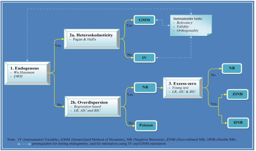
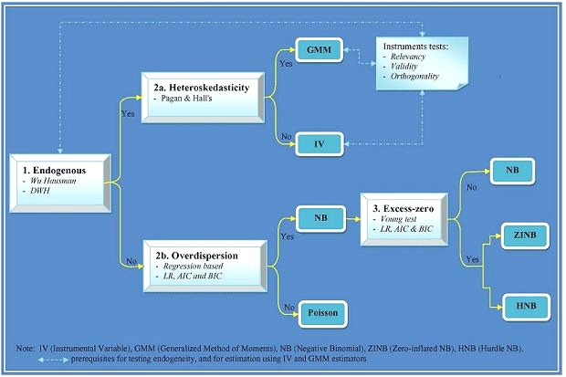
10]. Deciding on a particular model appropriate for estimating health care demand is a difficult process that is often poorly documented in the health economics literature. The purpose of this paper is to document the complete process by which we developed guidelines for the selection of an appropriate count data model for health insurance and health care demand and to choose a particular count data model in estimating the number of outpatient visits.
In practice we will estimate the relationship between health insurance and the number of outpatient visits to public and private health care providers in Indonesia. There are previously published studies on health insurance and health care demand [
9–
11]; Indonesia deserves special attention as it is a developing country committed to universal coverage through a national health insurance program (NHIP). This article provides evidence on whether such a policy would be welfare-enhancing in terms of increasing access to formal health care in Indonesia.
This study also confronts directly the statistical tradeoffs associated with correcting for endogenous regressors (
i.e., correcting for endogeneity when it is absent results in larger standard errors, loss of precision [
10], and efficiency [
12]). We explore two classes of count data models. The first class is characterized by a primary equation with a discrete dependent variable. This class includes standard count data models such as restricted Poisson, negative binomial zero-inflated, and hurdle models. The second class extends the features of the first class to accommodate endogenous regressors, including instrumental variables [
12,
13] and generalized method of moments [
14] techniques.
2. Health Insurance Context and Potential Source of Endogeneity
Table 1 provides summary characteristics of health insurance schemes. The Indonesian government has mandated health insurance for civil servants (
Askes) since 1968. This scheme covers all civil servants, civil servant and armed forces pensioners, and their families and survivors. Civil servants and pensioners are automatically enrolled in this scheme. Eligible dependents include spouse and the first two children, with the cut-off age for dependent children depending on education status. The contribution is 4 percent of basic salary shared equally by employees and the government as employer. The scheme, managed by a state-owned company (
PT Askes), covers about 14 million beneficiaries. Since
Askes is compulsory, people may choose civil service employment based on their health status. Therefore, endogeneity of insurance status and health care demand may arise for those with less favourable health status who choose civil service employment with compulsory health care insurance benefits. Similarly, healthier workers may be more likely to choose self-employment or smaller private firms to avoid mandatory health insurance premiums.
In 1992, the government passed a Social Security Act (SSA) mandating enrolment of private employees in either privately-provided insurance schemes or the government-provided
Jamsostek insurance scheme (which includes provident funds, death benefits, and worker’s compensation in addition to health benefits). SSA regulations stipulate that private employers with total salary costs of more than 1 million
Rupiah per month (roughly $100 at current exchange rates) are required to enroll their employees and dependents in qualified health insurance plans managed by
PT Jamsostek. However, the health benefit as required by the SSA is compulsory but optional, that is employers who have a better scheme than the one covered by
Jamsostek may opt out to this scheme. This policy makes this scheme covers only 3 million workers out of about approximately 100 million workers who are eligible [
15].
Jamsostek covers spouses and up to three dependent children less than 21 years of age with benefits include outpatient and inpatient care at both public and public health care providers. Premiums, which are capped at 3percent of basic salary for unmarried and 6percent for married employees, are paid solely by employers so
Jamsostek is non-contributory. This policy may lead employers to choose
Jamsostek for their low income employees with health problems while healthier employees with higher incomes will opt out. Thus, it is likely that endogeneity is an issue for
Jamsostek membership as well.
The government also enacted the Insurance Act in 1992 which allows private insurance firms to sell health insurance products. These schemes usually offer both public and private health providers in their provider networks. The consensus estimate of the number of people with private health insurance is 5 million [
15]. The health insurance literature has documented selection bias in private insurance demand; therefore one should suspect endogeneity of insurance status while estimating health care demand given private insurance [
10].
Even given public policy and this menu of insurance opportunities, in 2004 only a small fraction of the Indonesian population (<15 percent) was covered by any health insurance. Motivated largely by the expectation that health insurance improves access to health care, the president signed a National Social Security Law in 2004 which will used as a basis for introducing an NHIP in the country.
4. Data and Variables
The data for this study come from the second round of the Indonesian Family Life Survey (IFLS2) carried out by the RAND Corporation. The first round of survey (IFLS1) included interviews with 22,347 individuals from 7,224 households. The IFLS2 re-contacted the same households and succeeded in re-interviewing 93.5percent of IFLS1 households (6751 households with over 33,000 individuals). An overview of the survey is described in [
25] for IFLS1 and [
26] for IFLS2.
This study considers two mutually exclusive measures of OP visits: public and private providers. Not all insurance schemes offer health care services from both public and private providers and sample distributions of these variables (presented in
Table 2) show that approximately 85 percent of IFLS individuals had zero visits to public OP and about 92 percent had zero private OP visits. The sample means for the number of visits to public and private OP were 0.28 and 0.15 respectively while the sample variances were 0.67 and 0.43 respectively. The ratio between the sample variance and the sample mean for the number to public and private OP visits were 2.39 and 2.87, respectively. These averages indicate the observed data is over-dispersed.
Two insurance variables,
Askes and
Private, enter demand
Equation (1) as dummy variables.
Askes represents mandatory insurance for civil servants and entitles beneficiaries to comprehensive health care from public providers only.
Private represents both
Jamsostek (insurance for private employees) and private insurance schemes and therefore may be entitling beneficiaries to care from both public and private providers. Since the effects of health insurance on health care demand might differ across income groups, an interaction term for insurance and income was included in the demand model. This interaction allows one to test whether income has different effects of insurance on the number of outpatient visits.
In demand
Equation (1), the health-status vector consisted of dummy variables indicating the presence of symptoms, self-assessed general health (GHS) and severity of illness. A score assessing physical ability in the performance of daily activities (ADLs) was also included (with higher scores indicating worse ability). The vector of demographic variables consisted of age (years), gender (1/0), marital status (1/0), dummies for education, income (log natural), electricity usage (1/0), and the natural log of one-way travel time and travel cost to health facilities. To control for regional differences we used dummy variables for urban and seven regions (rural and Jakarta serving as the reference groups). Summary statistics for the variables used in the demand
Equation (1) are presented in
Table 3.
The endogeneity test as well as IV and GMM estimators can only be applied if one finds appropriate instruments. We propose candidate instrumental variables z that may satisfy two requirements [
14]: they should be correlated with the endogenous variable(s) and they should be orthogonal to the error process. The proposed z are presented in
Appendix A.
We estimated reduced form regressions of the endogenous variables on the full set of instruments (
Equation (2)) using a probit model. The main objective was to generate the predicted values of insurance to be included as an additional instrument in IV and GMM techniques. The basic conclusion was that the insurance decision was more determined by income, education, age and location variables. All the proposed instruments in
Appendix A except household head’s employment type had a positive correlation with choice of
Askes insurance (
p-value < 0.01). For
Private insurance, only four of the proposed instruments (household head’s employment type, spouse, if active in community meetings and if housing occupied) had significant positive correlations.
R2 reveals that the covariates in the
Askes insurance estimates explained 30 percent of the overall variation, but only 20 percent of
Private insurance variation. The joint Wald statistics shows all covariates were jointly significant in either insurance equation at the one percent level. After trying different specifications, we have selected from the proposed
z two different subsets as final instruments for the
Askes and
Private equations (see
Appendix A). These subsets of
z were included in the estimation of insurance model (
Equation (2)) but excluded from the demand model (
Equation (1)).
6. Discussion
This study has estimated the relationship between health insurance and the number of public and private outpatient visits in Indonesia. We have explored two econometric classes of count data models: a specification that ignores endogeneity of insurance choice and a specification that considers endogeneity of insurance choice. Although both IV and GMM estimators allow for controlling endogeneity of the insurance in the estimation [
13,
14], they are generally less efficient than the ML estimation of standard count data [
12]. Hence, there was a trade-off between loss of precision and having biased parameter estimates [
10]. Since arriving at the choice of most appropriate econometric technique is often a difficult process but not often documented in the literature in great detail, in this paper we have described criteria that helped us select most appropriate econometric technique.
We observed evidence for endogeneity (of insurance status) in the number of public OP visits. This led us to conclude that the GMM estimator is the best to model the number of public outpatient visits. Comparison of estimation results obtained from all econometric techniques explored in the study (complete results available upon request) reveals that the parameter estimates for the
Askes insurance after controlling for endogeneity were higher than without controlling for it. This suggests that estimates of demand given insurance might depend on the empirical econometric specification used in the analysis. If the final model is not chosen based on stringent criteria as applied in this case, the calculation of premiums and prediction of financial sustainability of an insurance scheme might be underestimated. Our findings confirm empirical studies done in Ecuador and Ireland. Waters [
10] found that after controlling for endogeneity of insurance, the beneficiaries of general health insurance programmes in Ecuador significantly increased their demand for curative health care by about 30 percent, whilst not controlling for endogeneity of insurance the demand effect was only 11 percent. In Ireland, Harmon and Nolan [
28] found that treating insurance as exogenous, the probability of having a hospital stay was 3 percent higher for those with health insurance. When insurance was treated endogenously, the effects approximately double (6 percent).
In the case of private visits, several statistical tests suggested that the HNB hurdle specification is superior to the standard one-part specification. The use of HNB is justified by the fact that health care use in this study is measured by number of contacts instead of the total cost of all contacts [
7]. Our finding is line with previous studies [
3], and confirms the importance of distinguishing between factors that affect the propensity for contacting health care providers and factors that determine the volume of utilization once contact has been made [
16]. Bogu [
29] also suggests that count data models most commonly used are the hurdle model and the finite mixture negative binomial. The validity of hurdle specification is suspect if individuals have multiple illness episodes or multiple first contacts or the first contact belongs to an illness episode of the preceding illness [
3,
14,
16]. Since utilization data in this study is derived from a 4-week recall period, both multiple illness episodes and multiple first contacts seem unlikely here. In addition, this study included several measures of current health conditions and an ADL score reflecting long-term health status. As they were not significant in the second stage of the HNB model, the HNB retains its superiority over other candidate models.
The HNB estimates confirm that
Askes insurance exhibited a negative relationship in both contact and frequency decisions for private OP which is consistent with
a priori expectations as the scheme entitles beneficiaries to services at public providers only. For
Private insurance, the coefficients show positive relationships in both decision stages but are significant only in the contact decision. The motivation of the hurdle model comes from ‘principal-agent’ theories of the demand for health care [
4]. In this regard, however, our results do not support the possibility of supplier-induced demand due to insurance. This might be the result of a strict utilization review program managed by the insurer. In addition, our results show that the main determinants of the frequency decision are need-based. This is consistent with previous studies that found no evidence of such behavior [
3].
Another way to look into the evidence of supply induced demand (SID) for health care is to examine how the doctors’ density affects demand. Physician density in Indonesia is higher in urban areas. Physicians practicing in urban areas facing negative income shocks could use their dual role—both as evaluator and supplier—to induce demand [
30]. In our models, the urban dummy turned out to be positive and significant in both decisions for visits to private OP, suggesting there is evidence SID where private provider competition is likely. However, future research is needed to validate our finding by including a variable that measures physician density directly.
The finding that insurance increases individuals’ propensity for health care utilization is important for policy makers, particularly in Indonesia where current debate is dominated by discussions regarding improving access to care and the introduction of national health insurance scheme. Although such findings have been reported elsewhere [
9–
11,
28], our results are specific to two different types insurance (
Askes with public providers only and
Private with both public and private providers). The large effect observed in the use of private providers compared with public ones by
Private insurance beneficiaries may be explained in the light of perceived quality of care. Theoretically, insurance reduces the effective price that beneficiaries pay for health care [
30]. Insured people, given provider networks, choose the alternative that yields the highest satisfaction (utility). As this would mean increasing perceived quality and decreasing prices, the ultimate choice of provider actually reflects the relative trade-off between price and quality that individuals prefer. By offering private providers (perceived to have better quality),
Private insurance reduces the relative price of quality, and hence the beneficiaries were more likely to use private providers. If there is a quality effect, our findings would imply that public providers may need strategies that would change people’s perceptions about their quality of care.
Another finding from this analysis bears more discussion. A negative (and statistically significant) relationship to health care demand of Private insurance/income interaction in the HNB estimates indicates the effects of Private insurance on contact decisions is more pronounced among the poor. One possible reason is that the poor have a higher price elasticity of demand, and hence the reduction in the effective price of health services due to insurance coverage increases utilization to a greater extent among poorer than among richer individuals. From a public health perspective these findings are of substantial interest, suggesting current policy on introducing the NHIP will have a stronger impact on increasing health care demand among the poor. The introduction of a demand-side subsidy to include the 76.4 million poor in the NHIP in Indonesia is supported by the findings of this study.


