Simulation of Atmospheric Dispersion of Elevated Releases from Point Sources in Mississippi Gulf Coast with Different Meteorological Data

Abstract
:1. Introduction
2. Brief Description of Numerical Models
2.1. Meteorological Models and Data Generation
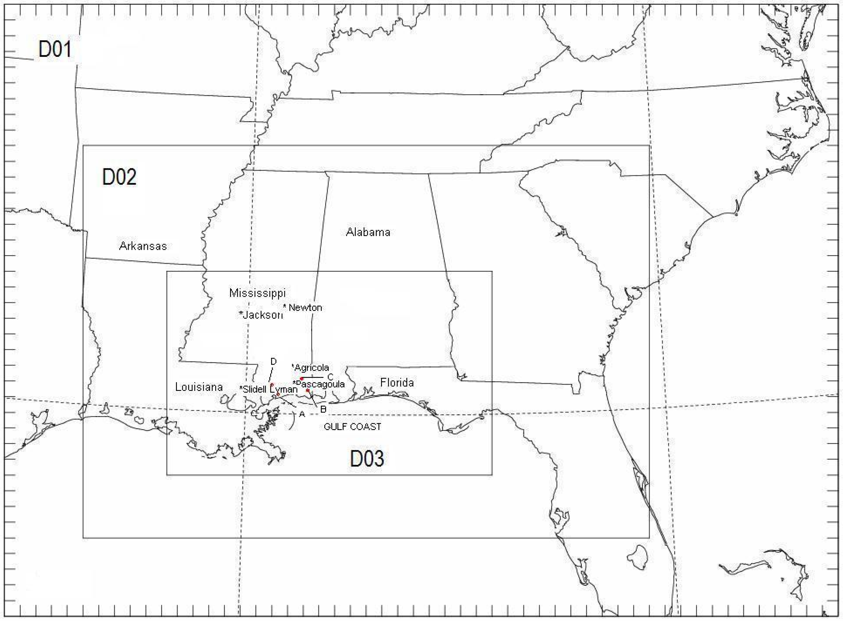
2.2. WRF Model Domains and Initialization
2.3. Dispersion Model
2.4. Dispersion Simulation
3. Results
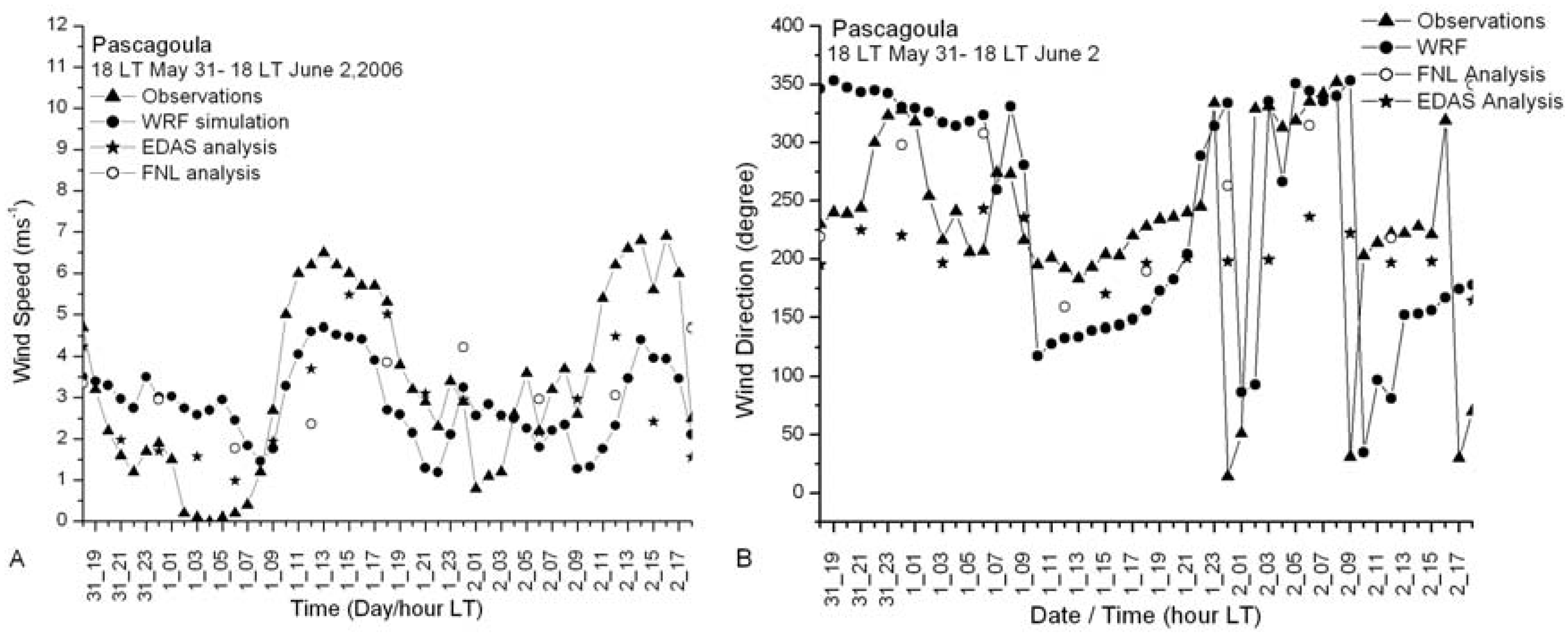
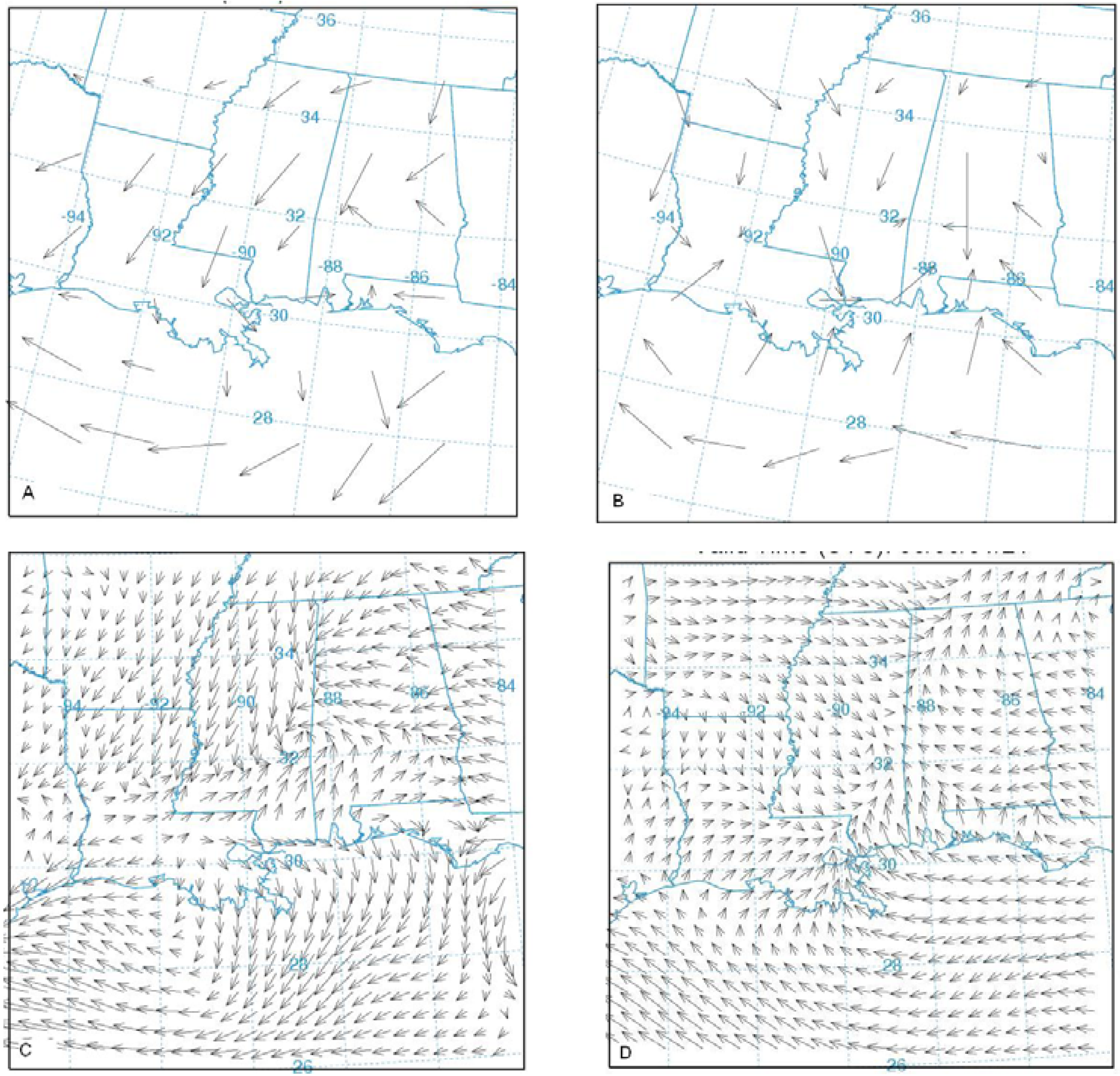
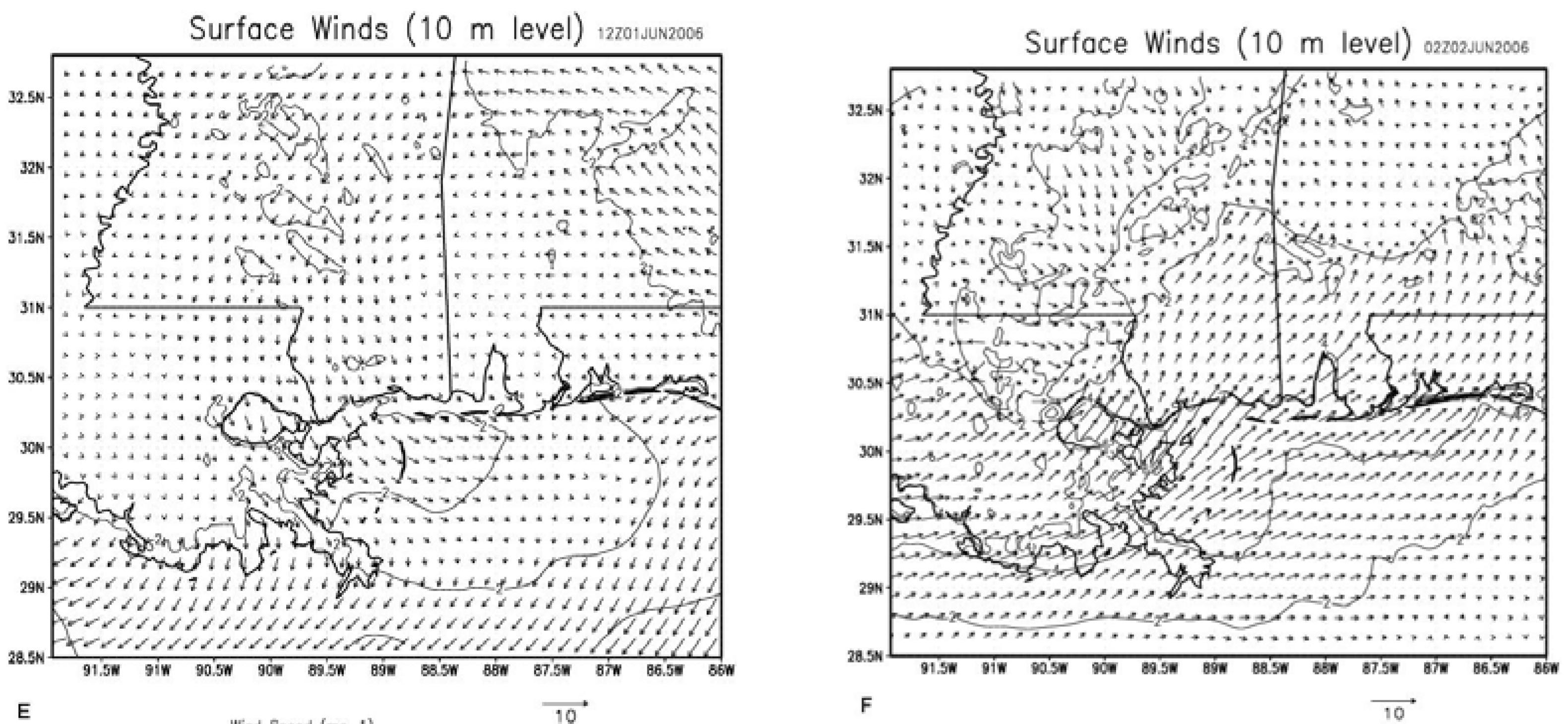
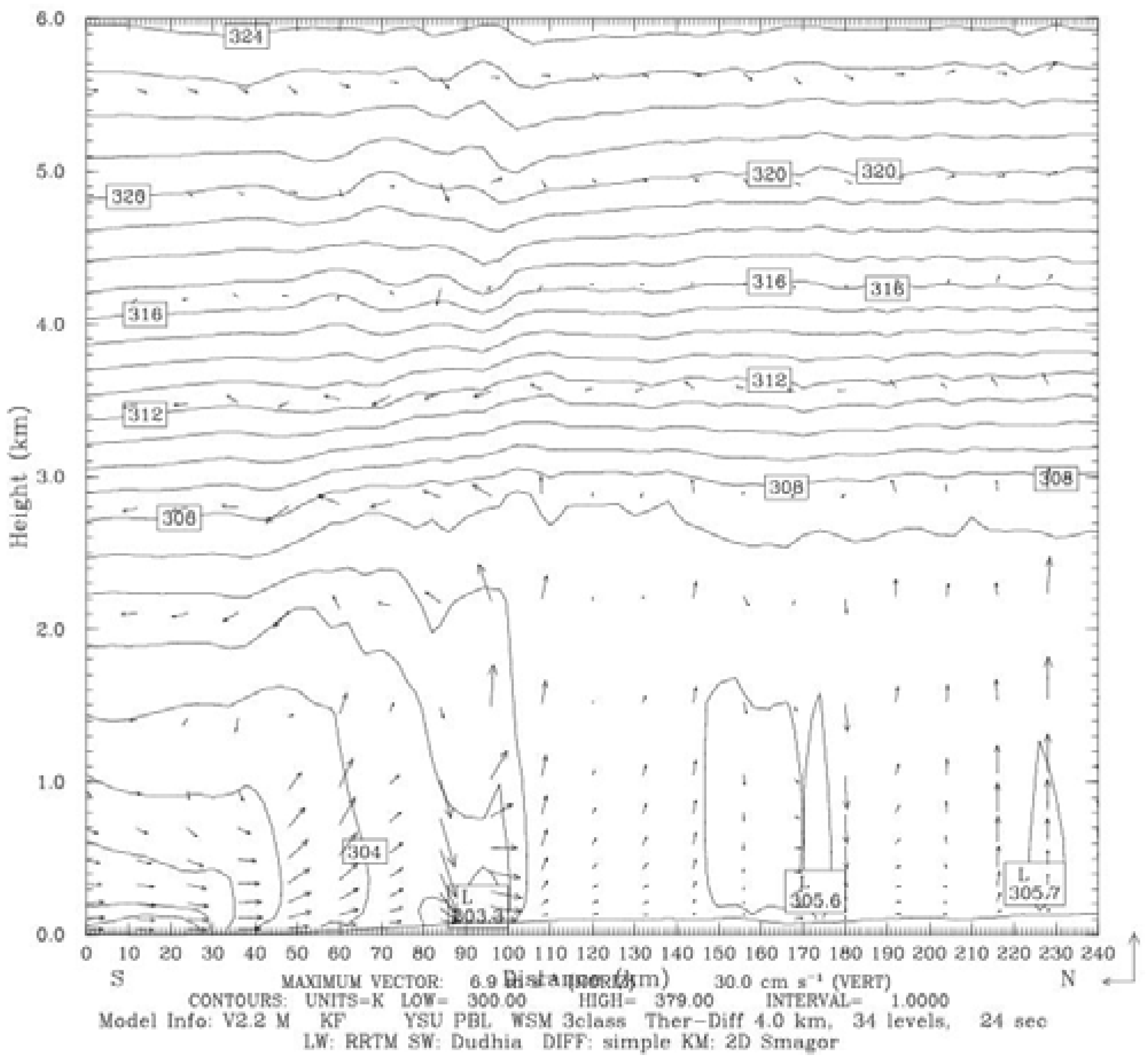
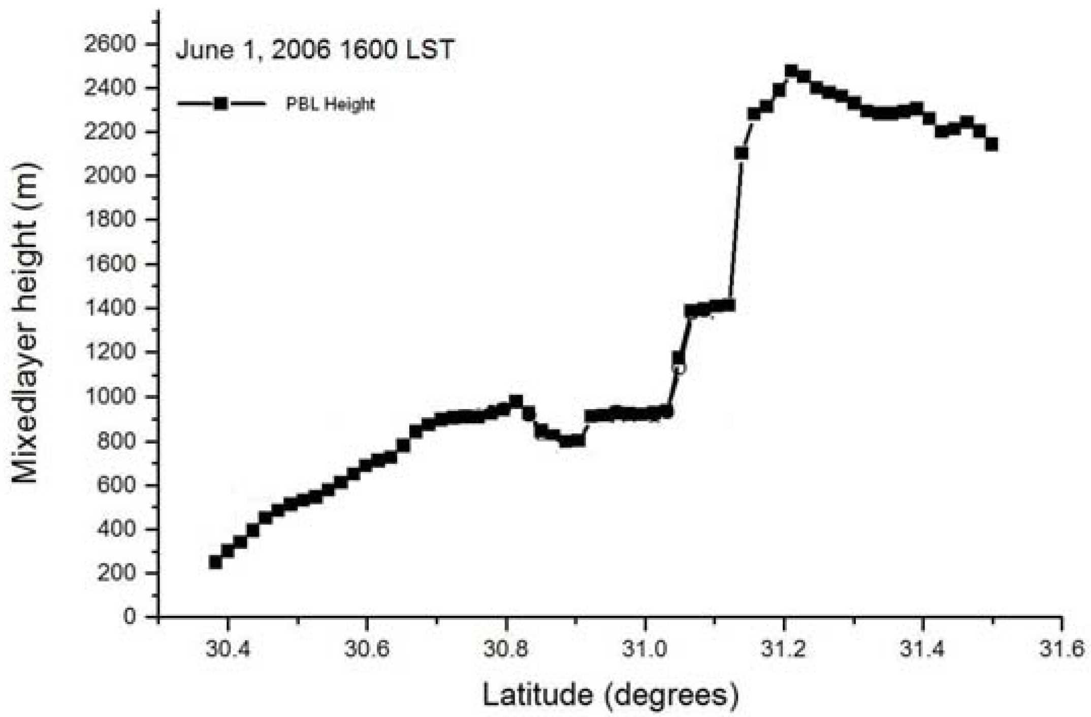
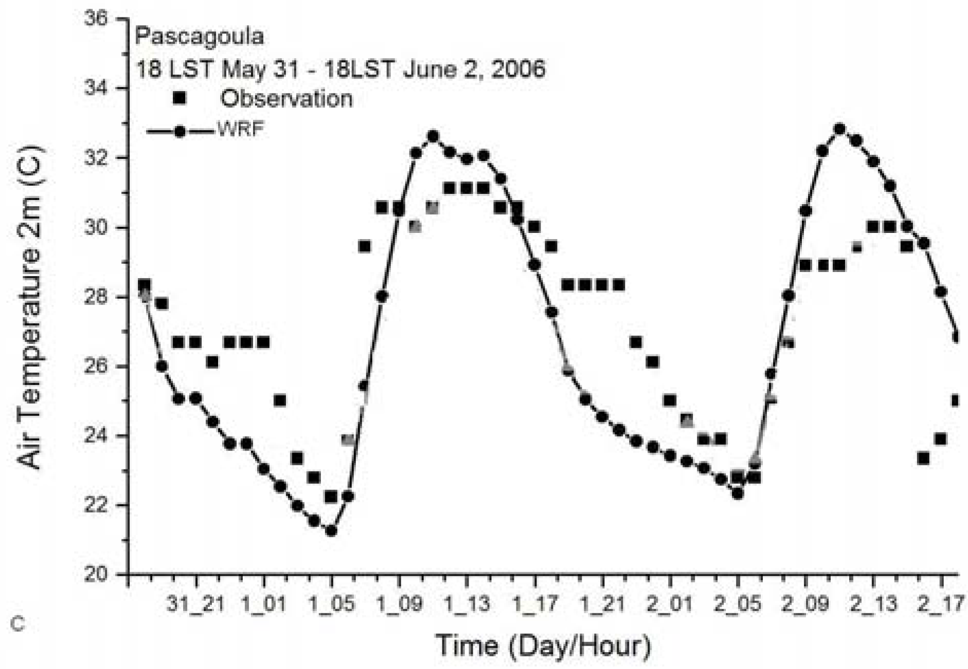
3.1. Meteorological Fields
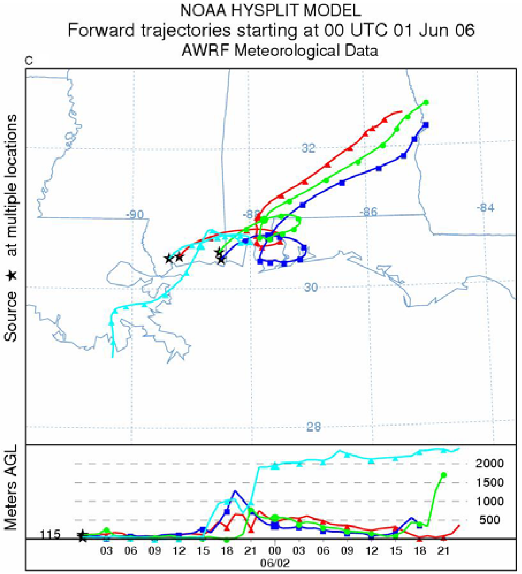
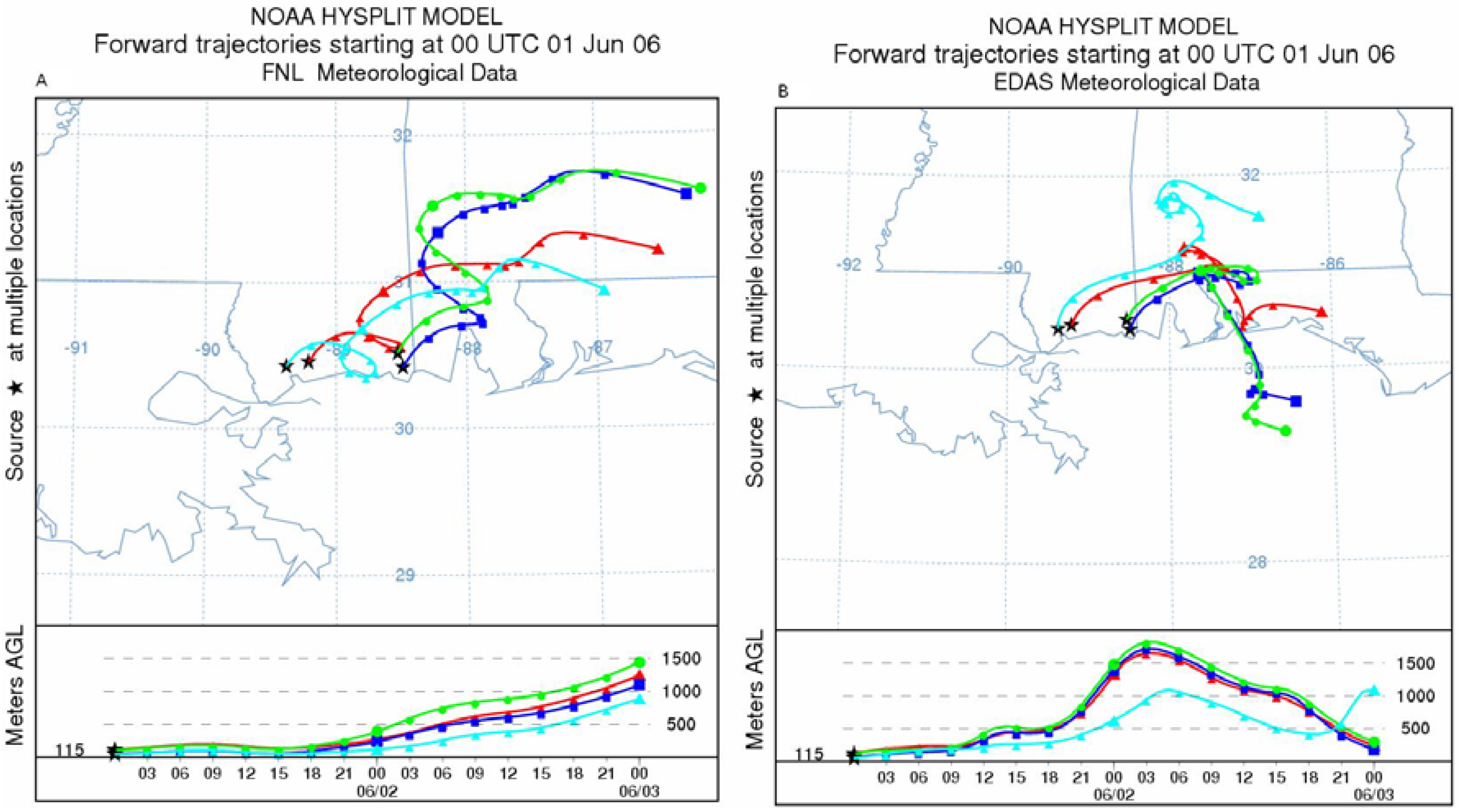
5.2 Forward Trajectories
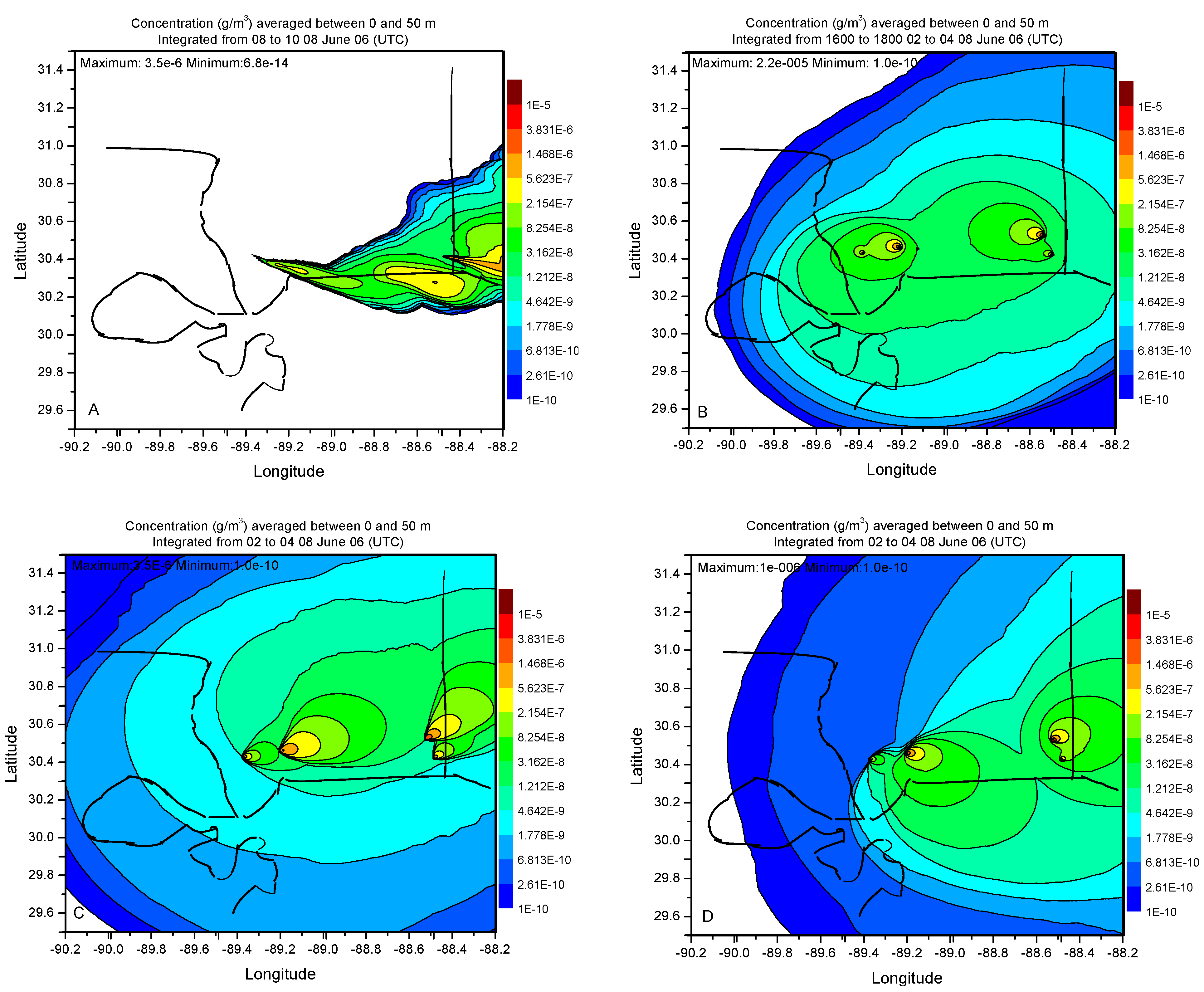
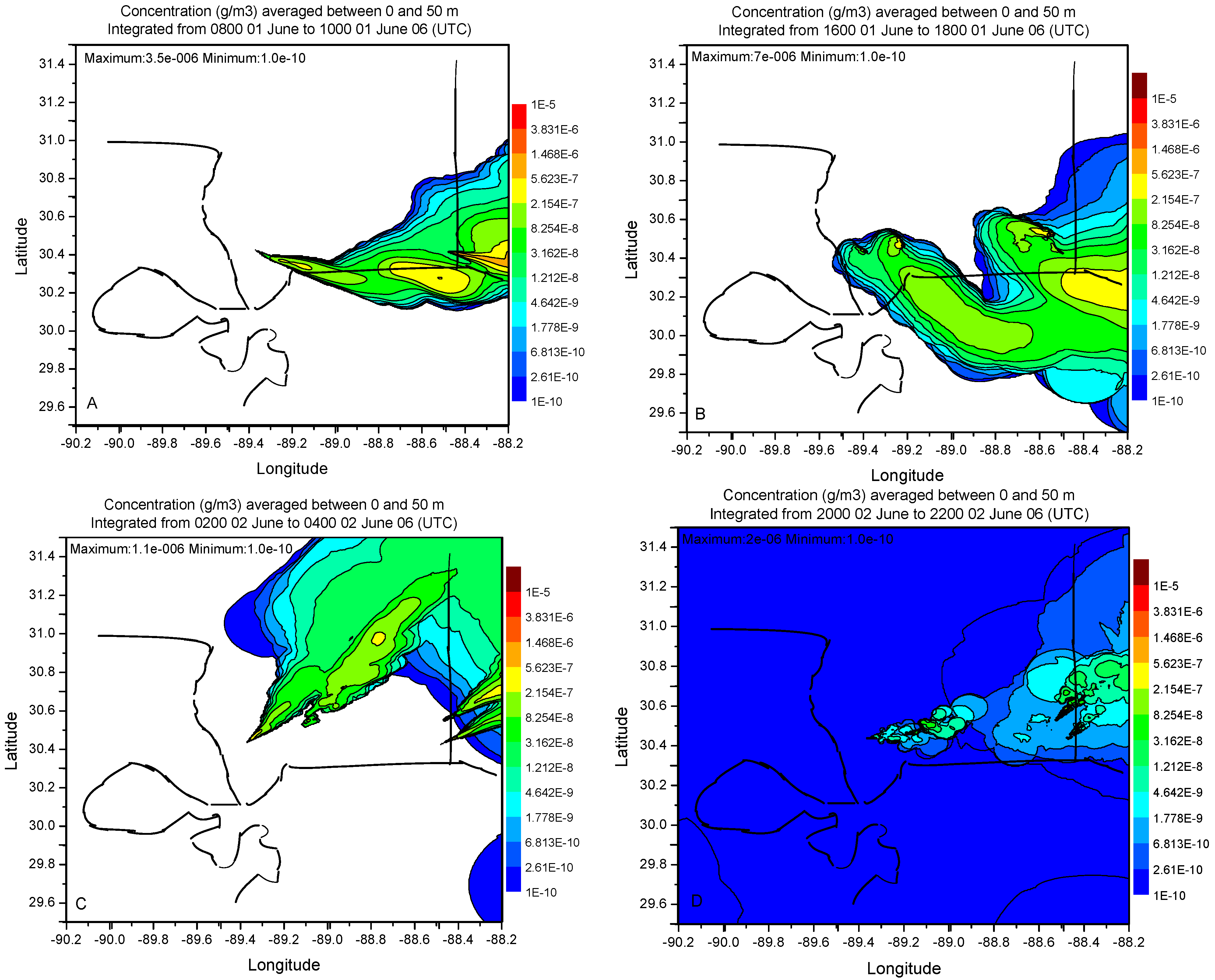
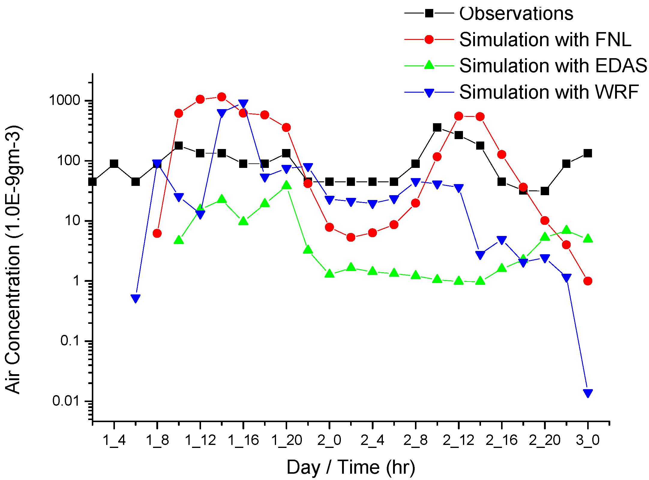
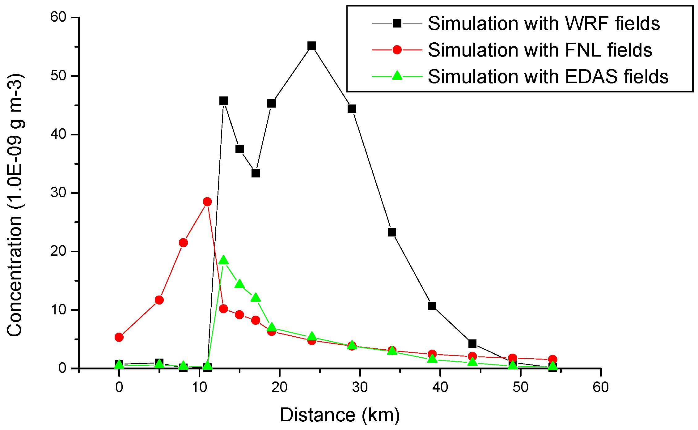
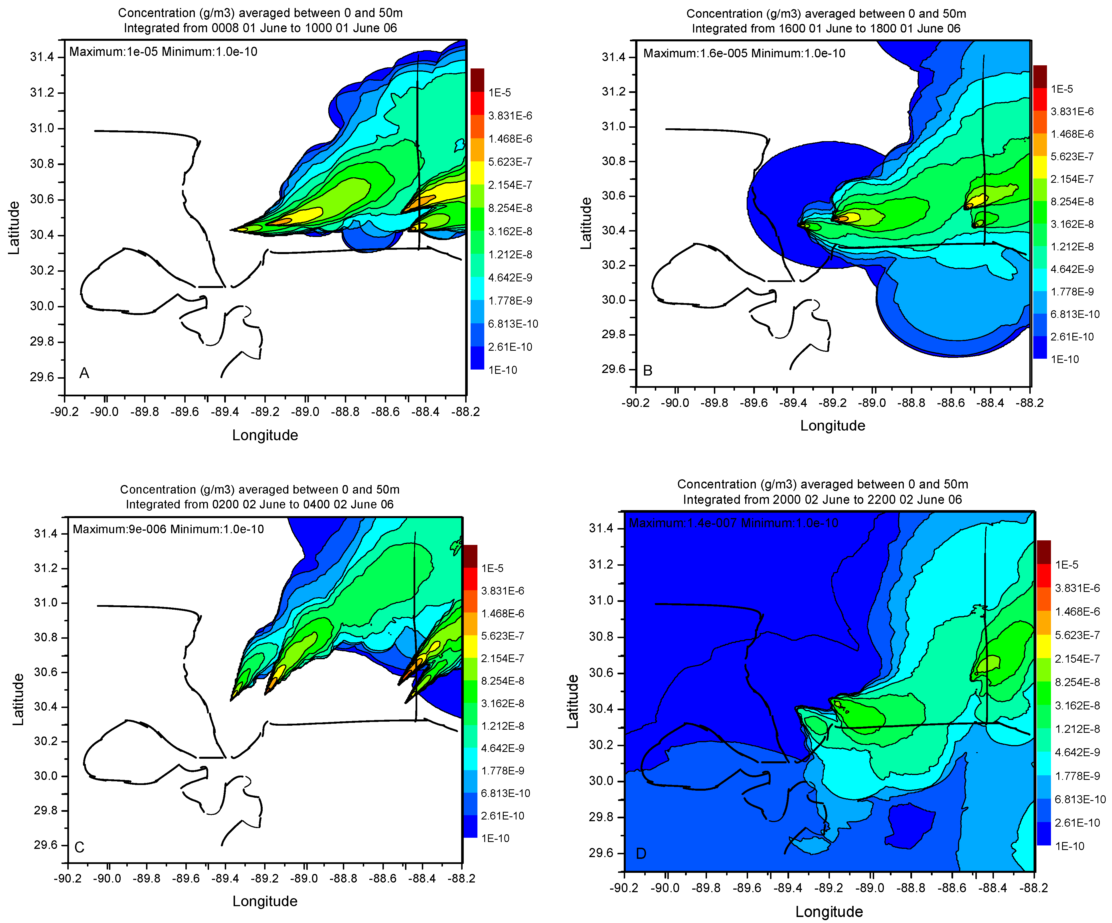
5.3. Plume Distribution Pattern
6. Conclusions
Acknowledgments
References
- Pielke, RA; Lyons, WY; McNider, RT; Moran, MD; Moon, DA; Stocker, RA; Walko, RL; Uliasz, M. Regional and Mesoscale meteorological modeling as applied to air quality studies. In Air Pollution Modeling and its Application; VIII; van Dop, H, Steyn, DG, Eds.; Plenum Press: New York, USA, 1991; pp. 259–289. [Google Scholar]
- Lu, R; Turco, RP. Air Pollutant transport in a coastal environment II. Three-dimensional simulations over Los Angeles Basin. Atmos. Env 1995, 29, 499–518. [Google Scholar]
- Luhar, AK. An analytical slab model for the growth of the coastal thermal internal boundary layer under near-neutral onshore flow conditions. Bound. Layer. Meteor 1998, 88, 103–120. [Google Scholar]
- Liu, H; Chan, JCL; Chang, AYS. Internal boundary layer structure under sea-breeze conditions in Hong Kong. Atmos. Env 2001, 35, 683–692. [Google Scholar]
- Brost, RA; Haagenson, PL; Kuo, Y-H. Eulerian simulation of tracer distribution during CAPTEX. J. Appl. Meteorol 1988, 27, 579–593. [Google Scholar]
- Warner, S; Platt, N; Heagy, JF. Comparisons of transport and dispersion model predictions of the URBAN 2000 field experiment. J. Appl. Meteor 2004, 43, 829–846. [Google Scholar]
- Nasstrom, JS; Pace, JC. Evaluation of the effect of meteorological data resolution on Lagrangian particle dispersion simulations using the Etex experiment-real-time modeling of airborne hazardous material. Atmos. Env 1998, 32, 4187–4194. [Google Scholar]
- Draxler, RR. The use of Global and Mesoscale meteorological Model data to Predict the Transport and Dispersion of Tracer Plumes over Washington, D.C. Wea. Forecasting 2006, 21, 383–394. [Google Scholar]
- Physick, WL; Abbs, DJ. Modeling of Summertime Flow and Dispersion in the Coastal Terrain of Southeastern Australia. Mon. Wea. Rev 1991, 119, 1014–1030. [Google Scholar]
- Kotroni, V; Kallos, G; Lagouvardos, K; Varinou, M. Numerical simulations of the meteorological and dispersion conditions during an air pollution episode over Anthes, Greece. J. Appl. Meteor 1999, 38, 432–447. [Google Scholar]
- Wang, G; Ostoja-Starzewski, M. A numerical study of plume dispersion motivated by a mesoscale atmospheric flow over a complex terrain. Appl. Math. Model 2004, 28, 957–981. [Google Scholar]
- Segal, M; Pielke, RA; Arritt, RW; Moran, MD; Yu, CH; Henderson, D. Application of a mesoscale atmospheric dispersion modeling system to the estimation of SO2 concentrations from major elevated sources in southern Florida. Atmos. Env 1988, 22, 1319–1334. [Google Scholar]
- Draxler, RR; Hess, GD. An overview of the HYSPLIT_4 modeling system for trajectories, dispersion and deposition. Aust. Meteor. Mag 1998, 47, 295–308. [Google Scholar]
- Black, TL. The new NMC mesoscale eta model: Description and forecast examples. Wea. Forecasting 1994, 9, 265–278. [Google Scholar]
- Rogers, E; Deaven, DG; DiMego, GJ. The regional analysis system for the operational “early” Eta model: Original 80-km configuration and recent changes. Wea. Forecasting 1995, 10, 810–825. [Google Scholar]
- Rogers, E; Black, TL; Deaven, DG; DiMego, GJ; Zhao, Q; Baldwin, MN; Junker, W; Lin, Y. Changes to the operational “early” Eta analysis/forecast system at the National Centers for Environmental Prediction. Wea. Forecasting 1996, 11, 391–413. [Google Scholar]
- Challa, VS; Indracanti, J; Rabarison, MK; Patrick, C; Baham, JM; Young, J; Hughes, R; Hardy, MG; Swanier, SJ; Anjaneyulu, Y. A simulation study of mesoscale coastal circulations in Mississippi Gulf coast. Atmos. Res 2009, 91, 9–25. [Google Scholar]
- Skamarock, WC; Klemp, J; Dudhia, J; Gill, DO; Barker, DM; Wang, W; Powers, JG. A Description of the Advanced Research WRF Version 2; NCAR Technical Note, NCAR/TN-468+STR, Mesoscale and Microscale Meteorology DivisionNational Center for Atmospheric Research: Boulder, Colorado, USA, 2005; pp. 1–113. [Google Scholar]
- Kain, JS; Fritsch, JM. Convective parameterization for mesoscale models: The Kain-Fritcsh scheme. In The representation of cumulus convection in numerical models; Emanuel, KA, Raymond, DJ, Eds.; American Meteorological Society: Boston, MA, USA, 1993. [Google Scholar]
- Hong, SY; Dudhia, J; Chen, SH. A Revised Approach to Ice Microphysical processes for the Bulk Parameterization of Clouds and Precipitation. Mon. Wea. Rev 2004, 132, 103–120. [Google Scholar]
- Hong, SY; Noh, Y; Dudhia, J. A new vertical diffusion package with explicit treatment of entrainment processes. Mon. Wea. Rev 2006, 134, 2318–2341. [Google Scholar]
- Dudhia, J. A multi-layer soil temperature model for MM5. In Preprints, Sixth PSU/NCAR Mesonet Model Users’ Workshop; PSU/NCAR: Boulder, CO, USA, 1996; pp. 49–50. [Google Scholar]
- Dudhia, J. Numerical study of convection observed during winter monsoon experiment using a mesoscale two-dimensional model. J. Atmos. Sci 1989, 46, 3077–3107. [Google Scholar]
- Mlawer, EJ; Taubman, SJ; Brown, PD; Iacono, MJ; Clough, SA. Radiative transfer for inhomogeneous atmosphere: RRTM, a validated correlated-k model for the longwave. J. Geophys. Res 1997, 102, 16663–16682. [Google Scholar]
- Seaman, NL; Stauffer, DR; Lario, AM. A multiscale four-dimensional data assimilation system applied in the San Joaquin Valley during SARMAP Part I: Modeling design and basic performance characteristics. J. Appl. Meteor 1995, 34, 1739–1761. [Google Scholar]
- Stauffer, DR; Seaman, NL. Use of four-dimensional data assimilation in a limited-area mesoscale model. Part I: Experiments with synoptic-scale data. Mon. Wea. Rev 1990, 118, 1250–1277. [Google Scholar]
- Stauffer, DR; Seaman, NL; Binkowski, F. Use of four-dimensional data assimilation in a limited-area mesoscale model. Part II-Effects of data assimilation within the planetary boundary layer. Mon. Wea. Rev 1991, 119, 734–754. [Google Scholar]


| Dynamics Vertical resolution | Primitive equation, non-hydrostatic
35 levels | ||
| Domains | Domain1 | Domain2 | Domain3 |
| Horizontal resolution | 36 km | 12 km | 4 km |
| Grid points | 54 × 40 | 109 × 76 | 187 × 118 |
| Domains of integration | 93.0 W – 78.05 E
27.16 N – 34.45 N | 91.74 W – 81.92 W
28.5 N – 34.45 N | 90.28 W – 84.77 W
29.38 N – 32.54 N |
| Radiation | Dudhia (1989) scheme for short wave radiation, Rapid radiative transfer model (RRTM) for long wave radiation | ||
| Surface processes | 5 layer soil diffusion scheme | ||
| Boundary layer | Yonsei State University (YSU) PBL scheme | ||
| Sea surface temperature | NCEP FNL analysis data | ||
| Convection | Kain and Fritsch scheme on the outer grids domain1, domain2 | ||
| Explicit moisture | WSM3 class simple ice (SI) scheme | ||
| Elevated Source Location | Source | Latitude / Longitude | Stack Height Hs (m) | Stack Diameter Ds (m) | Source strength Qs (g s−1) |
|---|---|---|---|---|---|
| Gulfport (A) | Mississippi Power
Plant Jack Wa | 30.46° N; −89.21° E | 115.12 | 3.85 | 24,869.5 |
| Pascagoula (B) | Chevron Products
Pascagoula Refinery | 30.42° N: −88.49° E | 54.1 | 1.35 | 1,742.8 |
| Escatawpa (C) | Mississippi Power
Plant Victor | 30.52° N; −88.53° E | 105.0 | 10.23 | 12,522.2 |
| Passchritian (D) | Dupont Delisle
Facility | 30.43° N; −89.38° E | 45.0 | 3.0 | 1,270.5 |
| Model version | 4.8 |
| Grid Centre | 30.5 N, −89.5 L |
| Vertical resolution | 8 Levels – 25, 50, 100, 200, 500, 1000, 2000, 5000 |
| Horizontal Grid | 2 × 2 degree |
| Horizontal resolution | 0.01 × 0.01 |
| Turbulence Method | Standard Velocity Deformation |
| Meteorology | NCEP FNL 6 h data, EDAS 3 h data,
WRF Simulated hourly meteorological fields |
| Frequency of emissions cycle | 500 particles per hour |
| Data Used | Time (UTC) | Statistics of dispersion calculation (units : g/m3)
| |||||
|---|---|---|---|---|---|---|---|
| Mean | S.D | S.E | Min | Max | Range | ||
| FNL | 08–10 June 01 | 1.01E-08 | 5.43E-08 | 1.35E-10 | 0.0 | 3.28E-06 | 3.28E-06 |
| 16–18 June 01 | 8.90E-09 | 8.91E-08 | 2.22E-10 | 0.0 | 2.05E-05 | 2.05E-05 | |
| 02–04 June 02 | 1.27E-08 | 5.96E-08 | 1.49E-10 | 0.0 | 3.32E-06 | 3.32E-06 | |
| 20–22 June 02 | 8.53E-09 | 6.19E-08 | 1.54E-10 | 0.0 | 1.15E-05 | 1.15E-05 | |
| ETA AWIP | 08–10 June 01 | 8.73E-09 | 5.81E-08 | 1.45E-10 | 0.0 | 9.70E-06 | 9.70E-06 |
| 16–18 June 01 | 5.69E-09 | 6.64E-08 | 1.66E-10 | 0.0 | 1.45E-05 | 1.45E-05 | |
| 02–04 June 02 | 6.42E-09 | 6.74E-08 | 1.68E-10 | 0.0 | 8.17E-06 | 8.17E-06 | |
| 20–22 June 02 | 3.11E-09 | 9.12E-09 | 2.27E-11 | 0.0 | 1.24E-07 | 1.24E-07 | |
| WRF | 08–10June 01 | 1.01E-08 | 5.43E-08 | 1.35E-10 | 0.0 | 3.28E-06 | 3.28E-06 |
| 16–18 June 01 | 1.43E-08 | 5.72E-08 | 1.43E-10 | 0.0 | 6.93E-06 | 6.93E-06 | |
| 02–04 June 02 | 7.28E-09 | 2.53E-08 | 6.32E-11 | 0.0 | 1.01E-06 | 1.01E-06 | |
| 20–22 June 02 | 5.47E-10 | 1.01E-08 | 2.51E-11 | 0.0 | 1.95E-06 | 1.95E-06 | |
| Meteorological data | R | FB (24 h) | FB (8 h day) | FB (8 h night) |
|---|---|---|---|---|
| FNL | 0.396 | 0.81 | 1.47 | −1.04 |
| EDAS | 0.10 | −1.33 | −1.39 | −1.85 |
| WRF mesoscale simulation | 0.21 | −0.82 | −1.47 | −0.41 |
© 2009 by the authors; licensee Molecular Diversity Preservation International, Basel, Switzerland. This article is an open-access article distributed under the terms and conditions of the Creative Commons Attribution license (http://creativecommons.org/licenses/by/3.0/).
Share and Cite
Yerramilli, A.; Srinivas, C.V.; Dasari, H.P.; Tuluri, F.; White, L.D.; Baham, J.; Young, J.H.; Hughes, R.; Patrick, C.; Hardy, M.G.; et al. Simulation of Atmospheric Dispersion of Elevated Releases from Point Sources in Mississippi Gulf Coast with Different Meteorological Data. Int. J. Environ. Res. Public Health 2009, 6, 1055-1074. https://doi.org/10.3390/ijerph6031055
Yerramilli A, Srinivas CV, Dasari HP, Tuluri F, White LD, Baham J, Young JH, Hughes R, Patrick C, Hardy MG, et al. Simulation of Atmospheric Dispersion of Elevated Releases from Point Sources in Mississippi Gulf Coast with Different Meteorological Data. International Journal of Environmental Research and Public Health. 2009; 6(3):1055-1074. https://doi.org/10.3390/ijerph6031055
Chicago/Turabian StyleYerramilli, Anjaneyulu, Challa Venkata Srinivas, Hari Prasad Dasari, Francis Tuluri, Loren D. White, Julius Baham, John H. Young, Robert Hughes, Chuck Patrick, Mark G. Hardy, and et al. 2009. "Simulation of Atmospheric Dispersion of Elevated Releases from Point Sources in Mississippi Gulf Coast with Different Meteorological Data" International Journal of Environmental Research and Public Health 6, no. 3: 1055-1074. https://doi.org/10.3390/ijerph6031055