Variation of Natural Streamflow since 1470 in the Middle Yellow River, China

Abstract
:1. Introduction
2. Materials and Methods
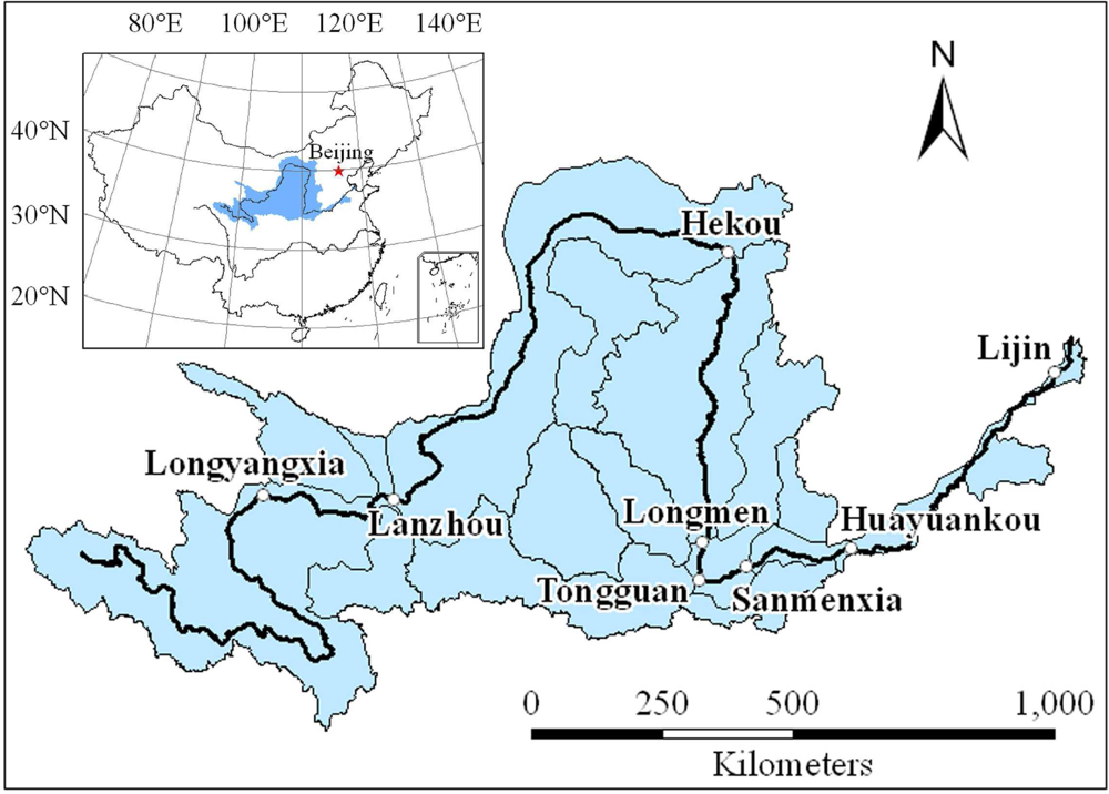
2.1. Study Area
2.2. Data Collect
2.3. Analysis Methods
(1) Statistical analysis
(2) Low flow analysis
(3) Mann-Kendall test
(4) Wavelet analysis
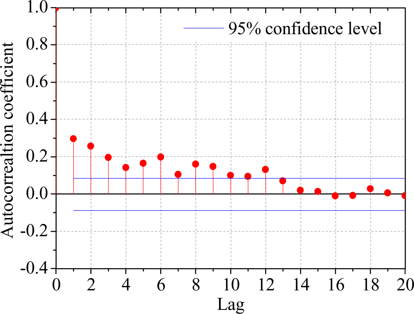
2.4. Data Preliminary Analysis
3. Results
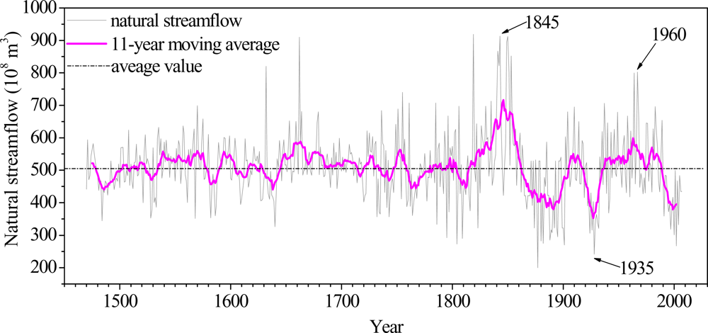
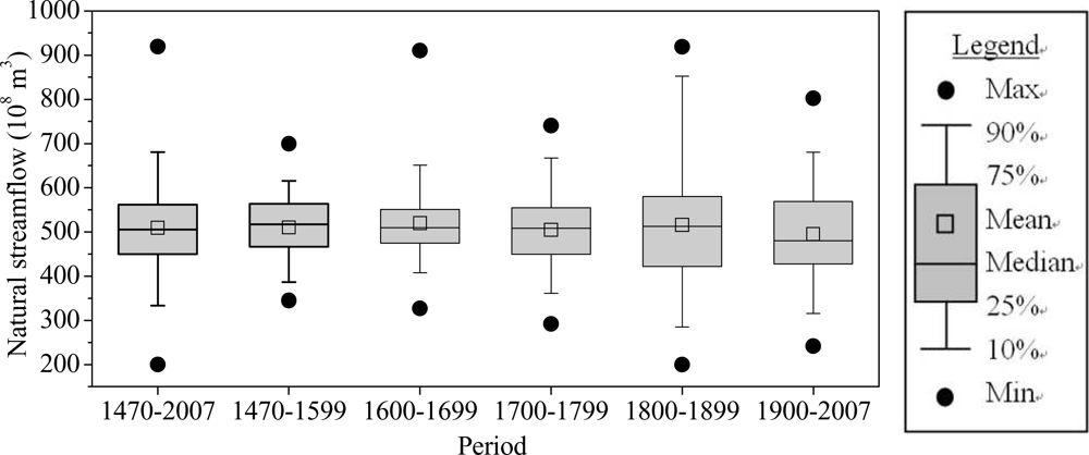
3.1. Statistical Characteristics
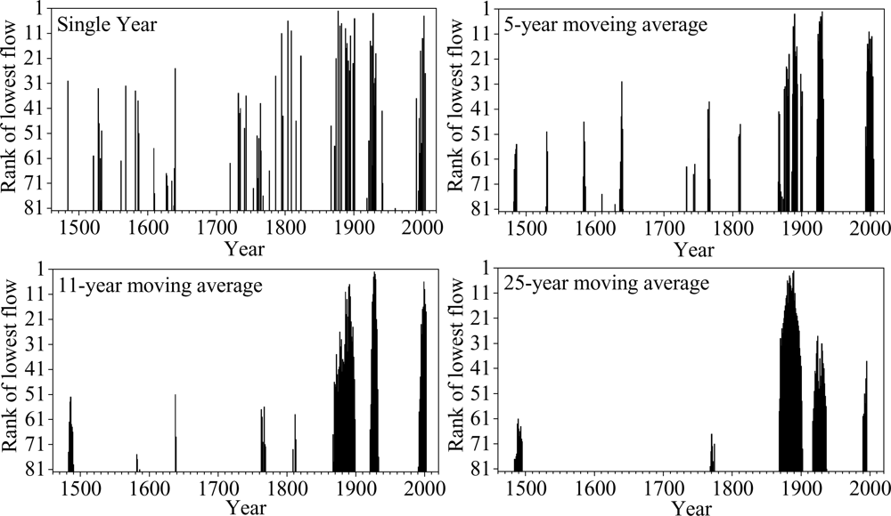
3.2. Drought Events
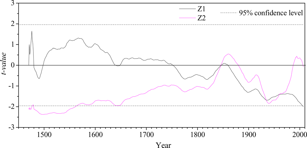
3.3. Mann-Kendall Test
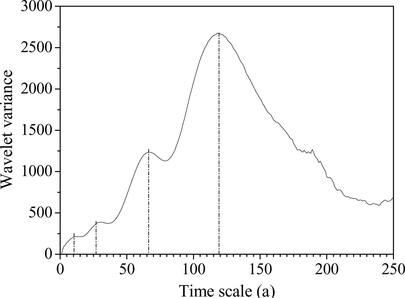
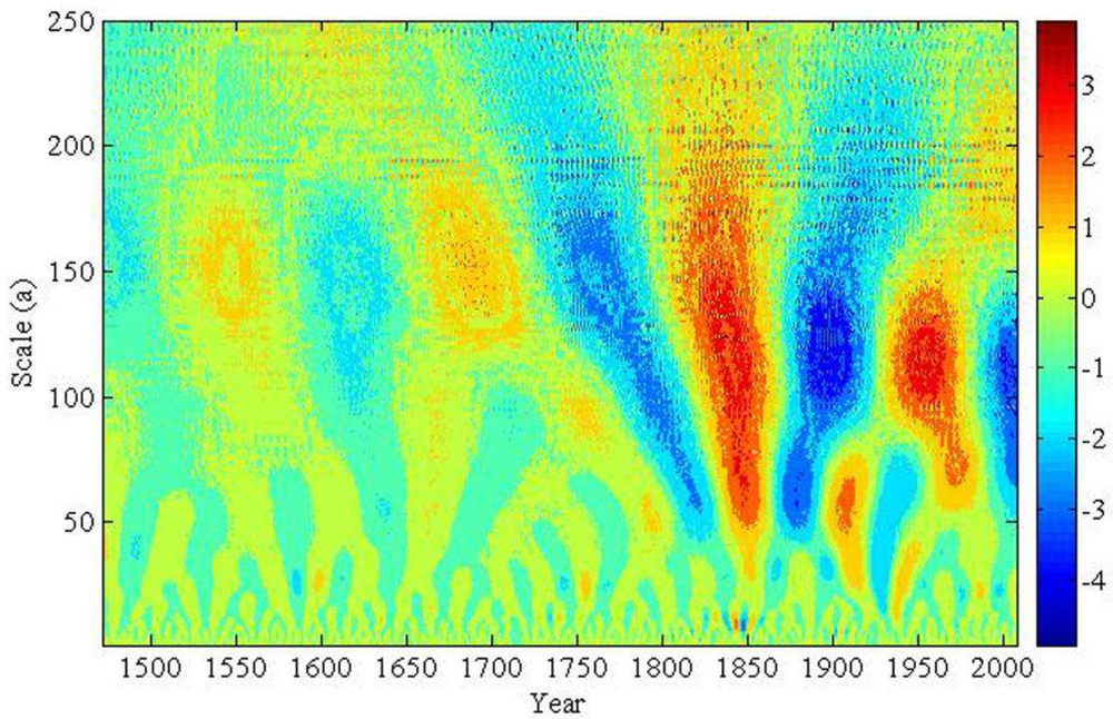
3.4. Wavelet Transform
4. Discussion
5. Conclusions
Acknowledgments
References
- Zhang, XH; Zhang, HW; Chen, B; Chen, GQ; Zhao, XH. Water resources planning based on complex system dynamics: A case study of Tianjin city. Commun. Nonlinear Sci. Numer. Simul 2008, 13, 2328–2336. [Google Scholar]
- Yang, ZF; Sun, T; Cui, BS; Chen, B; Chen, GQ. Environmental flow requirements for integrated water resources allocation in the Yellow River basin, China. Commun. Nonlinear Sci. Numer. Simul 2009, 14, 2469–2481. [Google Scholar]
- Williams, GR. Cyclical variations in the world-wide hydrological data. J. Hydraul. Div 1961, 6, 71–88. [Google Scholar]
- Currie, RG. Variance contribution of luni-solar (Mn) and solar cycle (Sc) signals to climate data. Int. J. Climatol 1996, 16, 1343–1364. [Google Scholar]
- Probst, J; Tardy, Y. Long range streamflow and world continental runoff fluctuation since the beginning of this century. J. Hydrol 1987, 94, 289–311. [Google Scholar]
- Whitfield, PH. Linked hydrologic and climate variations in British Columbia and Yukon. Environ. Monit. Assess 2001, 67, 217–238. [Google Scholar]
- Woodhouse, CA. A tree-ring reconstruction of streamflow for the Colorado front range. J. Am. Water Resour. As 2001, 37, 561–569. [Google Scholar]
- Gedalof, Z; Peterson, DL; Mantua, NJ. Columbia river flow and drought since 1750. J. Am. Water Resour. As 2004, 40, 1579–1592. [Google Scholar]
- Absalon, D; Matysik, M. Changes in water quality and runoff in the Upper Oder River basin. Geomorphology 2007, 92, 106–118. [Google Scholar]
- Sen, AK. Spectral-temporal characterization of riverflow variability in England and Wales for the period 1865–2002. Hydrol. Process 2009, 23, 1147–1157. [Google Scholar]
- Zhang, Q; Xu, CY; Becker, S; Tong, J. Sediment and runoff changes in the Yangtze River basin during past 50 years. J. Hydrol 2006, 331, 511–523. [Google Scholar]
- Xu, JJ; Yang, DW; Yi, YH; Lei, ZD; Chen, J; Yang, WJ. Spatial and temporal variation of runoff in the Yangtze River basin during the past 40 years. Quat. Int 2008, 186, 32–42. [Google Scholar]
- Jiang, T; Su, BD; Hartmann, HK. Temporal and spatial trends of precipitation and river flow in the Yangtze River basin, 1961–2000. Geomorphology 2007, 85, 143–154. [Google Scholar]
- Zhang, Q; Liu, CL; Xu, CY; Xu, YP; Jiang, T. Observed trends of annual maximum water level and streamflow during past 130 years in the Yangtze River basin, China. J. Hydrol 2006, 324, 255–265. [Google Scholar]
- Hu, Q; Feng, S. A southward migration of centennial-scale variation of drought/flood in eastern China and the western United States. J. Clim 2001, 14, 1323–1328. [Google Scholar]
- Qian, W; Zhu, Y. Climate change in China from 1880 to 1998 and its impact on the environmental condition. Clim. Change 2001, 50, 419–444. [Google Scholar]
- Zheng, HX; Zhang, L; Liu, CM; Shao, QX; Fukushima, Y. Changes in stream flow regime in headwater catchments of the Yellow River basin since the 1950s. Hydrol. Process 2007, 21, 886–893. [Google Scholar]
- Xu, JX. Temporal variation of river flow renewability in the middle Yellow River and the influencing factors. Hydrol. Process 2005, 19, 1871–1882. [Google Scholar]
- Wu, BS; Wang, GQ; Xia, JQ; Fu, XD; Zhang, YF. Response of bankfull discharge to discharge and sediment load in the Lower Yellow River. Geomorphology 2008, 100, 366–376. [Google Scholar]
- Wang, SJ; Hassan, MA; Xie, XP. Relationship between suspended sediment load, channel geometry and land area increment in the Yellow River delta. Catena 2006, 65, 302–314. [Google Scholar]
- Li, CH; Yang, ZF; Huang, GH; Li, YP. Identification of relationship between sunspots and natural runoff in the Yellow River based on discrete wavelet analysis. Expert Syst. Appl 2009, 36, 3309–3318. [Google Scholar]
- Chen, B; Chen, GQ; Hao, FH; Yang, ZF. Exergy-based water resource allocation of the mainstream Yellow River. Commun. Nonlinear Sci. Numer. Simul 2009, 14, 1721–1728. [Google Scholar]
- Wang, GA; Shi, FC; Zheng, XY; Gao, ZD; Yi, YJ; Ma, GA; Mu, P. Natural annual runoff estimation from 1470 to 1918 for Sanmenxia gauge station of Yellow River. Adv Water Sci 1999, 10, 170–176. (in Chinese).. [Google Scholar]
- Chinese Academy of Meteorological Sciences (CAMS). Maps of the Drought and Flood Distribution of China in Recent 500 Years; Map Press: Beijing, China, 1981; pp. 17–39. (in Chinese). [Google Scholar]
- Mann, HB. Nonparametric tests against trend. Econometrica 1945, 13, 245–259. [Google Scholar]
- Kendall, MG. Rank Correlation Methods; Charles Griffin: London, UK, 1975. [Google Scholar]
- Serrano, VL; Mateos, VL; García, JA. Trend analysis of monthly precipitation over the Iberian Peninsula for the period 1921–1995. Phys. Chem. Earth-B 1999, 24, 85–90. [Google Scholar]
- Mitchell, JM; Dzerdzeevskii, B; Flohn, H; Hofmeyr, WL; Lamb, HH; Rao, KN; Wallén, CC. Climate Change; WMO Technical Note No.79, World Meteorological Organization: Geneva, Switzerland, 1966. [Google Scholar]
- Gerstengarbe, FW; Werner, PC. Estimation of the beginning and end of recurrent events within a climate regime. Climate Res 1999, 11, 97–107. [Google Scholar]
- Nakken, M. Wavelet analysis of rainfall-runoff variability isolating climatic from anthropogenic patterns. Environ. Modell. Softw 1999, 14, 283–295. [Google Scholar]
- Matalas, NC; Langbein, WB. Information content of the mean. J. Geophys. Res 1962, 67, 3441–3448. [Google Scholar]
- Yue, S; Wang, CY. The Mann-Kendall test modified by effective sample size to detect trend in serially correlated hydrological series. Water Resour. Manag 2004, 18, 201–218. [Google Scholar]
- Yue, S; Pilon, P; Phinney, B; Cavadias, G. The influence of autocorrelation on the ability to detect trend in hydrological series. Hydrol. Process 2002, 16, 1807–1829. [Google Scholar]
- Pandit, SM; Wu, SM. Time Series and System Analysis with Applications; John Wiley & Sons, Inc: NewYork, NY, USA, 1983; pp. 72–97. [Google Scholar]
- Wang, YZ; Liu, WL. Relations of ice and snow of the South Pole and amount of runoff of the Yellow River. Yellow River 1988, 4, 22–26. (in Chinese).. [Google Scholar]
- Mechoso, CR; Iribarren, GP. Streamflow in Southeastern America and the Southern Oscillation. J. Climate 1992, 5, 1535–1539. [Google Scholar]
- Xu, ZX; Chen, YN; Li, JY. Impact of climate change on water resources in the Tarim river basin. Water Resour. Manag 2004, 18, 439–458. [Google Scholar]
- Gong, DY; Wang, SW. Impact of ENSO on global precipitation and precipitation in China during past 100 years. Chinese Sci. Bull 1999, 44, 315–320. [Google Scholar]


© 2009 by the authors; licensee Molecular Diversity Preservation International, Basel, Switzerland. This article is an open-access article distributed under the terms and conditions of the Creative Commons Attribution license (http://creativecommons.org/licenses/by/3.0/).
Share and Cite
Miao, C.-Y.; Ni, J.-R. Variation of Natural Streamflow since 1470 in the Middle Yellow River, China. Int. J. Environ. Res. Public Health 2009, 6, 2849-2864. https://doi.org/10.3390/ijerph6112849
Miao C-Y, Ni J-R. Variation of Natural Streamflow since 1470 in the Middle Yellow River, China. International Journal of Environmental Research and Public Health. 2009; 6(11):2849-2864. https://doi.org/10.3390/ijerph6112849
Chicago/Turabian StyleMiao, Chi-Yuan, and Jin-Ren Ni. 2009. "Variation of Natural Streamflow since 1470 in the Middle Yellow River, China" International Journal of Environmental Research and Public Health 6, no. 11: 2849-2864. https://doi.org/10.3390/ijerph6112849