Seasonal Variation of Water Quality in Unregulated Domestic Wells

 ,
,  , and
, and
Abstract
:
1. Introduction
2. Materials and Methods
2.1. Recruitment
2.2. Determination of Wet and Dry Seasons
2.3. Sample Collection
2.4. Analysis of Microbial Contaminants
2.5. Analysis of Inorganic Contaminants
2.6. Analysis of Organic Contaminants
2.7. Data Analysis
3. Results
3.1. Sampled Population Characteristcs
3.2. Water Quality Parameters
3.3. Summary of Contaminants in Water Samples
4. Discussion
5. Conclusions
Author Contributions
Funding
Acknowledgments
Conflicts of Interest
References
- Hutson, S.S.; Barber, N.L.; Kenny, J.F.; Linsey, K.S.; Lumia, D.S.; Maupin, M.A. Estimated Use of Water in the United States in 2000. U.S. Geological Survey Circular 1268; U.S. Geological Survey: Denver, CO, USA, 2004.
- Allevi, R.P.; Krometis, L.-A.H.; Hagedorn, C.; Benham, B.; Lawrence, A.H.; Ling, E.J.; Ziegler, P.E. Quantitative analysis of microbial contamination in private drinking water supply systems. J. Water Health 2013, 11, 244–255. [Google Scholar] [CrossRef]
- Buragohain, M.; Bhuyan, B.; Sarma, H.P. Seasonal variations of lead, arsenic, cadmium and aluminium contamination of groundwater in Dhemaji district, Assam, India. Environ. Monit Assess. 2010, 170, 345–351. [Google Scholar] [CrossRef] [PubMed]
- Messier, K.P.; Kane, E.; Bolich, R.; Serre, M.L. Nitrate Variability in Groundwater of North Carolina using Monitoring and Private Well Data Models. Environ. Sci. Technol. 2014, 48, 10804–10812. [Google Scholar] [CrossRef] [PubMed]
- Flanagan, S.V.; Spayd, S.E.; Procopio, N.A.; Chillrud, S.N.; Ross, J.; Braman, S.; Zheng, Y. Arsenic in private well water part 2 of 3: Who benefits the most from traditional testing promotion? Sci. Total Environ. 2016, 562, 1010–1018. [Google Scholar] [CrossRef]
- Flanagan, S.V.; Marvinney, R.G.; Zheng, Y. Influences on domestic well water testing behavior in a Central Maine area with frequent groundwater arsenic occurrence. Sci. Total Environ. 2015, 505, 1274–1281. [Google Scholar] [CrossRef]
- Imgrund, K.; Kreutzwiser, R.; De Loë, R. Influences on the water testing behaviors of private well owners. J. Water Health 2011, 9, 241–252. [Google Scholar] [CrossRef] [Green Version]
- Sanders, A.P.; A Desrosiers, T.; Warren, J.L.; Herring, A.H.; Enright, D.; Olshan, A.F.; E Meyer, R.; Fry, R.C. Association between arsenic, cadmium, manganese, and lead levels in private wells and birth defects prevalence in North Carolina: A semi-ecologic study. BMC Water Health 2014, 14, 955. [Google Scholar]
- Schaider, L.A.; Ackerman, J.M.; Rudel, R.A. Septic systems as sources of organic wastewater compounds in domestic drinking water wells in a shallow sand and gravel aquifer. Sci. Total Environ. 2016, 547, 470–481. [Google Scholar] [CrossRef] [Green Version]
- Swistock, B.R.; Sharpe, E.W. The influence of well construction on bacterial contamination of private water wells in Pennsylvania. J. Environ. Health 2005, 68, 17–22. [Google Scholar]
- Won, G.; Gill, A.; Lejeune, J.T. Microbial quality and bacteria pathogens in private wells used for drinking water in northeastern Ohio. J. Water Health 2013, 11, 555–562. [Google Scholar] [CrossRef]
- Yates, M.V. Septic tank density and ground water contamination. Ground Water 1985, 23, 586–591. [Google Scholar] [CrossRef]
- Choudhury, I.; Ahmed, K.M.; Hasan, M.; Mozumder, M.R.H.; Knappett, P.S.K.; Ellis, T.; Van Geen, A. Evidence for Elevated Levels of Arsenic in Public Wells of Bangladesh Due to Improper Installation. Ground Water 2016, 54, 871–877. [Google Scholar] [CrossRef] [PubMed]
- DeSimone, L.; Hamilton, P.; Gilliom, R. The Quality of Our Nation’s Waters—Quality of Water from Domestic Wells in Principal Aquifers of the United States, 1991–2004—Overview of Major Findings: U.S. Geological Survey Circular 1332; U.S. Geological Survey: Denver, CO, USA, 2009. Available online: https://pubs.usgs.gov/circ/circ1332/includes/circ1332.pdf (accessed on 4 May 2019).
- Flanagan, S.V.; Spayd, S.E.; Procopio, N.A.; Chillrud, S.N.; Braman, S.; Zheng, Y. Science of the Total Environment Arsenic in private well water part 1 of 3: Impact of the New Jersey Private Well Testing Act on household testing and mitigation behavior. Sci. Total Environ. 2016, 562, 999–1009. [Google Scholar] [CrossRef]
- Foust, R.; Mohapatra, P.; Compton-O’Brien, A.-M.; Reifel, J. Groundwater arsenic in the Verde Valley in central Arizona, USA. Appl. Geochem. 2004, 19, 251–255. [Google Scholar] [CrossRef]
- Goss, M.J.; Barry, D.A.J.; Rudolph, D.L. Contamination in Ontario farmstead domestic wells and its association with agriculture: 1. Results from drinking water wells. J. Contam. Hydrol. 1998, 32, 267–293. [Google Scholar] [CrossRef]
- Hoffman, K.; Webster, T.F.; Bartell, S.M.; Weisskopf, M.G.; Fletcher, T.; Vieira, V.M. Private Drining Water Wells as a Source of Exposure to Perfluorooctanoic Acid (PFOA) in communities surrounding a Fluoropolymer production facility. Environ. Health Perspect. 2011, 119, 92. [Google Scholar] [CrossRef]
- Lee, D.G.; Roehrdanz, P.R.; Feraud, M.; Ervin, J.; Anumol, T.; Jia, A.; Park, M.; Tamez, C.; Morelius, E.W.; Gardea-Torresdey, J.L.; et al. Wastewater compounds in urban shallow groundwater wells correspond to exfiltration probabilities of nearby sewers. Water Res. 2015, 85, 467–475. [Google Scholar] [CrossRef] [Green Version]
- Loh, M.M.; Sugeng, A.; Lothrop, N.; Klimecki, W.; Cox, M.; Wilkinson, S.T.; Lu, Z.; Beamer, P.I. Multimedia Exposures to Arsenic and Lead for Children Near an Inactive Mine Tailings and Smelter Site. Environ. Res. 2016, 146, 331–339. [Google Scholar] [CrossRef] [Green Version]
- Ingram, H.; White, D. International Boundary and Water Commission: An Institutional Mismatch for Resolving Transboundary Water Problems. Nat. Resour. J. 1993, 33, 153–175. [Google Scholar]
- Lindstrom, A.B.; Strynar, M.J.; Delinsky, A.D.; Nakayama, S.F.; McMillan, L.; Libelo, E.L.; Neill, M.; Thomas, L. Application of WWTP Biosolids and Resulting Perfluorinated Compound Contamination of Surface and Well Water in Decatur, Alabama, USA. Environ. Sci. Technol. 2011, 45, 8015–8021. [Google Scholar] [CrossRef] [PubMed]
- Knobeloch, L.; Ziarnik, M.; Howard, J.; Theis, B.; Farmer, D.; Anderson, H.; Proctor, M. Gastrointestinal Upsets Associated with Ingestion of Copper-Contaminated Water. Environ. Health Perspect. 1994, 102, 958–961. [Google Scholar] [PubMed]
- Sanders, E.C.; Yuan, Y.; Pitchford, A. Fecal Coliform and E. coli Concentrations in Effluent-Dominated Streams of the Upper Santa Cruz Watershed. Water 2013, 5, 243–261. [Google Scholar] [CrossRef] [Green Version]
- Boyle, T.P.; Fraleigh, H.D. Natural and anthropogenic factors affecting the structure of the benthic macroinvertebrate community in an effluent-dominated reach of the Santa Cruz River, AZ. Ecol. Indic. 2003, 3, 93–117. [Google Scholar] [CrossRef]
- Brooks, B.W.; Riley, T.M.; Taylor, R.D. Water Quality of Effluent-dominated Ecosystems: Ecotoxicological, Hydrological, and Management Considerations. Hydrobiologia 2006, 556, 365–379. [Google Scholar] [CrossRef]
- Chen, B.; Nam, S.-N.; Westerhoff, P.K.; Krasner, S.W.; Amy, G. Fate of effluent organic matter and DBP precursors in an effluent-dominated river: A case study of wastewater impact on downstream water quality. Water Res. 2009, 43, 1755–1765. [Google Scholar] [CrossRef]
- Banks, D.; Karnachuk, O.V.; Parnachev, V.P.; Holden, W.; Frengstad, B. Groundwater Contamination from Rural Pit Latrines: Examples from Siberia and Kosova. Water Environ. J. 2002, 16, 147–152. [Google Scholar] [CrossRef]
- Foster, S.D.; Hirata, R.; Howard, K.W.F. Groundwater use in developing cities: Policy issues arising from current trends. Hydrogeol. J. 2011, 19, 271–274. [Google Scholar] [CrossRef]
- McArthur, J.; Sikdar, P.; Hoque, M.; Ghosal, U.; Mc Arthur, J.; Hoque, M. Waste-water impacts on groundwater: Cl/Br ratios and implications for arsenic pollution of groundwater in the Bengal Basin and Red River Basin, Vietnam. Sci. Total Environ. 2012, 437, 390–402. [Google Scholar] [CrossRef] [Green Version]
- Rodgers, P.; Soulsby, C.; Petry, J.; Malcolm, I.; Gibbins, C.; Dunn, S. Groundwater–surface-water interactions in a braided river: A tracer-based assessment. Hydrol. Process. 2004, 18, 1315–1332. [Google Scholar] [CrossRef]
- Arizona Department of Water Resources (ADWR). Arizona Water Atlas Vol 8 St Cruz Act Manag Area; ADWR: Phoenix, AZ, USA, 2009; pp. 316–355.
- Paul, S.; Mac Nish, R.; Maddock, T. Effluent Recharge to the Upper Santa Cruz River Floodplain Aquifer, Santa Cruz County, Arizona; U.S. Geological Survey: Reston, VA, USA, 1997.
- United States Environmental Protection Agency (EPA). Quick Guide to Drinking Water Sample Collection; EPA: Washington, DC, USA, 2005; pp. 6–20.
- Eckner, K.F. Comparison of Membrane Filtration and Multiple-Tube Fermentation by the Colilert and Enterolert Methods for Detection of Waterborne Coliform Bacteria, Escherichia coli, and Enterococci Used in Drinking and Bathing Water Quality Monitoring in Southern Sweden. Appl. Environ. Microbiol. 1998, 64, 3079–3083. [Google Scholar]
- Hornung, R.W.; Reed, L.D. Estimation of Average Concentration in the Presence of Nondetectable Values. Appl. Occup. Environ. Hyg. 1990, 5, 46–51. [Google Scholar] [CrossRef]
- Harwood, V.J.; Levine, A.D.; Scott, T.M.; Chivukula, V.; Lukasik, J.; Farrah, S.R.; Rose, J.B. Validity of the Indicator Organism Paradigm for Pathogen Reduction in Reclaimed Water and Public Health Protection. Appl. Environ. Microbiol. 2005, 71, 3163–3170. [Google Scholar] [CrossRef] [PubMed]
- United States Environmental Protection Agency (EPA). Fact Sheet Pfoa & PFOS Drinking Water Health Advisories; EPA: Washington, DC, USA, 2016; pp. 1–4.
- Coes, A.; Gellenbeck, D.; Douglas, T.; Freark, M. Ground-Water Quality in the Upper Santa Cruz Basin, Arizona; U.S. Geological Survey: Reston, VA, USA, 1998.
- Norman, L.M.; Caldeira, F.; Callegary, J.; Gray, F.; Rourke, M.K.O.; Meranza, V.; Van Rijn, S. Socio-Environmental Health Analysis in Nogales, Sonora, Mexico. Water Qual. Expo. Health 2012, 4, 79–91. [Google Scholar] [CrossRef] [Green Version]
- O’Rourke, M.K.; Van De Water, P.K.; Jin, S.; Rogan, S.P.; Weiss, A.D.; Gordon, S.M.; Moschandreas, D.M.; Lebowitz, M.D. Evaluations of primary metals from NHEXAS Arizona: Distributions and preliminary exposures. J. Expo. Sci. Environ. Epidemiol. 1999, 9, 435–445. [Google Scholar] [CrossRef]
- Roberge, J.; O’Rourke, M.K.; Meza-Montenegro, M.M.; Gutierrez-Millan, L.E.; Burgess, J.L.; Harris, R.B. Binational Arsenic Exposure Survey: Methodology and Estimated Arsenic Intake from Drinking Water and Urinary Arsenic Concentrations. Int. J. Environ. Water Health 2012, 9, 1051–1067. [Google Scholar] [CrossRef] [PubMed] [Green Version]
- Callegary, J.; Paretti, N.; Gray, F.; Beisner, K.; Eddelman, K.; Papoulias, D. Linking Hydrology, Geology, Geography, Biology, and Social Science in the Upper Santa Cruz River Basin. Proceedings of Santa Cruz River Researchers’ Day, Tucson, AZ, USA, 29 March 2011. [Google Scholar]
- Wongsasuluk, P.; Chotpantarat, S.; Siriwong, W.; Robson, M. Heavy metal contamination and human health risk assessment in drinking water from shallow groundwater wells in an agricultural area in Ubon Ratchathani province, Thailand. Environ. Geochem. Health 2014, 36, 169–182. [Google Scholar] [CrossRef]
- Cheng, Z.; Van Geen, A.; Seddique, A.A.; Ahmed, K.M. Limited Temporal Variability of Arsenic Concentrations in 20 Wells Monitored for 3 Years in Araihazar, Bangladesh. Environ. Sci. Technol. 2005, 39, 4759–4766. [Google Scholar] [CrossRef] [PubMed]
- Lothrop, N.; Wilkinson, S.T.; Verhougstraete, M.; Sugeng, A.; Loh, M.M.; Klimecki, W.; Beamer, P.I. Home Water Treatment Habits and Effectiveness in a Rural Arizona Community. Water 2015, 7, 1217–1231. [Google Scholar] [CrossRef] [PubMed] [Green Version]
- Richards, R.P.; Baker, D.B.; Creamer, N.L.; Kramer, J.W.; Ewing, D.E.; Merryfield, B.J.; Wallrabenstein, L.K. Well Water Quality, Well Vulnerability, and Agricultural Contamination in the Midwestern United States. J. Environ. Qual. 1996, 25, 930. [Google Scholar] [CrossRef]
- Murphy, E.A.; Dooley, J.; Windom, H.L.; Smith, R.G. Mercury species in potable ground water in southern New Jersey. Water Air Soil Pollut. 1993, 78, 61–72. [Google Scholar] [CrossRef]
- Hwang, H.-M.; Fiala, M.J.; Park, D.; Wade, T.L. Review of pollutants in urban road dust and stormwater runoff: Part 1. Heavy metals released from vehicles. Int. J. Urban Sci. 2016, 20, 1–27. [Google Scholar]
- Knobeloch, L.; Salna, B.; Hogan, A.; Postle, J.; Anderson, H. Blue Babies and Nitrate-Contaminated Well Water. Environ. Health Perspect. 2000, 108, 675–678. [Google Scholar] [CrossRef]
- Chaffee, M.; Hill, R.; Sutley, S.; Watterson, J. Regional Geochemical Studies in the Patagonia Mountains, Santa Cruz County, Arizona. J. Geochem. Explor. 1981, 14, 135–153. [Google Scholar] [CrossRef]
- Weiß, O.; Wiesmüller, G.A.; Bunte, A.; Göen, T.; Schmidt, C.K.; Wilhelm, M.; Hölzer, J. Perfluorinated compounds in the vicinity of a fire training area—Human biomonitoring among 10 persons drinking water from contaminated private wells in Cologne, Germany. Int. J. Hyg. Environ. Health 2012, 215, 212–215. [Google Scholar] [CrossRef] [PubMed]
- Landsteiner, A.; Huset, C.; Johnson, J.; Williams, A. Biomonitoring for perfluorochemicals in a Minnesota community with known drinking water contamination. J. Environ. Health 2014, 77, 14–19. [Google Scholar] [PubMed]
- Minnesota Department of Health. Public Health Assessment: Perfluorochemical Contamination in Southern Washington County, Northern Dakota County, and Southwesterm Ramsey County, Minnesota. 2012. Available online: https://www.atsdr.cdc.gov/HAC/pha/3MWoodbury/3MWoodburyFinalPHA01052012.pdf (accessed on 4 May 2019).
- Prevedouros, K.; Cousins, I.T.; Buck, R.C.; Korzeniowski, S.H. Critical Review Sources, Fate and Transport of Perfluorocarboxylates. Environ. Sci. Technol. 2006, 40, 32–44. [Google Scholar] [CrossRef] [PubMed]
- Hu, X.C.; Andrews, D.Q.; Lindstrom, A.B.; Bruton, T.A.; Schaider, L.A.; Grandjean, P. Detection of Poly- and Perfluoroalkyl Substances (PFASs) in U.S. Drinking Water Linked to Industrial Sites, Military Fire Training Areas, and Wastewater Treatment Plants. Environ. Sci. Technol. Lett. 2016, 3, 344–350. [Google Scholar] [CrossRef] [Green Version]
- Houtz, E.F.; Sedlak, D.L. Oxidative Conversion as a Means of Detecting Precursors to Perfluoroalkyl Acids in Urban Runoff. Environ. Sci. Technol. 2012, 46, 9342–9349. [Google Scholar] [CrossRef]
- Boulanger, B.; Vargo, J.D.; Schnoor, J.L.; Hornbuckle, K.C. Evaluation of Perfluorooctane Surfactants in a Wastewater Treatment System and in a Commercial Surface Protection Product. Environ. Sci. Technol. 2005, 39, 5524–5530. [Google Scholar] [CrossRef] [PubMed]
- Larkin, J.L.; Wester, J.C.; Cottrell, W.O.; DeVivo, M.T. Assessment of effluent contaminants from three facilities discharging Marcellus shale wastewater to surface water. Environ. Sci. Technol. 2013, 47, 3472–3481. [Google Scholar] [CrossRef]
- Pistocchi, A.; Loos, R. A Map of European Emissions and Concentrations of PFOS and PFOA. Environ. Sci. Technol. 2009, 43, 9237–9244. [Google Scholar] [CrossRef]
- Takagi, S.; Adachi, F.; Miyano, K.; Koizumi, Y.; Tanaka, H.; Mimura, M.; Watanabe, I.; Tanabe, S.; Kannan, K. Perfluorooctanesulfonate and perfluorooctanoate in raw and treated tap water from Osaka, Japan. Chemosphere 2008, 72, 1409–1412. [Google Scholar] [CrossRef]
- Torres, C.I.; Ramakrishna, S.; Chiu, C.-A.; Nelson, K.G.; Westerhoff, P.; Krajmalnik-Brown, R. Fate of Sucralose During Wastewater Treatment. Environ. Eng. Sci. 2011, 28, 325–331. [Google Scholar] [CrossRef]
- Mawhinney, D.B.; Young, R.B.; Vanderford, B.J.; Borch, T.; Snyder, S.A. Artificial Sweetener Sucralose in U.S. Drinking Water Systems. Environ. Sci. Technol. 2011, 45, 8716–8722. [Google Scholar] [CrossRef] [PubMed]
- Edberg, S.; Rice, E.; Karlin, R.; Allen, M. Escherichia coli: The best biological drinking water indicator for public health protection. Symp. Ser. J. Appl. Microbiol. 2000, 88, 106–116. [Google Scholar] [CrossRef]
- McFeters, G.A.; Bissonnette, G.K.; Jezeski, J.J.; Thomson, C.A.; Stuart, D.G. Comparative Survival of Indicator Bacteria and Enteric Pathogens in Well Water. Appl. Microbiol. 1974, 27, 823–829. [Google Scholar]
- Spoelstra, J.; Senger, N.D.; Schiff, S.L. Artificial Sweeteners Reveal Septic System Effluent in Rural Groundwater. J. Environ. Qual. 2017, 46, 1434. [Google Scholar] [CrossRef] [Green Version]
- Pu, B.; Ginoux, P. Projection of American dustiness in the late 21st century due to climate change. Sci. Rep. 2017, 7, 5553. [Google Scholar] [CrossRef] [PubMed] [Green Version]
- Backer, L.C.; Tosta, N. Unregulated drinking water initiative for environmental surveillance and public health. J. Environ. Health 2011, 73, 31–32. [Google Scholar]
- Rogan, W.J.; Brady, M.T. Drinking Water from Private Wells and Risks to Children. Pediatrics 2009, 123, 1123–1137. [Google Scholar] [CrossRef]
- Artiola, J.F.; Uhlman, K.; Hix, G. Arizona Well Owner’s Guide to Water Supply. College of Agriculture and Life Sciences, University of Arizona (Tucson, AZ). Available online: https://extension.arizona.edu/sites/extension.arizona.edu/files/pubs/az1485-2017_0.pdf (accessed on 4 May 2019).


| Year and Season | Total Precipitation (cm) | Percent of Total Precipitation that Year (%) |
|---|---|---|
| 2010 | ||
| Dry Season+ | 1.27 | 4 |
| Wet Season++ | 16.3 | 47 |
| 2011 | ||
| Dry Season | 0.20 | 1 |
| Wet Season | 16.08 | 69 |
| 2012 | ||
| Dry Season | 2.34 | 6 |
| Wet Season | 20.14 | 56 |
| 2013 | ||
| Dry Season | 2.03 | 6 |
| Wet Season | 19.61 | 53 |
| 2014 | ||
| Dry Season | 0.05 | <1 |
| Wet Season | 25.35 | 55 |
| Measurement | Season | Minimum | Median | Maximum | NSDWRs |
|---|---|---|---|---|---|
| Temperature (°C) | - | ||||
| Dry | 20.5 | 25.0 | 32.4 | ||
| Wet | 21.0 | 25.3 | 29.3 | ||
| TDS (mg/L) | 500 | ||||
| Dry | 170 | 273 | 490 | ||
| Wet | 35.3 | 275 | 478 | ||
| pH | 6.5-8.5 | ||||
| Dry | 6.89 | 7.20 | 8.30 | ||
| Wet | 7.04 | 7.22 | 7.79 | ||
| Conductivity (µs/cm) | - | ||||
| Dry | 340 | 546 | 977 | ||
| Wet | 258 | 587 | 958 |
| Analytes CFU/100ml or mg/L | Detection Frequency n (%) | Min | Mean | Median | Max | MCL or PHA3 | % >MCL or PHA |
|---|---|---|---|---|---|---|---|
| E. coli1,*** | 1 | ||||||
| Dry | 3/40 (7.5) | ND | 4.3 | ND | 25 | 7.5 | |
| Wet | 19/40 (48) | ND | ND | ND | 3.3 | 42.5 | |
| Arsenic 2,* | 0.01 | ||||||
| Dry | 40/40 (100) | 4.84 × 10⁻⁴ | 9.60 × 10⁻³ | 7.71 × 10⁻³ | 5.08 × 10⁻² | 27.5 | |
| Wet | 40/40 (100) | 4.24 × 10⁻⁴ | 8.39 × 10⁻³ | 6.78 × 10⁻³ | 4.53 × 10⁻² | 20.0 | |
| Cadmium | 0.005 | ||||||
| Dry | 18/40 (45) | ND | 1.16 × 10⁻⁵ | ND | 2.38 × 10⁻⁴ | 0 | |
| Wet | 14/40 (35) | ND | 1.17 × 10⁻⁵ | ND | 1.06 × 10⁻⁴ | 0 | |
| Chromium | 0.1 | ||||||
| Dry | 20/40 (50) | ND | 1.83 × 10⁻⁴ | ND | 1.18 × 10⁻³ | 0 | |
| Wet | 32/40 (80) | ND | 2.40 × 10⁻⁴ | 9.68 × 10⁻⁵ | 1.10 × 10⁻³ | 0 | |
| Copper | 1.3 | ||||||
| Dry | 40/40 (100) | 1.60 x 10⁻⁵ | 1.53 × 10⁻² | 1.91 × 10⁻³ | 1.23 × 10⁻¹ | 0 | |
| Wet | 40/40 (100) | 7.22 x 10⁻⁴ | 3.90 × 10⁻² | 6.75 × 10⁻³ | 2.18 × 10⁻¹ | 0 | |
| Lead | 0.015 | ||||||
| Dry | 34/40 (85) | ND | 1.51 × 10⁻⁴ | 2.5 × 10⁻⁵ | 1.40 × 10⁻³ | 0 | |
| Wet | 33/40 (82) | ND | 1.66 × 10⁻⁴ | 7.6 × 10⁻⁵ | 1.25 × 10⁻³ | 0 | |
| Mercury | 0.002 | ||||||
| Dry | 31/40 (77) | ND | 8.96 × 10⁻⁵ | 6.45 × 10⁻⁶ | 1.57 × 10⁻³ | 0 | |
| Wet | 30/40 (75) | ND | 5.30 × 10⁻⁵ | 1.31 × 10⁻⁵ | 1.59 × 10⁻³ | 0 | |
| Nitrate | 10 | ||||||
| Dry | 40/40(100) | 3.10 x 10⁻¹ | 9.35 ×10+0 | 5.92 × 10+0 | 5.24 × 10+1 | 27.5 | |
| Wet | 40/40 (100) | 3.10 x 10⁻¹ | 9.18 ×10+0 | 4.55 × 10+0 | 5.25 × 10+1 | 22.5 | |
| PFOS 2,** | NA | ||||||
| Dry | 19/40 (47) | ND | 1.20 × 10⁻⁵ | 7.98 × 10⁻⁶ | 3.47 × 10⁻⁵ | NA | |
| Wet | 22/40 (55) | ND | 2.07 × 10⁻⁶ | 1.11 × 10⁻⁶ | 1.12 × 10⁻⁵ | NA | |
| PFOA 1,** | NA | ||||||
| Dry | 5/40 (12.5) | ND | ND | ND | 8.66 × 10⁻⁵ | NA | |
| Wet | 0/40 (0) | ND | ND | ND | ND | NA | |
| PFOA/S 3,** | 7.0 x 10⁻⁵ | ||||||
| Dry | 24/40 (60) | ND | 3.64 × 10⁻⁵ | 2.62 × 10⁻⁵ | 1.16 × 10⁻⁴ | 0 | |
| Wet | 22/40 (55) | ND | 4.68 × 10⁻⁶ | 3.74 × 10⁻⁶ | 1.38 × 10⁻⁵ | 7.5 | |
| Sucralose 1,** | NA | ||||||
| Dry | 10/40 (25) | ND | 2.71 × 10⁻⁵ | ND | 2.57 × 10⁻⁴ | NA | |
| Wet | 5/40 (12.5) | ND | 6.13 × 10⁻⁶ | ND | 9.03 × 10⁻⁵ | NA |
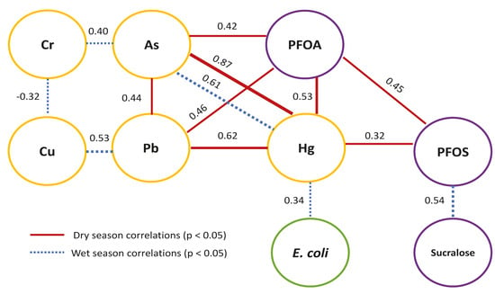
| Dry | E. coli | As | Cd | Cr | Cu | Pb | Hg | NO3− | PFOS | PFOA |
| As | −0.02 | |||||||||
| Cd | −0.02 | −0.02 | ||||||||
| Cr | −0.02 | 0.11 | 0.20 | |||||||
| Cu | −0.13 | −0.08 | 0.20 | −0.16 | ||||||
| Pb | −0.12 | 0.44 ** | −0.06 | −0.16 | 0.28 | |||||
| Hg | −0.06 | 0.87 *** | −0.06 | −0.12 | 0.01 | 0.62 *** | ||||
| NO3− | −0.17 | −0.19 | 0.06 | −0.21 | −0.23 | −0.19 | −0.20 | |||
| PFOS | 0.17 | 0.16 | −0.18 | −0.12 | −0.10 | 0.17 | 0.32 * | −0.18 | ||
| PFOA† | −0.10 | 0.42 ** | −0.10 | −0.12 | 0.04 | 0.46 ** | 0.53 ** | −0.21 | 0.45 ** | |
| Sucralose | 0.09 | −0.04 | 0.02 | −0.24 | 0.27 | −0.13 | −0.11 | −0.19 | −0.01 | −0.14 |
| Wet | E. coli | As | Cd | Cr | Cu | Pb | Hg | NO3− | PFOS | PFOA |
| As | 0.09 | |||||||||
| Cd | 0.07 | 0.10 | ||||||||
| Cr | −0.01 | 0.40 ** | −0.08 | |||||||
| Cu | −0.28 | −0.21 | −0.05 | −0.32 * | ||||||
| Pb | −0.22 | −0.10 | 0.24 | −0.21 | 0.53 *** | |||||
| Hg | 0.34 * | 0.61 *** | −0.08 | −0.09 | −0.10 | −0.07 | ||||
| NO3− | 0.18 | −0.21 | 0.26 | −0.17 | −0.27 | −0.19 | −0.14 | |||
| PFOS | −0.14 | −0.01 | 0.01 | −0.24 | 0.17 | 0.06 | −0.08 | −0.27 | ||
| Sucralose | 0.15 | −0.05 | −0.03 | −0.12 | 0.06 | −0.12 | −0.04 | −0.15 | 0.54 *** |
© 2019 by the authors. Licensee MDPI, Basel, Switzerland. This article is an open access article distributed under the terms and conditions of the Creative Commons Attribution (CC BY) license (http://creativecommons.org/licenses/by/4.0/).
Share and Cite
Ornelas Van Horne, Y.; Parks, J.; Tran, T.; Abrell, L.; Reynolds, K.A.; Beamer, P.I. Seasonal Variation of Water Quality in Unregulated Domestic Wells. Int. J. Environ. Res. Public Health 2019, 16, 1569. https://doi.org/10.3390/ijerph16091569
Ornelas Van Horne Y, Parks J, Tran T, Abrell L, Reynolds KA, Beamer PI. Seasonal Variation of Water Quality in Unregulated Domestic Wells. International Journal of Environmental Research and Public Health. 2019; 16(9):1569. https://doi.org/10.3390/ijerph16091569
Chicago/Turabian StyleOrnelas Van Horne, Yoshira, Jennifer Parks, Thien Tran, Leif Abrell, Kelly A. Reynolds, and Paloma I. Beamer. 2019. "Seasonal Variation of Water Quality in Unregulated Domestic Wells" International Journal of Environmental Research and Public Health 16, no. 9: 1569. https://doi.org/10.3390/ijerph16091569