1. Introduction
Heavy metal pollution in farmland not only destroys the normal function of the soil and hinders crop growth, but also endangers human health through the food chain [
1,
2,
3]. According to relevant statistical information, the amount of contaminated grains is up to 12 million tons in China every year [
4]. Because of the serious threat to the quality of agricultural products and the sustainable development of agriculture, accurate and rapid monitoring of heavy metal pollution has become a topic of critical importance [
5,
6].
The use of satellite remote sensing data to monitor a wide range of heavy metal pollution in farmland has become an important technical method [
7]. The current monitoring of heavy metal pollution stress in crops using remote sensing technology is based mainly on the physiological and biochemical characteristics induced by heavy metal stress and the corresponding spectral response [
8,
9,
10,
11]. For example, some experiments have revealed that heavy metal stress leads to decreases in the chlorophyll content and reflectivity in the near infrared wavelength bands, an increase in the reflectivity in the red wavelength bands, and a red edge blue-shift [
12,
13,
14]. However, the growth mechanism of crops under external stress is complex, and other environmental stress factors (e.g., pests and diseases, nutrient stress, and water stress) may have the same effect on crops [
15], resulting in similar spectral variation characteristics. These limitations are larger when identifying heavy metal stress based only on stress spectral response parameters. For instance, a sensitive method to extract heavy metal stress from multifarious environment stressors is essential for exploring the features that can truly characterize crop heavy metal stress.
Various factors may cause stress on crop growth in the complex farmland ecosystem. These environmental stress factors can be divided into volatile factors (such as pests and diseases, moisture, climate anomalies, and nutritional stress) and stable factors (such as heavy metal stress and salt stress) for crops [
16]. For a given region, stable factors persist for a certain period of time, and it is uncertain whether a volatile factor exists or not. The characteristics of heavy metal contaminants include poor migration ability, degradation resistance, and irreversibility in the soil [
17]. Thus, heavy metal stress exists during the entire crop growth cycle and has a consistent long-term influence on growth. The effect of heavy metal stress on crop growth in different years is thus similar. Other stressors are affected by diverse factors such as climate, planting habit, and management conditions [
18] with distinct interannual changes often existing in one or several growth cycles of crops. These stressors show volatility and are short-acting within the year and on interannual cycles. For example, rice stripe disease and rice planthopper damage occur in the seedling and booting stages, respectively [
19,
20]. In light of the stable interannual variation of the influence of heavy metal stress on crops, heavy metal stress can be effectively distinguished from other stressors by continuous monitoring of crops on a long time scale.
Ecophysiological changes of crops under environmental stress can be characterized by damage to a series of photosynthetic apparatuses [
21,
22]. Leaf Area Index (LAI) is a key physical quantity that characterizes the growth status of vegetation and is an indispensable parameter to describe plant photosynthesis and material energy exchange. Previous research has employed LAI to indicate the morphological and color changes of crops and to monitor the heavy metal stress of crops through the band response characteristics of visible light to shortwave infrared [
23,
24,
25,
26]. Therefore, LAI can be used as a valid indicator for monitoring the crop stress.
Currently, it is difficult to use remote sensing technology to directly estimate the LAI with long time resolution. The World Food Studies (WOFOST) model can achieve the dynamic simulation of LAI with a one-day time step through assimilating with remotely sensed information [
4,
27,
28]. When the physiological functions are at the optimal state, the crop growth curve of LAI can be simulated by potential growth level under non-stress conditions [
15]. Crops experience environment stress if suboptimal growth conditions cause their crop physiological functions to decline from their physiological standard [
29], and the amplitude of the LAI signal will be dampened once the crops suffer stress. The total stress information is hidden in the reduced amplitude, including heavy metal stress and other stress information. In consequence, the amplitude of the LAI signal on stressed rice is the subtraction of the intrinsic growth signal of the crop and total stress signal. The LAI time series can thus be considered to contain three types of information: the inherent growth tendency, persistent environmental stress (heavy metal stress), and other stressors.
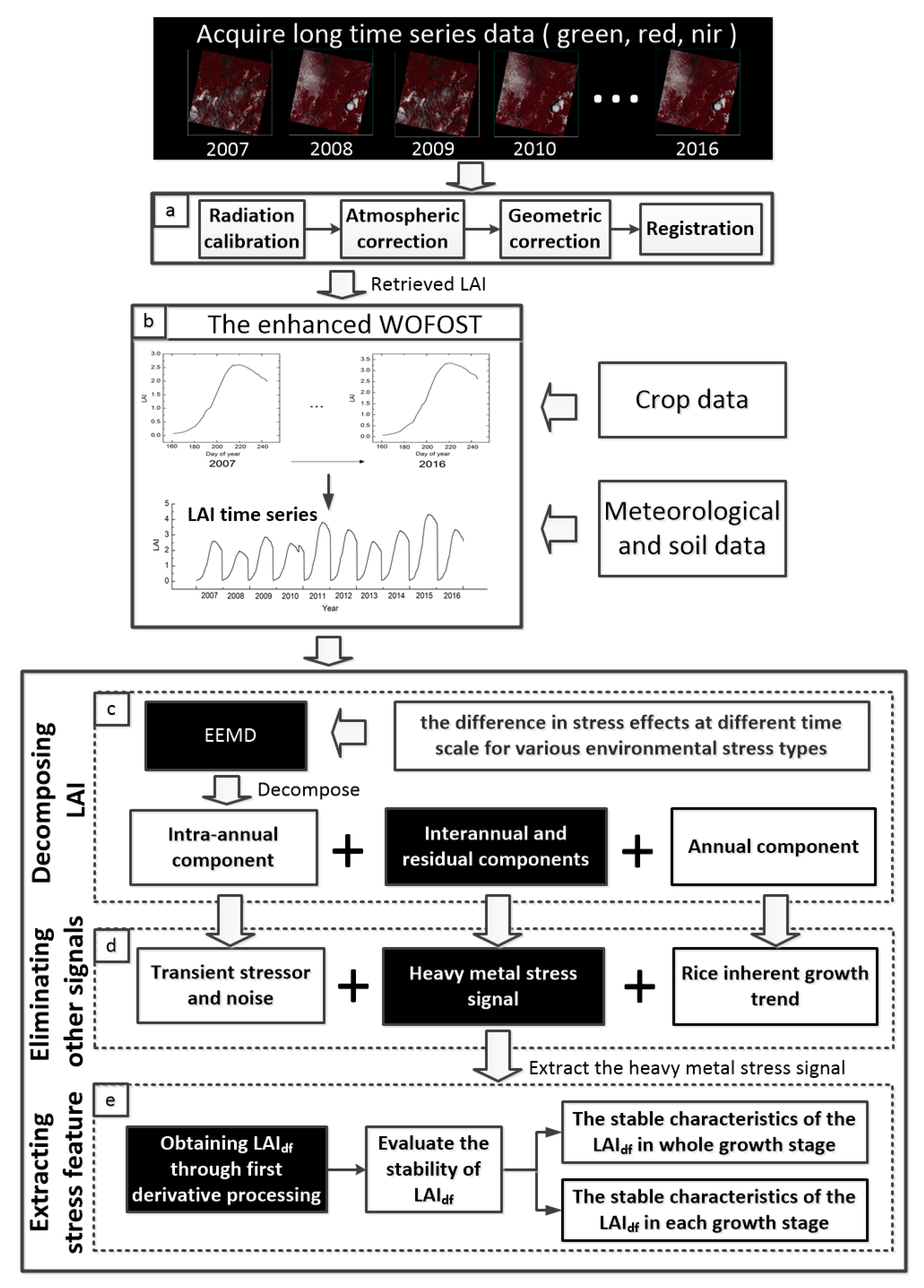
Thus, in this study, we extracted the rice heavy metal stress signal feature by using a decade of remotely sensed data. By focusing on the difference in stress effects at different time scales for various environmental stress types, the LAI time series simulated by the enhanced crop growth model (WOFOST) was decomposed to three kinds of signals through Ensemble empirical mode decomposition (EEMD). After getting rid of some other stress and crop innate growth signals, the remaining signal containing heavy metal stress information was extracted. Finally, we explored the features that can characterize the heavy metal stress accurately and evaluated its stability. These three analyses are the main objectives of this paper. This paper provides a reliable method using long time-series remote sensing data for accurate identification of heavy metal stress in crops, which could be further applied in the precise monitoring of heavy metal stress.
4. Results
4.1. Decomposition of LAI Time Series
On the basis of EEMD, the LAI time series was decomposed into three main components—intra-annual, annual, and interannual—as well as a residual. The standard deviation of the Gaussian white noise added in the EEMD (Nstd) and the number of times the noise was added (NE) were used to determine the decomposition effect. The Nstd range is 0.01–0.4; we chose increments of 0.01, 0.05, 0.1, 0.2, and 0.3 for adding NE 50 and 100 times. The experiment revealed that regardless of the number of additions when Nstd was the same, the decomposition results were similar. Therefore, we set NE to 100 times.
Because the annual trend of crop growth is essentially constant for ten years, the experiment was conducted using several prepared Nstd values according to a benchmark of the coefficient of determination (R
2) of the annual component among the ten years. The value with the highest correlation was chosen as the Nstd used in this study.
Table 4 illustrates the coefficient of determination of the annual component from year to year after setting up the different parameters. When the value of Nstd was 0.3, the average R
2 reached 0.927, and the relationship was at its closest. What’s more, the
p value was less than 0.05 and the correlation was prominent. Therefore, 0.3 was selected as the most appropriate Nstd value for our decomposition.
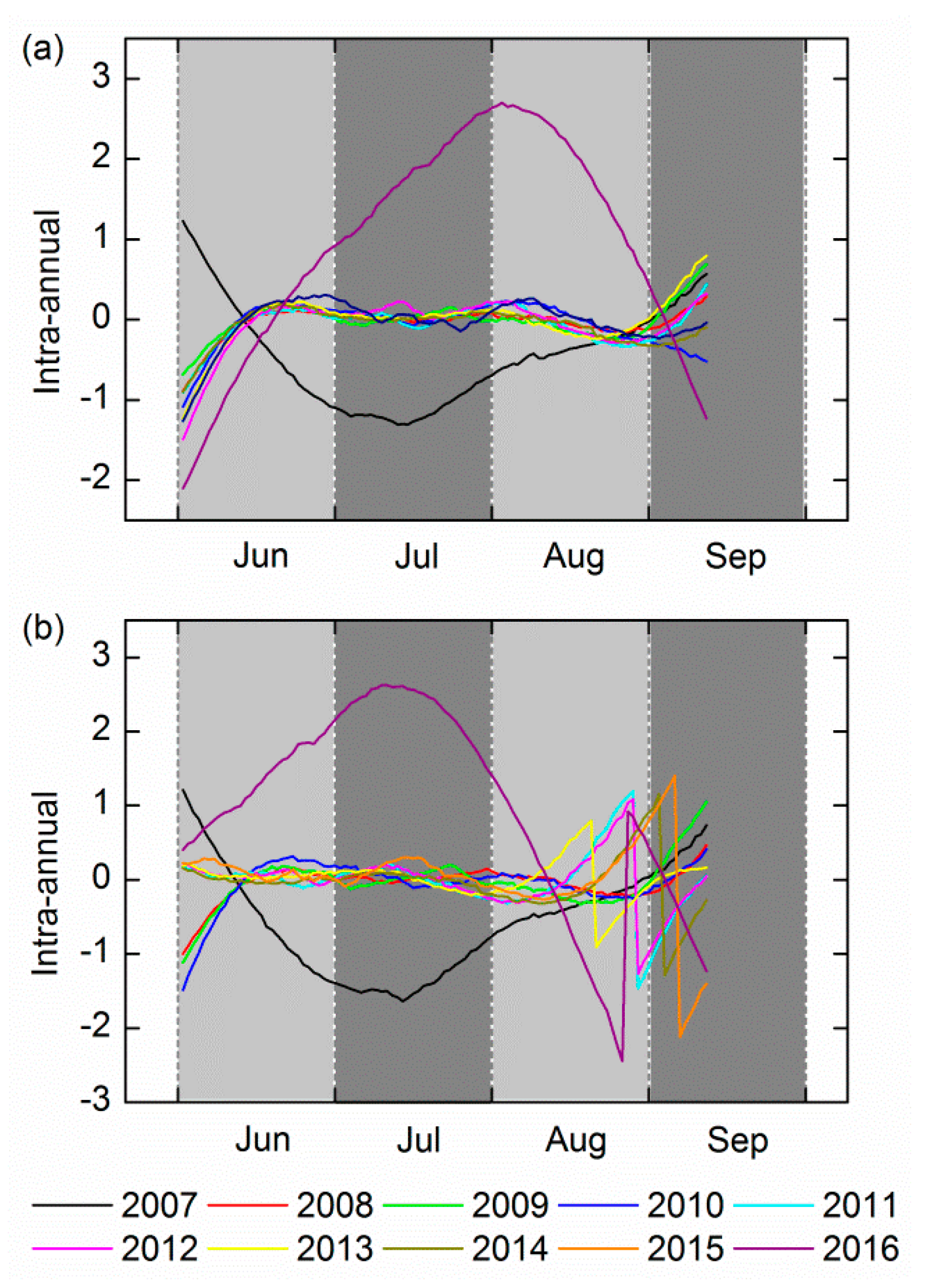
After EEMD decomposition the LAI time series produced ten (IMF1-9 and a residual) compositions, respectively. According to the analysis in the method, three kinds of signals were extracted; the signal of IMF1-4 in the LAI time series with high fluctuation frequency, the changes during the year, and interannual changes which were highly irregular. The intra-annual component is the green line in
Figure 4. The signal of IMF5 in the LAI time series is the annual component, the variation trend of which is one cycle per year (black line in
Figure 4).
The rest of the signals are the interannual component and residual (orange line in
Figure 4). In this way, the acquisition of the three kinds of signals helps us to peel off the other stress information and separate heavy metal stress signals.
4.2. Elimination of Transient Stressors and Noise
The intra-annual component for the entire growth period of the decade is shown in
Figure 5, with the exception of 2007 and 2016, the signal for 2008–2015 fluctuated frequently throughout the whole growing process.
Table 5 lists the R
2 values of the signal across the ten year period for each growth stage (June (tillering stage), July (booting stage), August (flowering stage), and September (ripening stage)). The range of average R
2 values was from 0.268 to 0.360. The lower R
2 demonstrated that they had low similarity, and thus that stability was not strong.
The noise from other environmental factors that were present can cause long-term fluctuations in the signal, so the fluctuations for the years from 2008 to 2015 may be the result of noise. Conversely in 2007 and 2015 the signal frequency is lower compared to other years, and the vibration amplitude is larger. This probably results from transient stress, such as moisture, pests, and diseases, because the impact on rice from these factors relative to the environmental factors is more obvious. The conclusions drawn from the analysis are that the intra-annual component can be proven to be unstable signals containing transient stressors and noise.
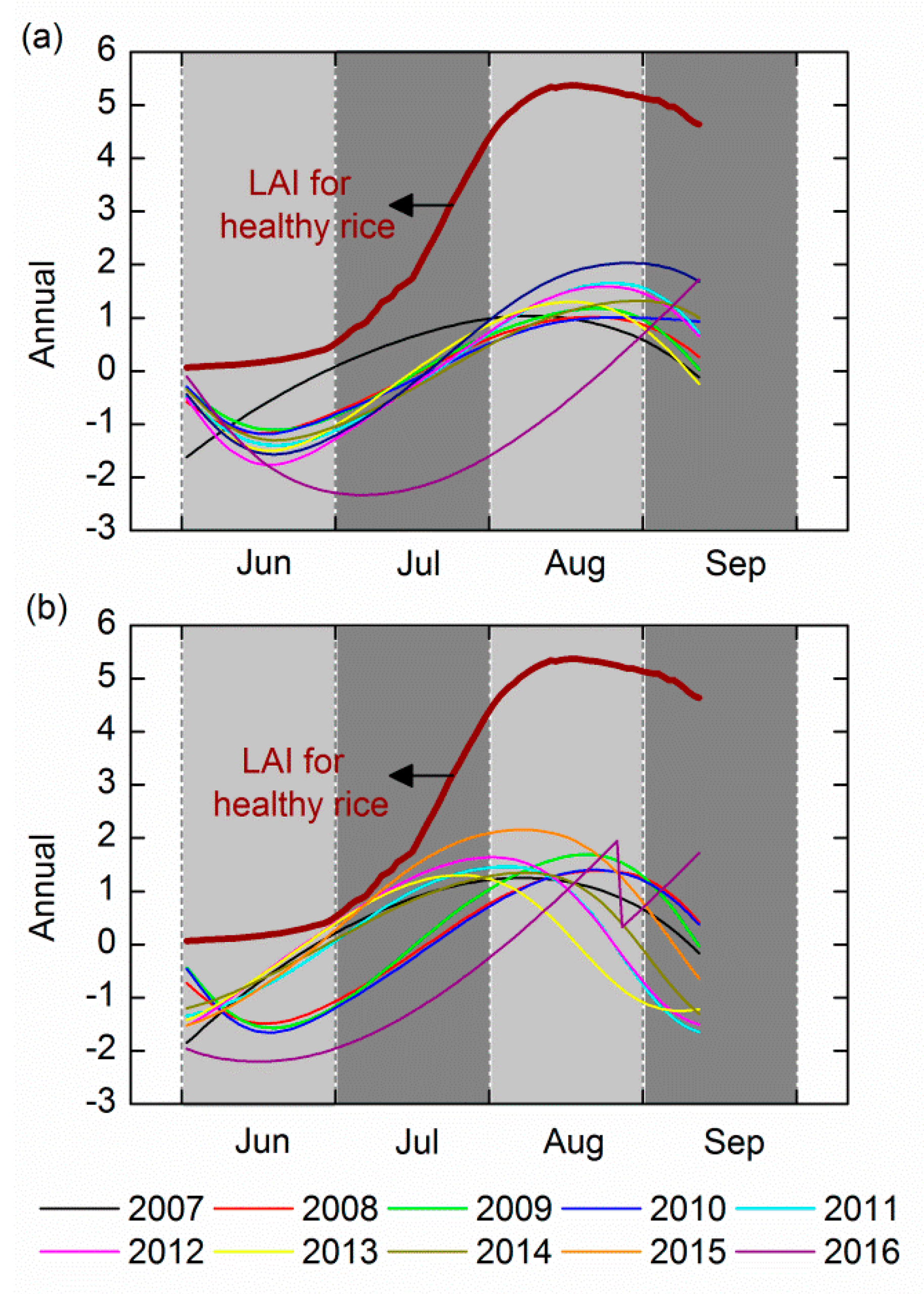
4.3. Exclusion of the Inherent Growth Trend of Rice
Figure 6 displays the contrast of the annual component and the LAI time series for healthy rice simulated with the enhanced WOFOST. In general, there were oscillations with a peak in the whole growth period, and their trajectories were characterized by similarity.
Table 6 shows the R
2 between LAI time series for healthy rice and the annual signal at both sites A and B. At site A, despite the abnormal trend in the years of 2016 and 2007, the average R
2 reached 0.853; the average R
2 at site B was 0.754 and the R
2 in 2016 is also not high enough. In general, the LAI time series on healthy rice is relatively highly correlated with the annual signal. The results verified that the annual component was able to reveal the signal response to the rice’s inherent growth trend.
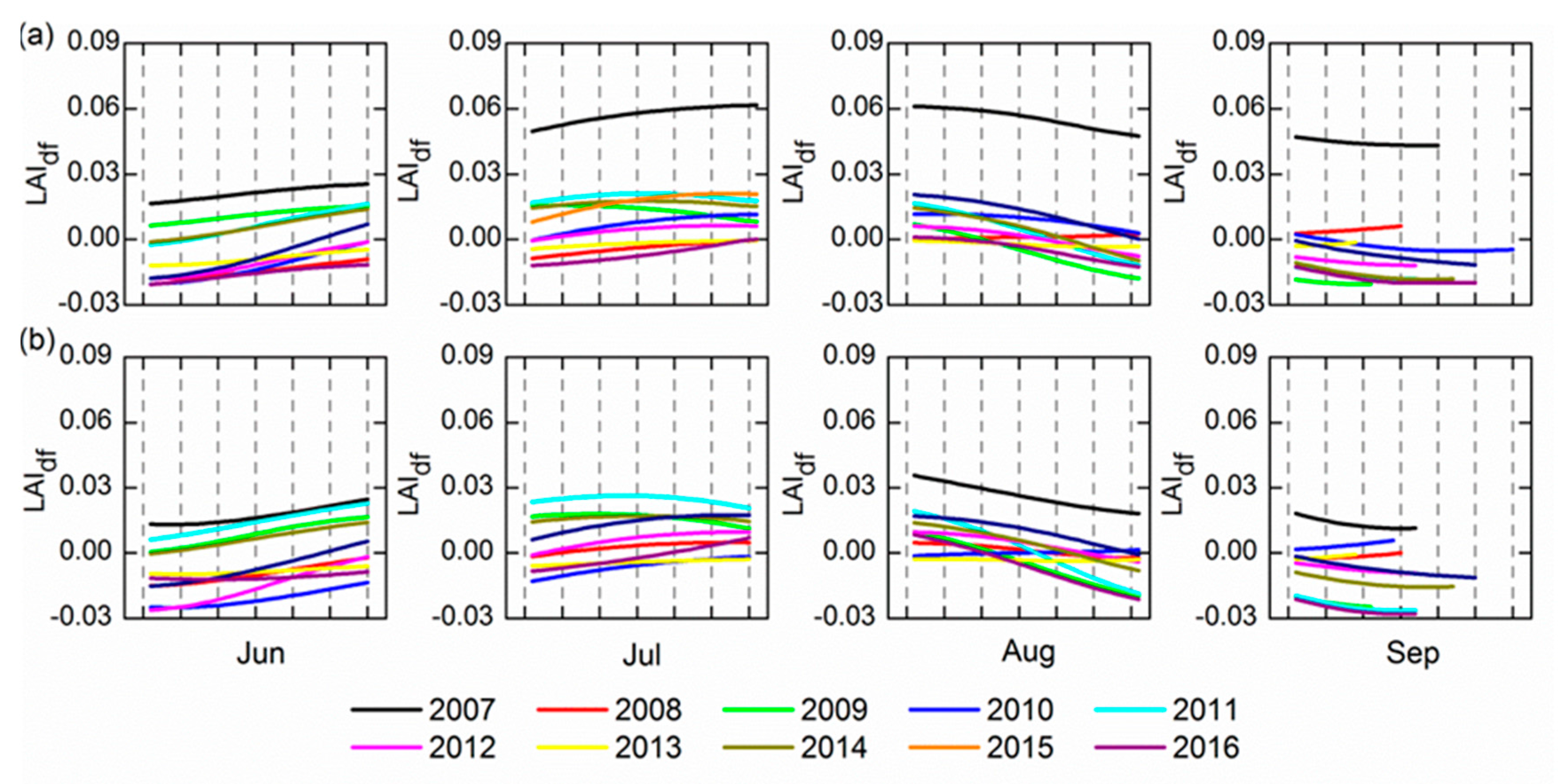
4.4. Acquisition of Stable Features of Rice Heavy Metal Stress
By eliminating the above two kinds of components, the heavy metal stress information remains in the sum of the inter-annual component and the residual (LAI
d). To further exclude the interference from other low frequency signals and extract the stable heavy metal stress feature, the LAI
df time series was obtained through the first derivative processing to LAI
d. These LAI
df were compared in the four growing periods (
Figure 7). The growing trend in June and July and the reducing trend in August and September were relatively stable during the 10 years of change. Nevertheless, in 2011 and 2014 there were abnormal change trends of LAI
df showed by both sites A and B in July.
We conducted a stability analysis from two aspects. On the one hand, the analysis of the R
2 values for the LAI
df signal in each growth period across the ten years is shown in
Table 7. We can see that the LAI
df signal has high similarity apart from in July; the similarity is at its best in June at both sites A and B and the stability is relatively strong. On the other hand, because the LAI
df sequences were close to the linear trend in the four growth periods each year, their linear fitting was used to analyze their trend discrepancy. The fitting precision in addition to some of the abnormal values were found to be relatively high by experiment, indicating that this method more reliably denotes the dynamic. The slope ratios of each line fitting equation (LAI
dfs) reflect the dynamic situation of the LAI
df.
Table 8 compares the standard error of 10-year LAI
dfs in different growth periods.
The results show the fluctuant magnitude of the LAIdfs across the 10 years. The fluctuations of the LAIdfs for the decade were both minimal in June regardless of the site. In summary, it is concluded that the stability of trend of the LAIdf was most obvious in June. It is possible that the LAIdf was less sensitive in other periods, and the stability was thus not prominent.
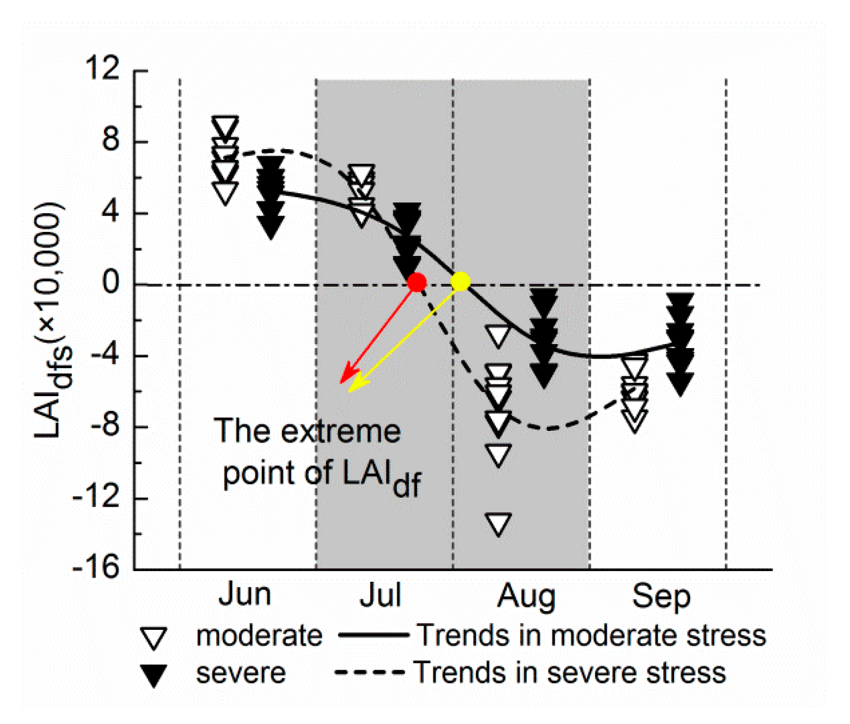
The dynamics of LAI
dfs for sites A and B over the entire growth phase are shown in
Figure 8. The LAI
dfs at site A reached the zero point in August, and site B reached zero in July. The results demonstrate that the overall dynamic of LAI
df throughout the growing season at site A was similar to that at site B: the trajectories appeared to grow first and then fall as a whole, and all showed a peak during July to August. Based on the above analysis, the LAI
df of ten years has an equivalent variation trend both in the whole growth period and in each of the growing stages. This indicates that LAI
df can be regarded as a stable feature to represent the rice heavy metal stress signal.
5. Discussion
The EEMD method for extracting the heavy metal stress signals in rice based on long time series LAI was presented. The reasonable characteristics of heavy metal stress were produced using a first derivative operation. The LAIdf had a good stability in the four growth periods and for the full growth process. This was supported by the coefficient of determination, the standard deviation statistic and trajectory analysis for LAIdf, which indicated that the EEMD is a reliable means to extract the heavy metal stress signal.
The peak of the LAI
df indicates that the change rate of LAI
d is maximal at this time only under heavy metal stress. LAI
d can be regarded as the reduced magnitude of the curve of the LAI time series in rice under heavy metal stress relative to non-stressed rice. In other words, the effect of stress on the crop growth. During the vigorous vegetative growth period, the growth center is the growth and development of vegetative organs. Studies have shown that heavy metal pollution in this period can cause serious damage to the chloroplast such as the dissolution of the membrane system of the chloroplast [
48,
49,
50,
51,
52]. Thus, the inhibitory effect on rice growth induced by heavy metal stress will get faster. Later, owing to the rapid increase in crop biomass, the heavy metal content in the crop will be subjected to a large degree of dilution, and the performance of heavy metal stress begins to weaken. Therefore, it is possible that during July to August, the maximum inhibition of photosynthesis was reached during the vigorous growth period; the change rate of the effect of heavy metal stress at this stage reached the maximum; and LAI
df also reached its maximum.
It could be argued that in contrast to the trajectory of LAI
df over the ten years, there are two years with abnormal readings in July. One reason for this is that, relative to the other three months, this period does not have a very clear stable trend. The trend in this stage also exhibits greater uncertainties. Moreover, the trend inconsistencies are most likely to result from sensor inconsistencies (e.g., orbital drift or defective corrections) or between-sensor inconsistencies (e.g., historic processing differences or differences in sun-target-sensor geometry) [
39]. The combination of multi-source sensor data has an effect on the retrieved LAI, which as the input parameter of the enhanced WOFOST; ultimately has influence on the simulation results of the LAI. Another reason may be that the LAI
df is not stable enough on the scale of the month; this can be further verified by selecting other indicators, which in the case of other conditions remain unchanged. All of these factors contribute to the broader uncertainties associated with the LAI
df. In general, even though the performance of LAI
df in July is not particularly desirable, the trend of change over the 10 years was relatively stable. The LAI
df can still be used as a stable feature to reveal the rice heavy metal stress.
This study is based on the discrepancy between the stress features at different time scales; thus, we accessed the dataset from 2007–2016. The land use type of the study area during the 10 years showed little difference and the heavy metal stress in the study area is dominant status because of the potential hazards. Therefore, the extent of crop stress by heavy metals can be regarded as a constant factor. However, the retrieved LAI was calculated from the obtained rice pixels through supervised classification in the region, which can produce some error. In addition, the LAI values of the study area were averaged at each phase, and the number of rice samples in the past decade changed, which could have also had an effect on the results. The influencing factors of the enhanced WOFOST assimilation model are weather parameters and crop parameters. Our 10 years of meteorological data were obtained from a weather station. Owing to the small range of the study area, the variation in weather conditions did not lead to uncertainty, however, it is necessary to consider the regional distribution of climate data if this method is to be applied on a large regional scale [
15]. For the EEMD decomposition model, different parameters affected the results of the decomposition, therefore, uncertainty exists in the screening process. Moreover, if the origin signal is not properly de-noised beforehand, then the noise involved in decomposition increases the number of layers of decomposition. Unnecessary decomposition layers cause error and cumulative errors, which reduces the accuracy of signal decomposition [
53]. However, the choice of different de-noising methods before the signal is input will produce effects of varying degrees for the original signal, and the results of the decomposition will also vary in performance. The LAI time series was not properly de-noised prior to decomposition in our experiment. Although these errors and uncertainties exist, it does not mean that the features we acquired from the experiment are not exact. The characteristics of the heavy metal stress signal we obtained are, to some extent, stable.
For the obtained rice heavy metal stress signal features, the stability is still insufficient. We can further explore whether other indicators can better characterize heavy metal stress based on the proposed method. We can establish a comprehensive index of some indicators to improve the stability; and more accurately assess the rice characterization results from the differences in stress levels. The determination of a comprehensive evaluation index and the establishment of an evaluation model of heavy metal stress are topics for our future research.
6. Conclusions
This study describes a new concept of extracting stable heavy metal stress features and provides a research method for accurate remote sensing identification of heavy metal stress in crops. In this paper, we used the EEMD approach to extract rice heavy metal stress signals based on multi-year remote sensing data and excavated the varying features of heavy metal stress signals. The change trends of the LAIdf that characterize the heavy metal stress in the whole growth period were similar, and were also consistent in each growth period. The stability of the LAIdf response to rice heavy metal stress can be best evaluated in June.
In summary, according to differences in temporal characteristics presented by all types of stress effects, the method of EEMD can effectively be used to identify rice heavy metal stress. The LAIdf manifests as a stable heavy metal stress feature and well embodies the desired meaning: the influence of heavy metal stress on rice growth. This study provides a scientific basis for remote sensing monitoring of crop environmental stress. The EEMD method combined with the stress mechanism, stress parameters, and stress time effects can promote the accuracy of crop heavy metal stress monitoring.


