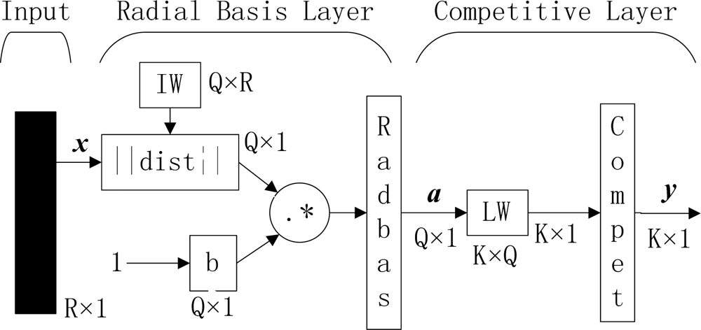
Figure 1.
Outline of PNN (R, Q, and K represent number of elements in input vector, input/target pairs, and classes of input data, respectively. IW and LW represent input weight and layer weight, respectively).
Figure 1.
Outline of PNN (R, Q, and K represent number of elements in input vector, input/target pairs, and classes of input data, respectively. IW and LW represent input weight and layer weight, respectively).
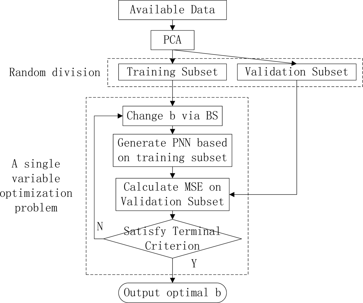
Figure 2.
The outline of our method.
Figure 2.
The outline of our method.
Figure 3.
Using normalization before PCA.
Figure 3.
Using normalization before PCA.
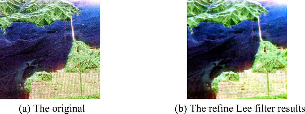
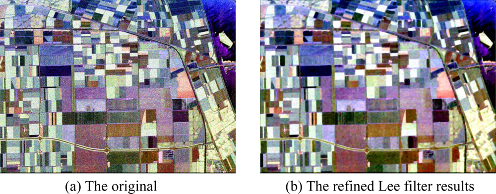
Figure 4.
Pauli image of sub-area of San Francisco.
Figure 4.
Pauli image of sub-area of San Francisco.
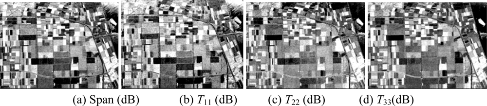
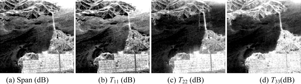
Figure 5.
Basic span image and three channels image.
Figure 5.
Basic span image and three channels image.
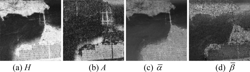
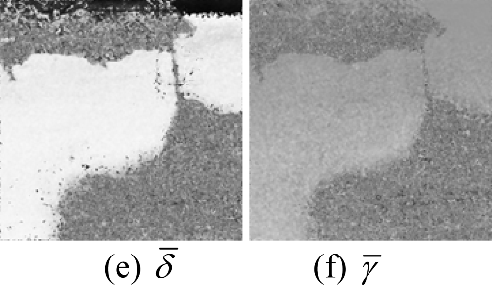
Figure 6.
Parameters of H/A/Alpha decomposition.
Figure 6.
Parameters of H/A/Alpha decomposition.
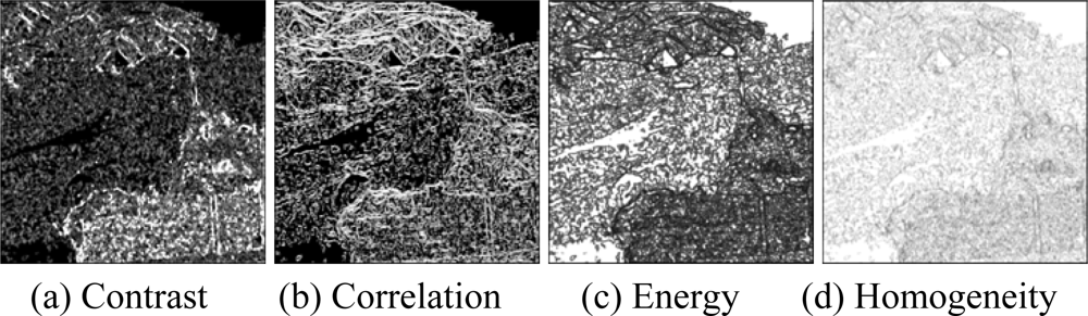
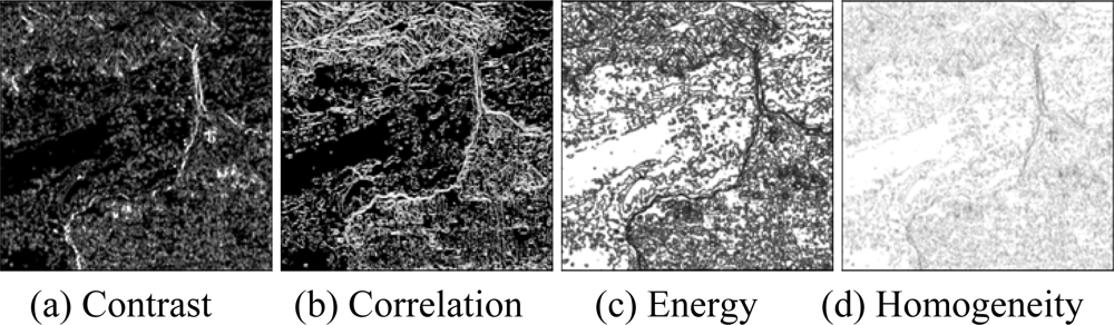
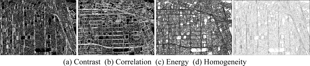
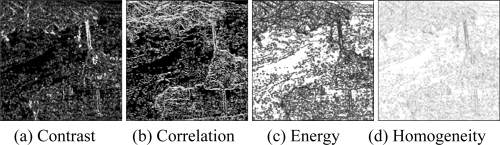
Figure 7.
GLCM-based features of T11.
Figure 7.
GLCM-based features of T11.
Figure 8.
GLCM-based features of T22.
Figure 8.
GLCM-based features of T22.
Figure 9.
GLCM-based features of T33.
Figure 9.
GLCM-based features of T33.
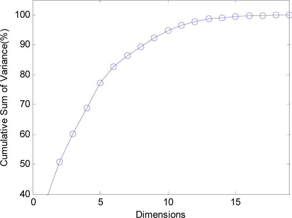
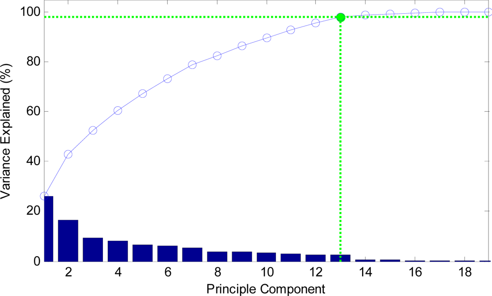
Figure 10.
The curve of cumulative sum of variance with dimensions.
Figure 10.
The curve of cumulative sum of variance with dimensions.
Figure 11.
Sample data of San Francisco (Red denotes sea, green urban areas, blue vegetated zones).
Figure 11.
Sample data of San Francisco (Red denotes sea, green urban areas, blue vegetated zones).
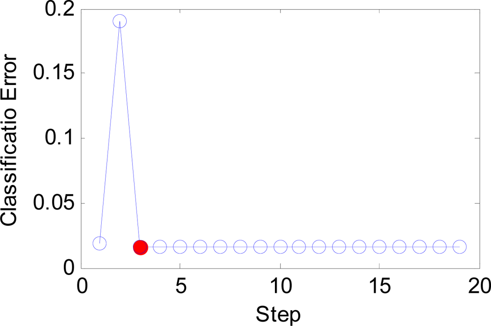
Figure 12.
The curve of error versus step.
Figure 12.
The curve of error versus step.
Figure 13.
The curve of b versus step.
Figure 13.
The curve of b versus step.
Figure 14.
Classification results of the whole image.
Figure 14.
Classification results of the whole image.
Figure 15.
Pauli Image of Flevoland (1024 × 750).
Figure 15.
Pauli Image of Flevoland (1024 × 750).
Figure 16.
Basic span image and three channels image.
Figure 16.
Basic span image and three channels image.
Figure 17.
Parameters of H/A/Alpha decomposition.
Figure 17.
Parameters of H/A/Alpha decomposition.
Figure 18.
GLCM-based features of T11.
Figure 18.
GLCM-based features of T11.
Figure 19.
GLCM-based features of T22.
Figure 19.
GLCM-based features of T22.
Figure 20.
GLCM-based features of T33.
Figure 20.
GLCM-based features of T33.
Figure 21.
The curve of cumulative sum of variance with dimensions.
Figure 21.
The curve of cumulative sum of variance with dimensions.
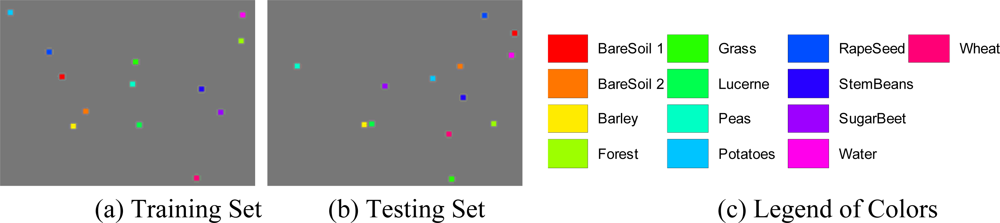
Figure 22.
Sample data areas of Flevoland.
Figure 22.
Sample data areas of Flevoland.
Figure 23.
The curve of error versus step.
Figure 23.
The curve of error versus step.
Figure 24.
The curve of b versus step.
Figure 24.
The curve of b versus step.
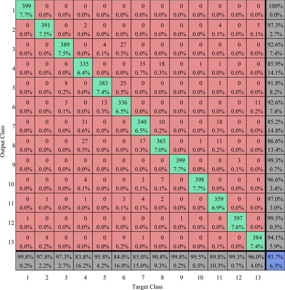
Figure 25.
Confusion matrix comparison on train area (values are given in percent) The overall accuracy is 93.71%.
Figure 25.
Confusion matrix comparison on train area (values are given in percent) The overall accuracy is 93.71%.
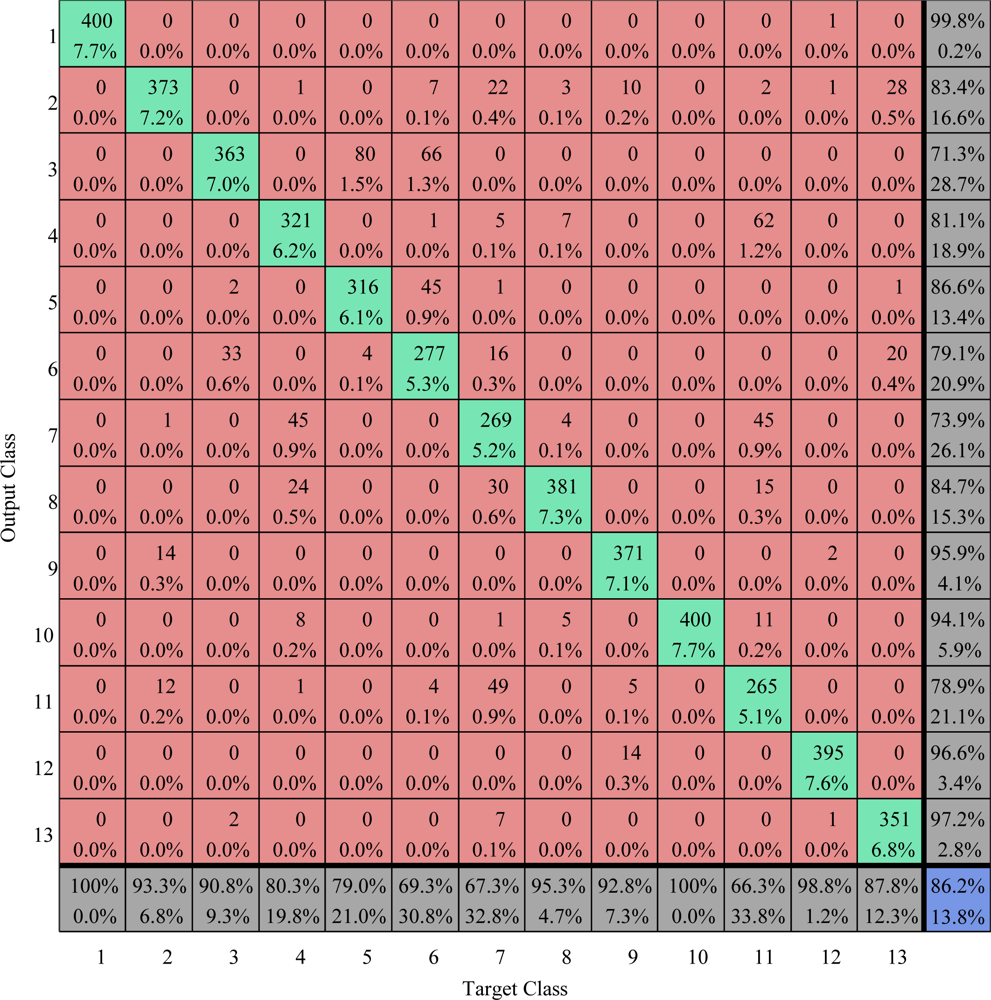
Figure 26.
Confusion matrix comparison on test area (values are given in percent) The overall vccuracy is 86.2%.
Figure 26.
Confusion matrix comparison on test area (values are given in percent) The overall vccuracy is 86.2%.
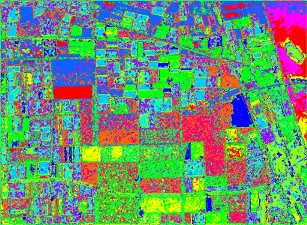
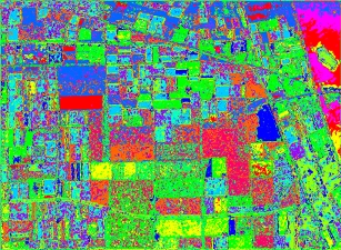
Figure 27.
Classification Map of our method.
Figure 27.
Classification Map of our method.
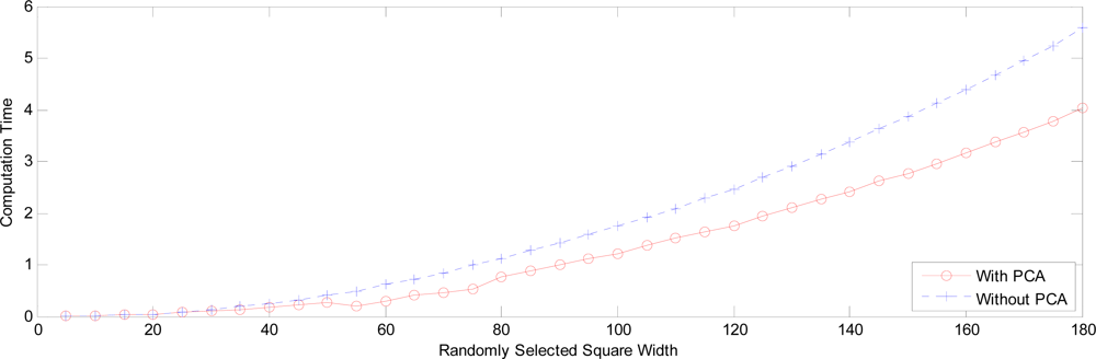
Figure 28.
Computation time with square width.
Figure 28.
Computation time with square width.
Figure 29.
The overall accuracy versus square width.
Figure 29.
The overall accuracy versus square width.
Table 1.
Pauli bases and their corresponding meanings.
Table 1.
Pauli bases and their corresponding meanings.
| Pauli Bases | Meaning |
|---|
| Sa | Single- or odd-bounce scattering |
| Sb | Double- or even-bounce scattering |
| Sc | Those scatterers which are able to return the orthogonal polarization to the one of the incident wave (forest canopy) |
Table 2.
Properties of GLCM.
Table 2.
Properties of GLCM.
| Property | Description | Formula |
|---|
| Contrast | Intensity contrast between a pixel and its neighbor | |
| Correlation | Correlation between a pixel and its neighbor (μ denotes the expected value, and σ the standard variance) | |
| Energy | Energy of the whole image | |
| Homogeneity | Closeness of the distribution of GLCM to the diagonal | |
Table 3.
Detailed data of PCA on 19 features.
Table 3.
Detailed data of PCA on 19 features.
| Dimensions | 1 | 2 | 3 | 4 | 5 | 6 | 7 | 8 | 9 |
| Variance (%) | 37.97 | 50.81 | 60.21 | 68.78 | 77.28 | 82.75 | 86.27 | 89.30 | 92.27 |
|
| Dimensions | 10 | 11 | 12 | 13 | 14 | 15 | 16 | 17 | 18 |
| Variance (%) | 94.63 | 96.36 | 97.81 | 98.60 | 99.02 | 99.37 | 99.62 | 99.80 | 99.92 |
Table 4.
Comparison of confusion matrix. (O denotes the output class, T denotes the target class).
Table 4.
Comparison of confusion matrix. (O denotes the output class, T denotes the target class).
| Training Area | Testing Area |
|---|
| Sea(T) | Urb(T) | Veg(T) | Sea(T) | Urb(T) | Veg(T) |
|---|
|
|---|
| 3-layer BPNN | Sea(O) | 7158 | 4 | 60 | 3600 | 42 | 5 |
| 33.1% | 0.0% | 0.3% | 33.3% | 0.4% | 0.0% |
| Urb(O) | 0 | 6882 | 136 | 0 | 3429 | 355 |
| 0% | 31.9% | 0.6% | 0.0% | 31.7% | 3.3% |
| Veg(O) | 42 | 314 | 7004 | 0 | 129 | 3240 |
| 0.2% | 1.4% | 32.4% | 0.0% | 1.2% | 30.0% |
|
| Our Method | Sea(O) | 7150 | 0 | 76 | 3597 | 33 | 0 |
| 33.1% | 0.0% | 0.4% | 33.3% | 0.3% | 0.0% |
| Urb(O) | 2 | 7074 | 74 | 0 | 3445 | 354 |
| 0% | 32.8% | 0.3% | 0.0% | 31.9% | 3.3% |
| Veg(O) | 48 | 126 | 7050 | 3 | 122 | 3246 |
| 0.2% | 0.6% | 32.6% | 0.0% | 1.1% | 30.1% |
Table 5.
Overall accuracies (values are given in percent).
Table 5.
Overall accuracies (values are given in percent).
| Training Area | Testing Area |
|---|
| 3-layer BPNN | 97.4% | 95.1% |
| Our Method | 98.5% | 95.3% |
Table 6.
Detailed data of PCA on 19 features.
Table 6.
Detailed data of PCA on 19 features.
| Dimensions | 1 | 2 | 3 | 4 | 5 | 6 | 7 | 8 | 9 |
| Variance (%) | 26.31 | 42.98 | 52.38 | 60.50 | 67.28 | 73.27 | 78.74 | 82.61 | 86.25 |
|
| Dimensions | 10 | 11 | 12 | 13 | 14 | 15 | 16 | 17 | 18 |
| Variance (%) | 89.52 | 92.72 | 95.50 | 98.06 | 98.79 | 99.24 | 99.63 | 99.94 | 99.97 |
Table 7.
Comparison of PNNs using polarimetric feature set, texture feature set, and combined feature set (TR denotes Classification Accuracy of Total Random).
Table 7.
Comparison of PNNs using polarimetric feature set, texture feature set, and combined feature set (TR denotes Classification Accuracy of Total Random).
| Site | Polarimetric feature set | Texture feature set | Combined feature set |
|---|
| San Francisco (TR=33.3%) | Training Area | 97.1% | 59.9% | 98.5% |
| Test Area | 87.4% | 45.9% | 95.3% |
| Flevoland (TR=7.69%) | Training Area | 92.2% | 48.0% | 93.7% |
| Test Area | 72.2% | 24.1% | 86.2% |
Table 8.
Comparison of PNN with and without our weights/biases setting (RD denotes Random Division).
Table 8.
Comparison of PNN with and without our weights/biases setting (RD denotes Random Division).
| Area Size | Computation Time | Overall Accuracy |
|---|
| Without RD | With RD | Ratio | Without RD | With RD |
|---|
| 10 × 10 | 1.0818 | 0.0231 | 46.8 | 94.8% | 94.9% |
| 20 × 20 | 4.0803 | 0.0386 | 105.7 | 95.5% | 95.5% |
| 30 × 30 | 22.4270 | 0.0751 | 298.6 | 96.3% | 96.2% |
| 40 × 40 | 58.1409 | 0.1125 | 516.8 | 95.9% | 95.4% |


