A Real-Time Smart Sensor for High-Resolution Frequency Estimation in Power Systems


 ,
,  and
and
Abstract
:1. Introduction
2. Theoretical Background
2.1. Chirp-Z Transform
2.2. Power Spectrum Analysis
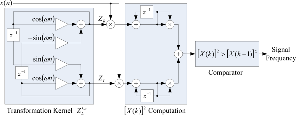
2.3. CZT Computation Unit
2.4 Computational Complexity Comparison between CZT, FFT, and Zoom-FFT
3. Simulation Results
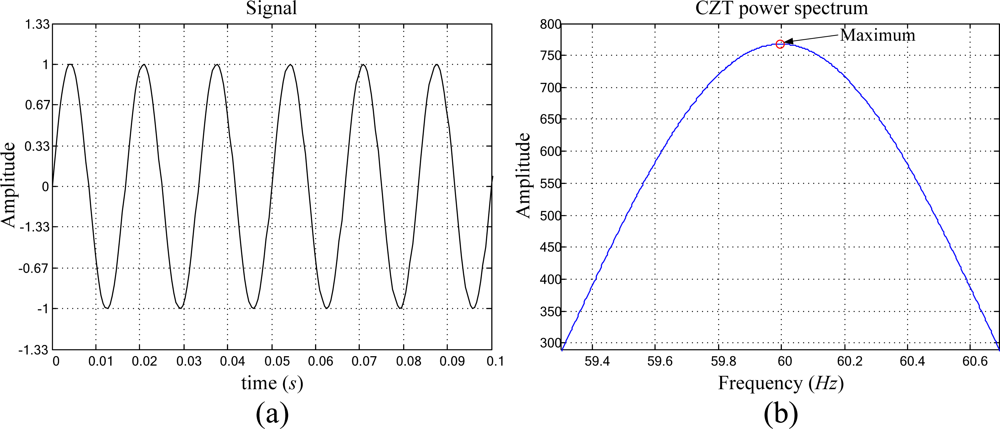
3.1. Pure periodic signal
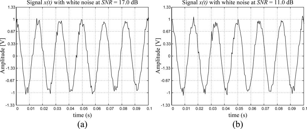
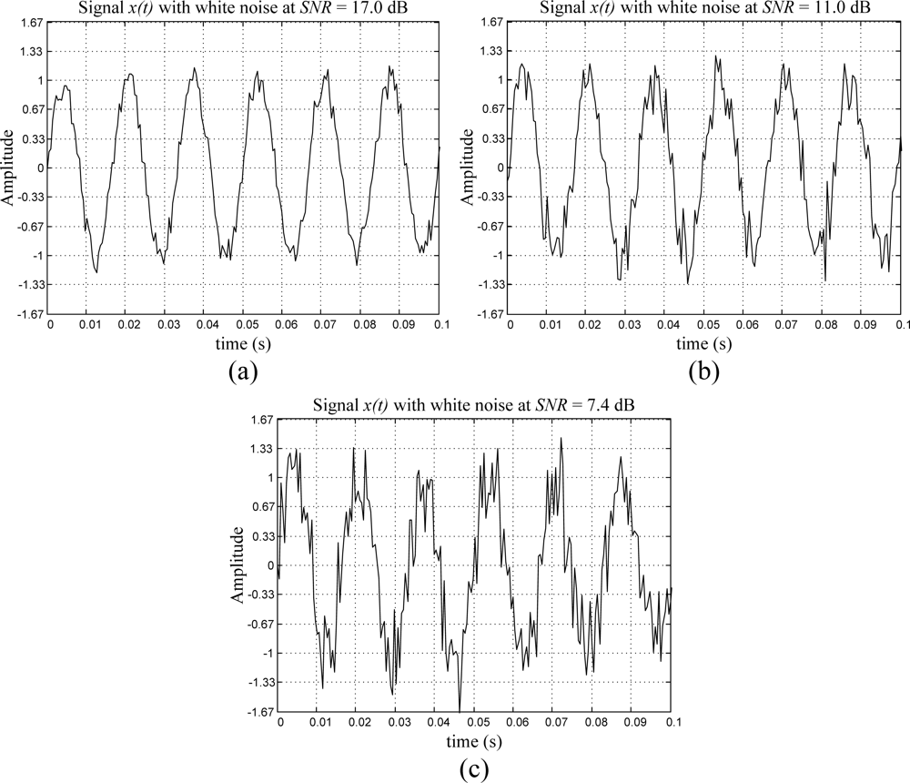
3.2. Periodic Signal with White-Noise Contamination
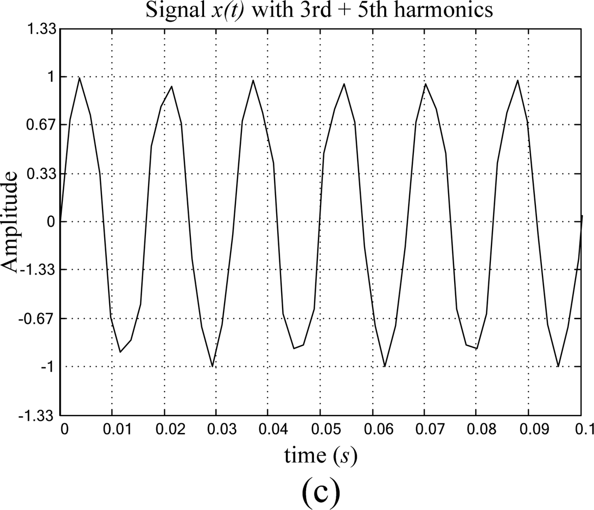
3.3. Periodic Signal plus Harmonic Contamination
3.4. Periodic Signal plus White Noise and Harmonic Contamination
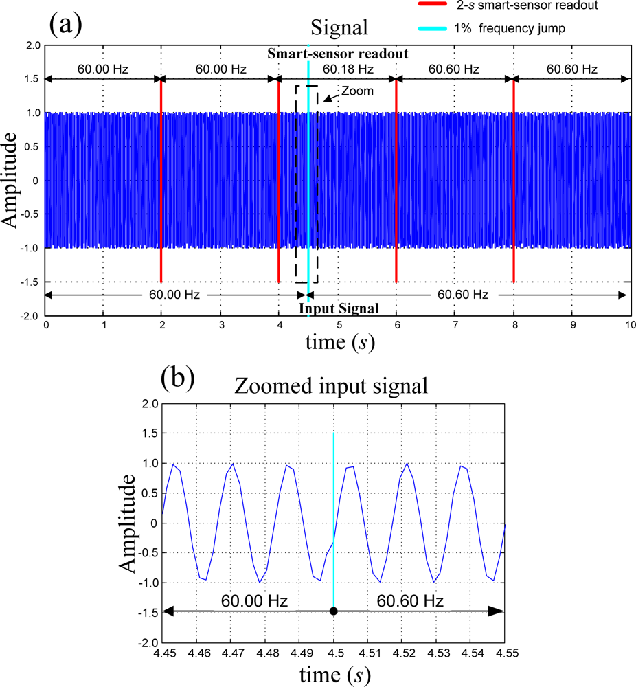
3.5. Simulation of an Instantaneous Jump on the Power Line Frequency
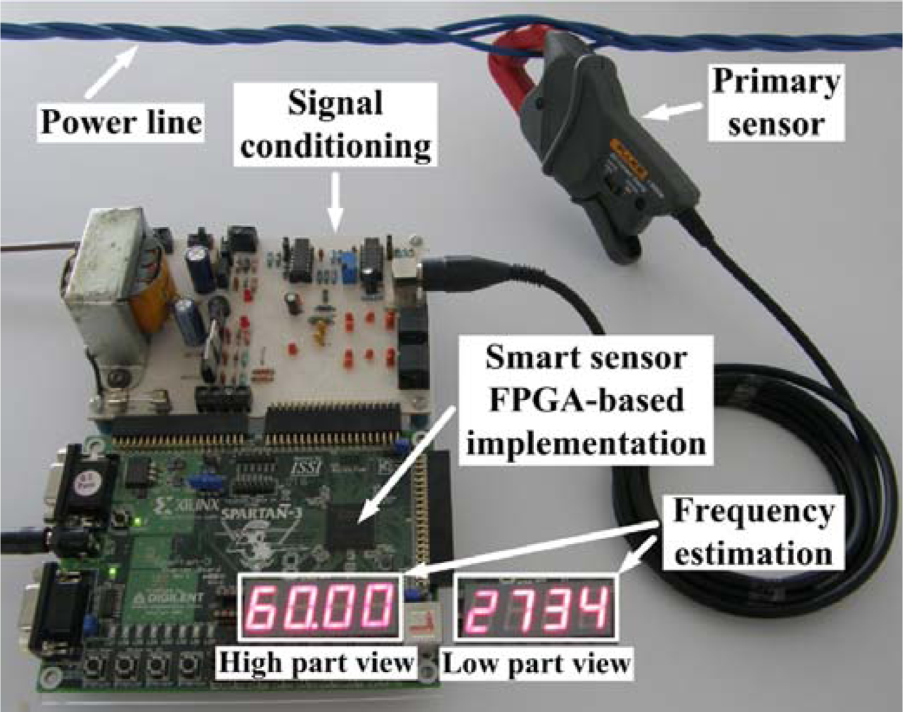
4. Experimental Results
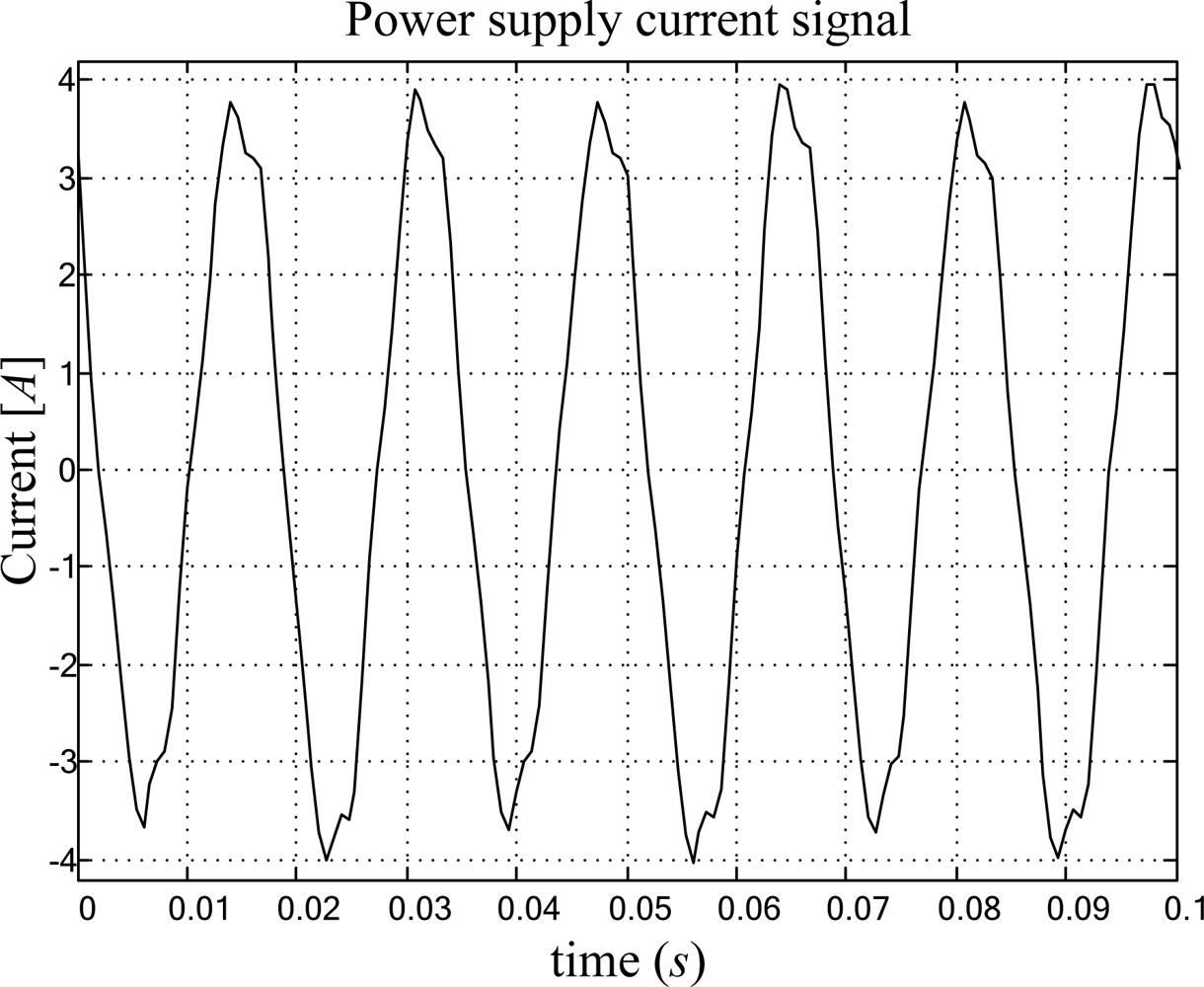
4.1. Power Supply Frequency Measurement
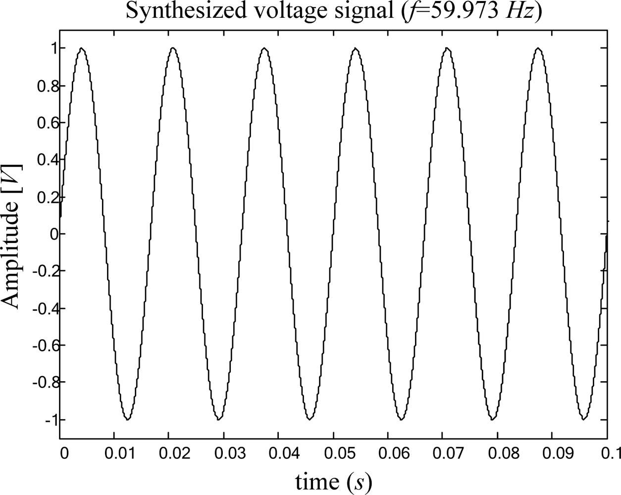
4.2. Frequency Estimation of Digitally Synthesized Functions
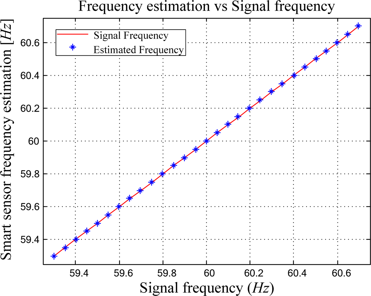
4.3. Smart Sensor Linearity
5. Discussion
6. Conclusions
Acknowledgments
References and Notes
- Xue, S.Y.; Yang, S.X. Power system frequency estimation using supervised Gauss-Newton Algorith. Measurement 2009, 42, 28–37. [Google Scholar]
- CEI/IEC 61000-4-30 International Standard. Testing and Measurement Techniques Power Quality Measurement Methods, 1st ed; International Electrotechnical Commission: Geneva, Switzerland, 2003. [Google Scholar]
- Agilent Technology. Making High-Resolution Frequency Measurements with Agilent InfiniiVision Oscilloscopes; Agilent Technologies, Inc: Santa Clara, CA, USA, April 2008. [Google Scholar]
- Venkataramanan, R.; Prabhu, K.M.M. Estimation of frequency offset using warped discrete-Fourier transform. Signal Proc 2006, 86, 250–256. [Google Scholar]
- Ohbong, K.; Taylor, F. Multi-tone detection using the warped discrete Fourier transform. Proceedings of the IEEE MWSCAS, Knoxville, TN, USA, August 2008; pp. 281–284.
- Yang, X.; Cui, X.W.; Lu, M.Q.; Fen, Z.M. Carrier recovery using FFT and Kalman filter. Proceedings of the IEEE ISPA, Aizu, Japan, July 2003; pp. 1094–1096.
- Goohyun, P.; Dongkyu, H.; Daesik, H.; Changeopon, K. A new maximum Doppler frequency estimation algorithm in frequency domain. Proceedings of the IEEE ICCS, Amsterdam, The Netherlands, April 2002; pp. 548–552.
- Chen, Y.; Fang, C. A new method of frequency measurement of power supply. Proceedings of the IEEE ICIEA, Harbin, China, May 2007; pp. 2522–2525.
- Xu, Q.Q.; Jia, S.N.; Ge, Y.-Z. Real-time measurement of mean frequency in two-machine system during power swings. IEEE T. Power Deliver 2004, 19, 1018–1023. [Google Scholar]
- López, A.; Montaño, J.C.; Castilla, M.; Gutiérrez, J.; Borrás, M.D.; Bravo, J.C. Power system frequency measurement under nonstationary situations. IEEE T. Power Deliver 2008, 23, 562–567. [Google Scholar]
- Bellini, A.; Yazidi, A.; Filippetti, F.; Rossi, C.; Capolino, G.A. High frequency resolution techniques for rotor faults detection of induction machines. IEEE T. Ind. Electron 2008, 55, 4200–4209. [Google Scholar]
- Ge, F.X.; Shen, D.X.; Sui, A.F.; Li, V.O.K. Iterative CZT-based frequency offset estimation for frequency-selective channels. Proceedings of the IEEE ICC, Seoul, Korea, May 2005; pp. 2157–2161.
- Nguyen, T.T.; Li, X.J. Application of a z-transform signal model and median filtering for power system frequency and phasor measurements. IET Gener. Transm. Distrib 2007, 1, 72–79. [Google Scholar]
- Rivera, J.; Herrera, G.; Chacon, M.; Acosta, P.; Carrillo, M. Improved progressive polynomial algorithm for self-adjustment and optimal response in intelligent sensors. Sensors 2008, 8, 7410–7427. [Google Scholar]
- Frank, R. Understanding Smart Sensors; Artech House: Norwood, MA, USA, 2000. [Google Scholar]
- Samir, M. Further structural intelligence for sensors cluster technology in manufacturing. Sensors 2006, 6, 557–577. [Google Scholar]
- Proakis, J.G.; Manolakis, D.K. Digital signal processing, Principles, Algorithms and Applications, 4th ed; Prentice-Hall: Englewood Cliffs, NJ, USA, 2006. [Google Scholar]
- Porat, B. A Course on Digital Signal Processing; John Wiley & Sons: Hoboken, NJ, USA, 1996. [Google Scholar]
- Function Generator–DS345 Function/Arbitrary Waveform Generator; Stanford Research Systems, Inc: Sunnyvale, CA, USA, 2003.
- Spartan-3 Starter Kit Board User Guide; Version 1.1; Xilinx Inc: San Jose, CA, USA, 2005.
- Texas Instruments Data Sheet ADS7841; Texas Instruments Inc: Dallas, TX, USA, 2005.
- Sadinezhand, I.; Joorabian, M. A novel frequency tracking method based on complex adaptive linear neural network state vector in power systems. Electr. Pow. Syst. Res 2009, 79, 1216–1225. [Google Scholar]
- Fan, D.; Centeno, V. Phasor-based synchronized frequency measurement in power systems. IEEE T. Power Deliver 2007, 22, 2010–2016. [Google Scholar]


| Parameter | FFT | Zoom-FFT | CZT |
|---|---|---|---|
| N | 65,536 | 65,536 | 512 |
| L | -- | 512 | 512 |
| Op | 1,048,576 | 655,360 | 262,144 |
| Tacq (s) | 100 | 100 | 1 |
| Signal + white noise at SNR (dB) | Frequency estimation (Hz) | Error (Hz) | ||
|---|---|---|---|---|
| Mean (μ) | Standard deviation (σ) | Mean (μ) | Standard deviation (σ) | |
| 17.0 | 59.9997 | 0.0040 | 0.0003 | 0.0040 |
| 11.0 | 59.9992 | 0.0066 | 0.0008 | 0.0066 |
| 7.4 | 60.0007 | 0.0106 | 0.0007 | 0.0106 |
| Signal + harmonic | Frequency estimation (Hz) | Error (Hz) | ||
|---|---|---|---|---|
| Mean (μ) | Standard deviation (σ) | Mean (μ) | Standard deviation (σ) | |
| 2nd | 60.0000 | 0.0000 | 0.0000 | 0.0000 |
| 3rd | 60.0000 | 0.0000 | 0.0000 | 0.0000 |
| 3rd + 5th | 60.0000 | 0.0000 | 0.0000 | 0.0000 |
| Signal + white noise and harmonic | Frequency estimation (Hz) | Error (Hz) | ||
|---|---|---|---|---|
| Mean (μ) | Standard deviation (σ) | Mean (μ) | Standard deviation (σ) | |
| 2nd | 60.0002 | 0.0042 | 0.0002 | 0.0042 |
| 3rd | 59.9996 | 0.0032 | 0.0004 | 0.0032 |
| 3rd + 5th | 59.9999 | 0.0038 | 0.0001 | 0.0038 |
| Signal + white noise at SNR (dB) | Frequency estimation (Hz) | Error (Hz) | ||
|---|---|---|---|---|
| Mean (μ) | Standard deviation (σ) | Mean (μ) | Standard deviation (σ) | |
| 17.0 | 60.0007 | 0.0034 | 0.0007 | 0.0034 |
| 11.0 | 60.0001 | 0.0064 | 0.0001 | 0.0064 |
| 7.4 | 60.0020 | 0.0091 | 0.0020 | 0.0091 |
© 2009 by the authors; licensee MDPI, Basel, Switzerland This article is an open access article distributed under the terms and conditions of the Creative Commons Attribution license (http://creativecommons.org/licenses/by/3.0/).
Share and Cite
Granados-Lieberman, D.; Romero-Troncoso, R.J.; Cabal-Yepez, E.; Osornio-Rios, R.A.; Franco-Gasca, L.A. A Real-Time Smart Sensor for High-Resolution Frequency Estimation in Power Systems. Sensors 2009, 9, 7412-7429. https://doi.org/10.3390/s90907412
Granados-Lieberman D, Romero-Troncoso RJ, Cabal-Yepez E, Osornio-Rios RA, Franco-Gasca LA. A Real-Time Smart Sensor for High-Resolution Frequency Estimation in Power Systems. Sensors. 2009; 9(9):7412-7429. https://doi.org/10.3390/s90907412
Chicago/Turabian StyleGranados-Lieberman, David, Rene J. Romero-Troncoso, Eduardo Cabal-Yepez, Roque A. Osornio-Rios, and Luis A. Franco-Gasca. 2009. "A Real-Time Smart Sensor for High-Resolution Frequency Estimation in Power Systems" Sensors 9, no. 9: 7412-7429. https://doi.org/10.3390/s90907412