Game and Balance Multicast Architecture Algorithms for Sensor Grid

Abstract
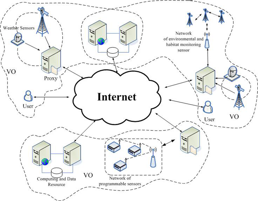
:1. Introduction
1.1. The Overview of Previous Algorithms
1.2. Motivation
Synthetically considering the space factor and the data factor
The specific implementation of the algorithms
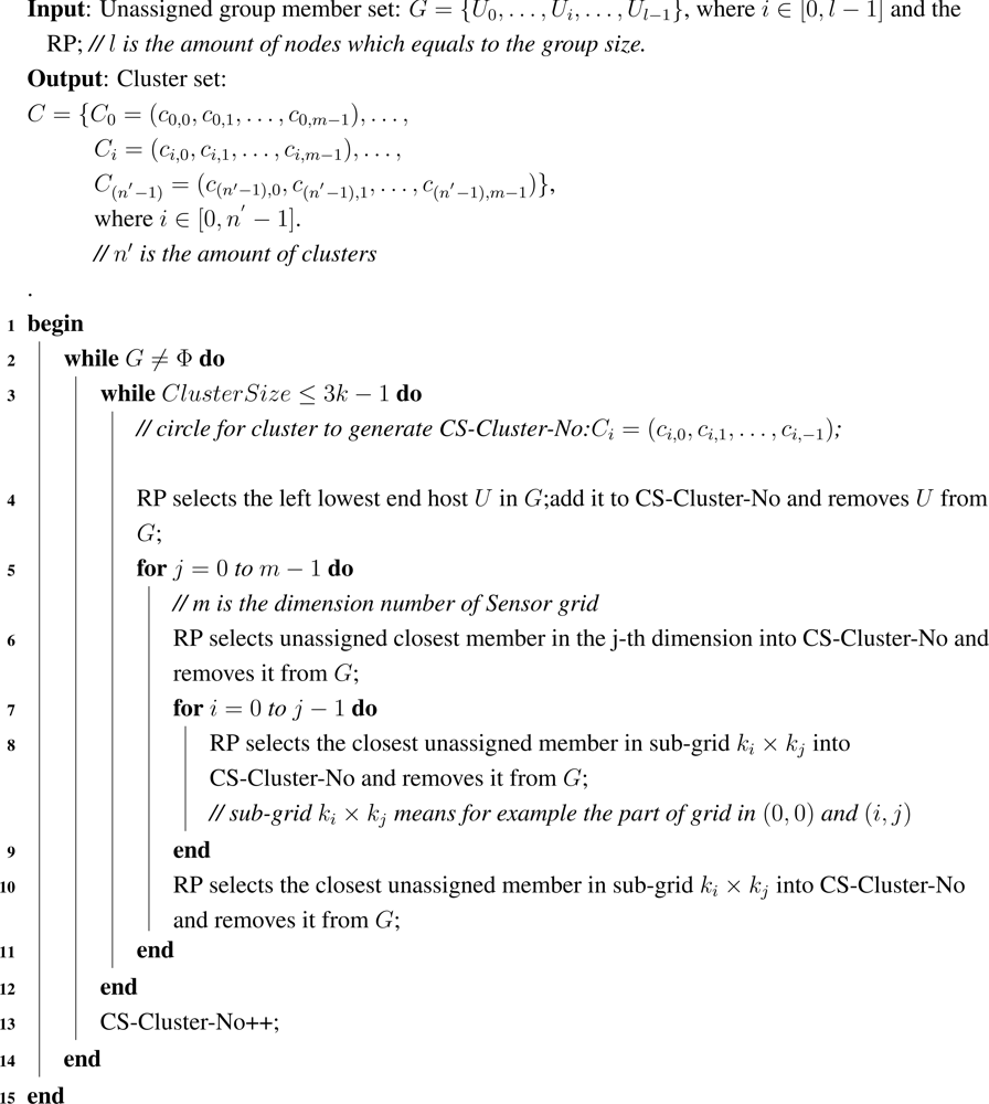
- Cluster formation algorithm that divides the group members into different clusters in terms of static delay distance;
- Relative weight vectors generation algorithm that seeks the spatial central node in every cluster, calculates the space weight of every node, searches the weight of data quantity of every node, and finds the maximum;
- The least weighted path tree algorithm that, after obtaining the space weight vector and the data quantity weight vector, builds binary simple equations, seeks linear parameters, determines the new weight vector according to the algebra sum of the two known vectors, and generates the least weighted path tree;
- Multicast routing algorithm that efficiently dispatches the multicast packets in the group on the basis of the architecture constructed by the above three algorithms.
1.3. Organization
2. The Architecture of the Algorithms for Each Weight Vector
2.1. The Space Weight Vector
2.2. The Data Weight Vector
2.3. The General Weight Vector
3. Algorithms for Game and Balance Multicast Architecture
3.1. Cluster Formation Algorithm

3.2. Relative Weight Vectors Generation Algorithm
A. To find the space center nodes as the space core Ci,a in every cluster C′i
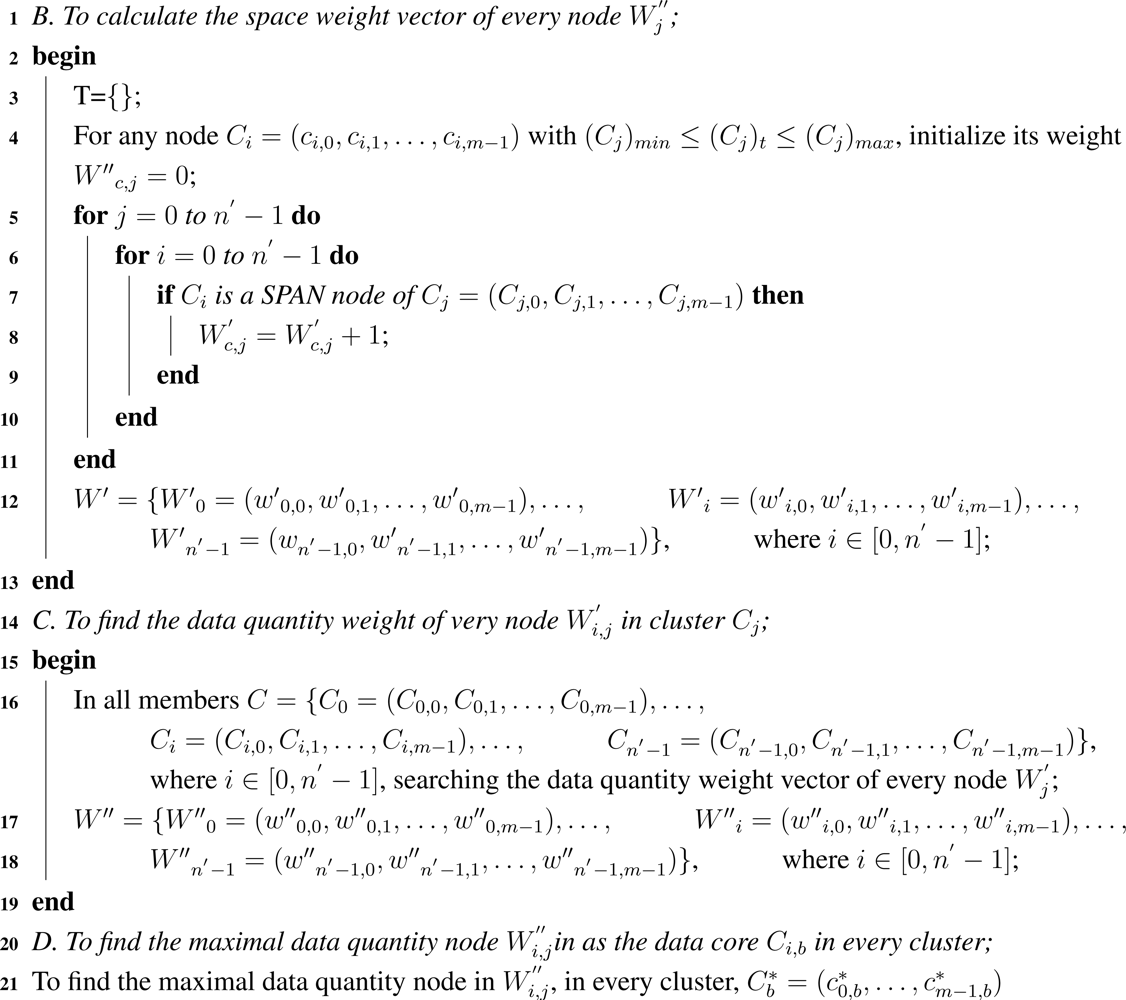
B. To calculate the space weight vector of every node W′i,j
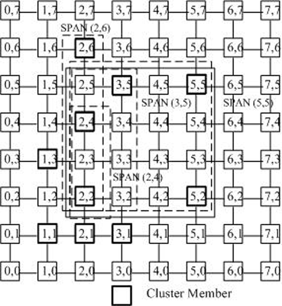
- Shortest path area nodes (SPAN): For any two nodes (x0, y0) and (x1, y1), let Xmin = min{x0, x1}, Xmax = max{x0, x1}, Ymin = min{y0, y1} and Ymax = max{y0, y1}. They uniquely define a rectangle area [x0, y0] × [x1, y1]. Each node (x, y) in [x0, y0] × [x1, y1], which is on one of the shortest paths between (x0, y0) and (x1, y1), so it is called the shortest path area nodes (SPAN) between (x0, y0) and (x1, y1).
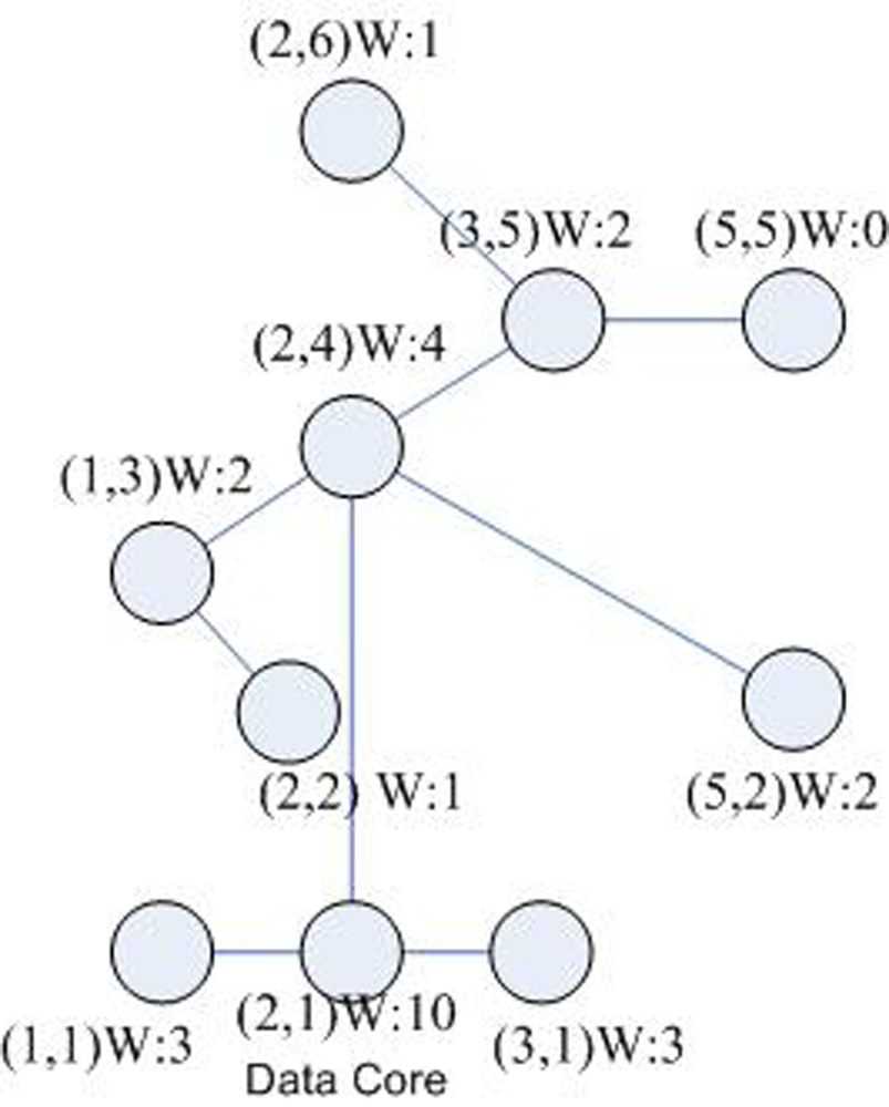
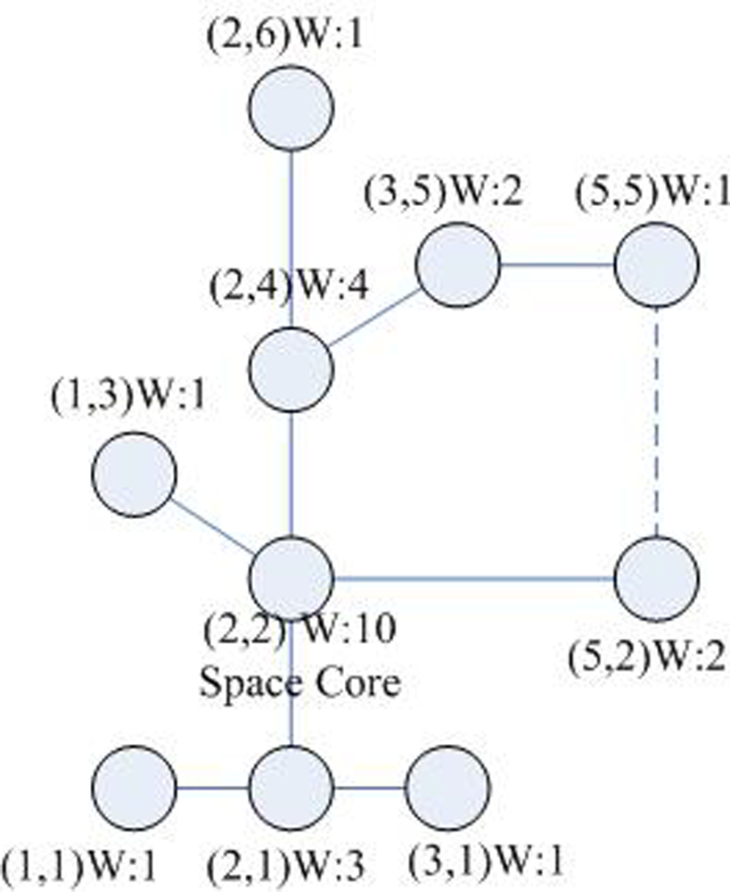
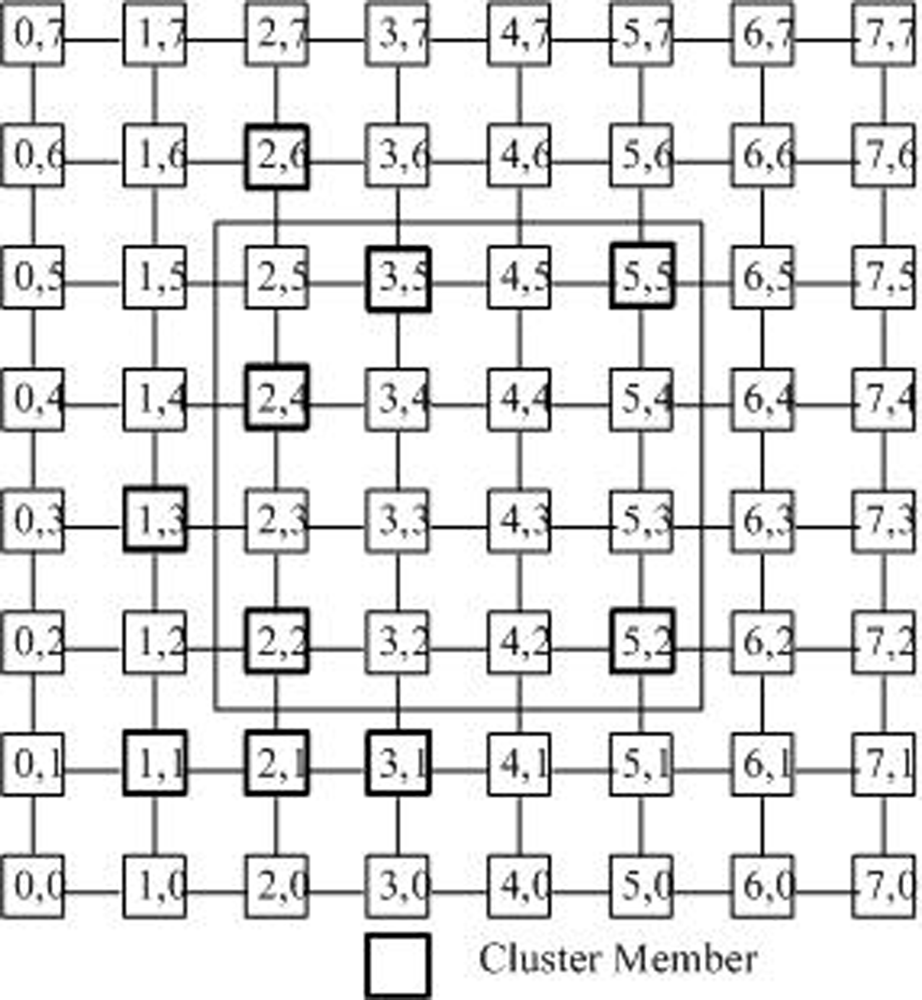
- SPAN nodes of a cluster member: When the tree is built in the cluster with the size of n, all nodes Cj(xj, yj) in the SPAN area [x0, y0] × [xi, yi] from the core (i.e., the root of the tree)c*(x*, y*) to a cluster member ci(xi, yi)(i ∈ [0, n − 1])can be regarded as the SPAN nodes of ci. Take Figure 5 as an example. Assume that the core is in the node (2, 2). All nodes in [2, 2] × [5, 5]are the SPAN nodes of this cluster member.
- The space weight of the node: A node may be the SPAN node of several k cluster members. If a node is the SPAN node of k cluster members, this node is assigned the weight of k. Table 1 gives the space weights of all nodes in Figure 4. Taking the node (2, 4) as an example, as show in Figure 5. The node (2, 4) is 4 node’s Shortest Path Area Nodes (SPAN): (2, 6), (3, 5), (5, 5), (2, 4), because it is in the Shortest Path Area of these nodes. Therefore its weight 4 means that 4 cluster members may pass through node (2, 4) to the cluster core (2, 2) by the shortest paths. Apparently, the weight of (2, 2) is 10.
C. To find the data weight W″ of every node in cluster Ci
D. To find the maximal data quantity node in W″i,j as the data core ci,b in every cluster
3.3. Least Weighted Path Tree Generation Algorithm
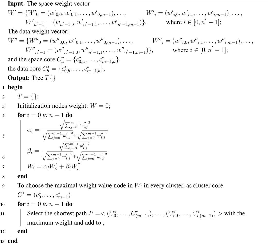
A. To define the weights of the nodes
- Wi,j : The weights of the nodes;
- αi, βi: Linear relation modulus, αi, βi ∈ r; αi, βi ≥ 0, as αi, βi < 0 nonsense;
- W′i : The space weight vector.
- W″i: The data weight vector.
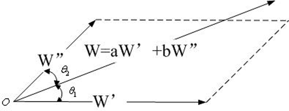
B. The linear relation modulus of the weight of the node satisfied
- Let.
- Take, , .
- Then Wi,j = αiW′i,j + βiW″i,j, and αi + βi = 1, 0 < αi, βi < 1, αi, βi ∈ r
C. The space factor and data factor are game and balance with each other, the game balance point is
D. To get the weight vector and choose the maximum value node as the cluster core
E. Path Weight:
3.4. Multicast Routing Algorithm
| 1 Hence s sends its multicast messages to its cluster core c0. 2 The cluster core c0 sends them to all other cores ci 3 The cluster core c0 routes the multicast packets to its own cluster members along the cluster tree. 4 At the same time, all cluster cores ci, upon receiving the multicast messages, transmit them along the cluster trees to all cluster members mi within the clusters. |
4. Performance Evaluation
4.1. The Model of Simulation
4.2. The Result of Simulation
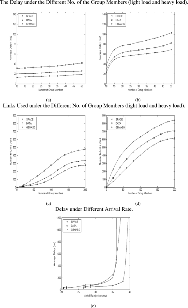
- Under the light load circumstance, the delay is mainly decided by the distance from the source to the group members Figure 7(a). The SPACE approach always transmits multicast packets to group members along the shortest paths from the source to the group members, therefore it achieves the best delay performance among the other systems when the network is lightly loaded. When the traffic is low, GBMASG achieves as good delay performance as SPACE, but with a little bit difference. DATA’s performance is not very good for light load.
- Under a heavy load circumstance, the delay is mainly decided by the source of the data quantity, and certainly relates to the space of the nodes too Figure 7(b). In the sensor grid circumstance, a majority of data quantity will concentrate in minor nodes. Now that SPACE just generate the multicast tree according to space factor, so that the delay increases a little rapidly in the mass data quantity. Our approach GBMASG synthetically considers both data and space factors, so that it gets the best result. DATA achieves the quite well delay performance almost as GBMASG here Figure 7(b).
- Figure 7(c),(d) show the average number of links used by these approaches. In general the number of links will be increased with the number of the group members. At light load, the delay is mainly decided by the distance from the source to the group members Figure 7(c). Therefore SPACE achieves the least the number of links compared with other approach when the network is lightly loaded. GBMASG is in middle and approaching SPACE, but DATA is not very good.
- At heavy load, the number of links is mainly decided by both the source of the data quantity and the space of the node Figure 7(d). So that for SPACE the number of links increases rapidly in the mass data quantity, and the DATA is much better, at last our approach GBMASG get the least the number of links.
- Figure 7(e) shows that the delay increases as the packet arrival-rate increases. The system saturation points for SPACE, DATA and GBMASG are about 35, 36 and 38 packets/ms respectively. Our algorithm GBMASG achieves the maximum throughput.
5. Conclusions and Future Work
5.1. Conclusions
- Cluster formation algorithm. It divides the group members into different clusters in terms of static delay distance;
- Relative weight vectors generation algorithm. It figures out two weight vectors: the space weight vector W′ and the data weight vector W″. In addition, it generates the spatial core Ci,a, which is the node with the maximum space weight node, and the data core Ci,b, which is the node with the maximum space weight node also.
- Least weighted path tree algorithm. After the Relative Weighted Vectors Generation algorithm generates the space weight vector W′ and the data weight vector W″, and the data core Ci,a and the spatial core Ci,b, the sub-algorithm wants to combine the two old weight vectors W′ and W″ to a new weight vector W. But the system just knows W = f(W′, W″), but does not know the expression of the f(). The relationship between the two vectors W′ and W″ can have various forms. We can start the step by discussing the most simple way: the linear relationship, which can represent the typical basic prototype of our real world: W = αW′ + βW″. After that, the sub-algorithm builds binary simple equations, resolves linear parameters α, β, generates new weight vector W. At last generates the least weighted path tree as multicast tree.
- Multicast Routing Algorithm. Firstly, the network is partitioned into clusters in terms of some regular sensor grid area. After group members are initially scattered into different clusters, a tree is built to connect the cluster members within each cluster. At last, the connection among different clusters is done through hooking the tree roots to implement the inter-cluster routing.
5.2. Future Work
1. To extend the multicast algorithm from 2-D to 3-D space
2. To extend the data quantity weight vector W″
3. To discuss the non-linear relationship of two vectors W′ and W″
4. To extend to 3 vectors correlation
5. To extend to N-vectors correlation
Acknowledgments
References
- Duff, R.; Khamra, Y.E. A sensor and computation grid enabled engineering model for drilling vibration research. MG ’08: Proceedings of the 15th ACM Mardi Gras conference, Baton Rouge, Louisiana, USA, January 29–February 03, 2008; p. 153.
- Iqbal, M.; Lim, H.B. A sensor grid infrastructure for large-scale ambient intelligence. PDCAT ’08: Proceedings of the 2008 Ninth International Conference on Parallel and Distributed Computing, Applications and Technologies, Dunedin, New Zealand, December 1–4, 2008; pp. 468–473.
- Bernstein, P.A.; Fekete, A.; Guo, H.; Ramakrishnan, R.; Tamma, P. Relaxed-currency serializability for middle-tier caching and replication. SIGMOD ’06: Proceedings of the 2006 ACM SIGMOD international conference on Management of data, Chicago, IL, USA, June 27–29, 2006; pp. 599–610.
- Pompili, D.; Lopez, L.; Scoglio, C. DIMRO, a DiffServ-integrated multicast algorithm for Internet resource optimization in source specific multicast applications. IEICE Trans. Commun 2004, 2, 1146–1150. [Google Scholar]
- Banerjee, S.; Bhattacharjee, B.; Kommareddy, C. Scalable application layer multicast. Proceedings ACM SIGCOMM, Pittsburgh, Pennsylvania, USA, August 19–23, 2002; pp. 1389–1400.
- Chen, S.; Shi, B. ACOM: Any-source Capacity-constrained Overlay Multicast in Non-DHT P2P Networks. IEEE Trans. Paral. Dis. Sys 2007, 18, 205–217. [Google Scholar]
- Zhuge, H. A Scalable P2P Platform for the Knowledge Grid. IEEE Trans. Know. Da. Eng 2005, 17, 1721–1736. [Google Scholar]
- Nakao, A.; Peterson, L.; Bavier, A. A routing underlay for overlay networks. Proceedings of ACM SIGCOMM, Karlsruhe, Germany, August 25–29, 2003; pp. 1175–1209.
- Shavitt, Y.; Tankel, T. Big-bang simulation for embedding network distances in Euclidean space. IEEE ACM Trans. Networking 2004, 12, 993–1006. [Google Scholar]
- Zhang, H.; Kurose, J.; Towsley, D. Can an overlay compensate for a careless underlay? Proceedings of IEEE INFOCOM, Barcelona, Spain, April 23–29, 2006; pp. 1–12.
- Zissimos, A.; Doka, K.; Chazapis, A.; Koziris, N. GridTorrent: Optimizing data transfers in the Grid with collaborative sharing. Proceedings of 11th Panhellenic Conference on Informatics (PCI2007), Nuremberg, Germany, May 18–20, 2007; pp. 2–5.
- Chu, Y.; Rao, S.G.; Seshan, S.; Zhang, H. Enabling conferencing applications on the Internet using an overlay multicast architecture. ACM SIGCOMM 2001, 153, 55–67. [Google Scholar]
- Birman, K.P. Scalable trust: engineering challenge or complexity barrier? Proceedings of the first ACM workshop on Scalable trusted computing, Alexandria, VA, USA, November 3, 2006; pp. 1–2.
- Waters, G.; Crawford, J.; Lim, S.G. Optimising multicast structures for grid computing. Compt. Commun 2004, 27, 1389–1400. [Google Scholar]
- Bell, G.; Gray, J.; Szalay, A. Petascale computational systems. Proceedings of IEEE INFOCOM, Barcelona, Catalunya, Spain, April 23–29, 2006; pp. 110–112.
- Akbarinia, R.; Esther, P.; Patrick, V. Data currency in replicated DHTs. SIGMOD ’07: Proceedings of the 2007 ACM SIGMOD international conference on Management of data, Beijing, China, June 11–14, 2007; pp. 1389–1400.
- Mouratidis, K.; Bakiras, S.; Papadias, D. Continuous monitoring of top-k queries over sliding windows. ACM Trans. Data Sys 2006, 31, 1095–1133. [Google Scholar]
- Akbarinia, R.; Esther, P.; Patrick, V. Best position algorithms for top-k queries. VLDB ’07:Proceedings of the 33rd international conference on Very large data bases, Vienna, Austria, September 23–28, 2007; pp. 1389–1400.
- Ye, B.; Guo, M.; Zhou, J.; Chen, D. A multicast based anonymous information sharing protocol for peer-to-peer systems. IEICE Trans. Inform. Sys 2006, E89-D, 581–588. [Google Scholar]
- Jia, W.; Tu, W.; Wu, J. Hierarchical Multicast Tree Algorithms for Application Layer Mesh Networks. Proceedings of 2006 International Conference on Computer Networks and Mobile Computing, Los Angeles, CA, USA, September 23–29, 2006; pp. 967–971.
- Setton, E.; Noh, J.; Girod, B. Rate-distortion optimized video peer-to-peer multicast streaming. Proceedings of the ACM workshop on Advances in peer-to-peer multimedia streaming multimedia streaming, Hilton, Singapore, November 11, 2005; pp. 160–172.
- Stocia, I.; Morris, R.; Karger, D.; Kaashoek, M.F.; Balakrishnan, H. Chord: A scalable peer-to-peer lookup service for internet applications. Proceedings of ACM SIGCOMM, San Diego, CA, USA, August 27–31, 2001; pp. 160–172.
- Tu, W.; Jia, W. A scalable and efficient end host multicast for Peer-to-Peer Systems. Proceedings of IEEE Globecom, Dallas, Texas, USA, November 29–December 3, 2004; pp. 967–971.
- Zhang, Y.; Roughan, M.; Duffield, N.; Greenberg, A. Fast accurate computation of large-scale IP traffic matrices from link loads. ACM SIGMETRICS 2003, 31, 206–217. [Google Scholar]
- Jia, W. Implementation of a Reliable Multicast Protocol. Software-Pract. Exper 1997, 27, 813–850. [Google Scholar]
- Lazarevic, A.; Pokrajac, D.; Obradovic, Z. Distributed clustering and local regression for knowledge discovery in multiple spatial databases. Proceedings of Eighth European Symposium on Artificial Neural Networks, Bruges, Belgium, April 26–28, 2000; pp. 129–134.
- Wei, B.; Fedak, G.; Cappello, F. Scheduling Independent Tasks Sharing Large Data Distributed with BitTorrent. Proceedings of the 6th IEEE/ACM International Workshop on Grid Computing, Seattle, WA, USA, November 13–14, 2005; pp. 219–226.


| Y=6 | 0 | 1* | 0 | 0 | 0 |
| Y=5 | 0 | 3 | 2* | 1 | 1* |
| Y=4 | 0 | 4* | 2 | 1 | 1 |
| Y=3 | 1* | 5 | 2 | 1 | 1 |
| Y=2 | 2 | 10* | 4 | 2 | 2* |
| Y=1 | 1* | 3* | 1* | 0 | 0 |
| X=1 | X=2 | X=3 | X=4 | X=5 |
| Y=6 | 0 | 1* | 0 | 0 | 0 |
| Y=5 | 0 | 3 | 2* | 1 | 0* |
| Y=4 | 0 | 5* | 2 | 2 | 1 |
| Y=3 | 2* | 4 | 3 | 2 | 1 |
| Y=2 | 2 | 1* | 4 | 3 | 2* |
| Y=1 | 3* | 10* | 3* | 0 | 0 |
| X=1 | X=2 | X=3 | X=4 | X=5 |
| Y=6 | 0 | 1.00* | 0 | 0 | 0 |
| Y=5 | 0 | 3 | 2.00* | 1 | 0.53* |
| Y=4 | 0 | 4.47* | 2 | 2 | 1 |
| Y=3 | 1.47* | 4 | 3 | 2 | 1 |
| Y=2 | 2 | 5.79* | 4 | 3 | 2.00* |
| Y=1 hline | 1.94* X=1 | 6.27* X=2 | 1.94* X=3 | 0 X=4 | 0 X=5 |
© 2009 by the authors; licensee MDPI, Basel, Switzerland This article is an open access article distributed under the terms and conditions of the Creative Commons Attribution license (http://creativecommons.org/licenses/by/3.0/).
Share and Cite
Fan, Q.; Wu, Q.; Magoulés, F.; Xiong, N.; Vasilakos, A.V.; He, Y. Game and Balance Multicast Architecture Algorithms for Sensor Grid. Sensors 2009, 9, 7177-7202. https://doi.org/10.3390/s90907177
Fan Q, Wu Q, Magoulés F, Xiong N, Vasilakos AV, He Y. Game and Balance Multicast Architecture Algorithms for Sensor Grid. Sensors. 2009; 9(9):7177-7202. https://doi.org/10.3390/s90907177
Chicago/Turabian StyleFan, Qingfeng, Qiongli Wu, Frèdèric Magoulés, Naixue Xiong, Athanasios V. Vasilakos, and Yanxiang He. 2009. "Game and Balance Multicast Architecture Algorithms for Sensor Grid" Sensors 9, no. 9: 7177-7202. https://doi.org/10.3390/s90907177