3.1. Assumption
Similar to the assumption in [
3], let us consider a sensor network with
M static sensor nodes in a 2D plane which do not have
a priori known locations (called
unknown nodes) and a single mobile node (called
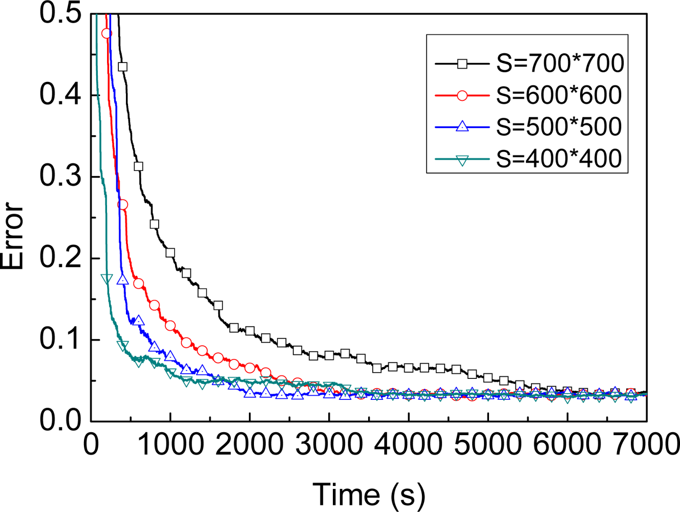
beacon), equipped with localization hardware, e.g., a GPS, which allows it to know its location at all times. We assume that all unknown nodes are randomly deployed in an area of size
S and each sensor (unknown node or beacon) has the same ideal radio range
r. The beacon is capable of moving a distance in a time step (
vb) in any direction where 0 ≤
vb ≤
vmax. The beacon knows
vmax, but it does not know the value of
vb or the direction of movement in any time step. At time
t, every unknown node within the radio range of the beacon will hear a location announcement from that beacon. We do not assume very tightly synchronized clocks. In a realistic deployment, it would be necessary to deal with network collisions and account for missed messages [
18].
3.2. A-MBL
A-MBL uses the
particle filter approach (also called
sequential Monte Carlo method) to perform Bayesian filter based localization on a sample representation. The key idea is to represent the required posterior density by a set of random samples with associated weights and to compute estimates based on these samples and weights [
19].
Let
denotes a random measure that characterizes the posterior density p(lt | ot) which denotes the current location estimate lt conditioned on the observation ot from the beacon at time t, where
denotes a set of support samples (or called particles) with associated weights at time t and N denotes the number of samples of an unknown node.
The details of the A-MBL are as follows:
Initialization: In this stage, all unknown nodes have no information about their locations. The initial set of samples
Equation 1 for each unknown node is chosen randomly from the whole deployed area and represented by a set of uniformly distributed samples with equal weights
Equation 2. The weight equal to one represents the importance of corresponding sample, which infers one of the location estimates of the unknown node:
where
L0 denotes the initial set of each sample,
p(
l0) denotes initial location probability density, the symbol ∼ denotes sample generated sign, i.e., the samples on the left side are generated from the probability density on the right side, and
denotes the initial weight of each sample.
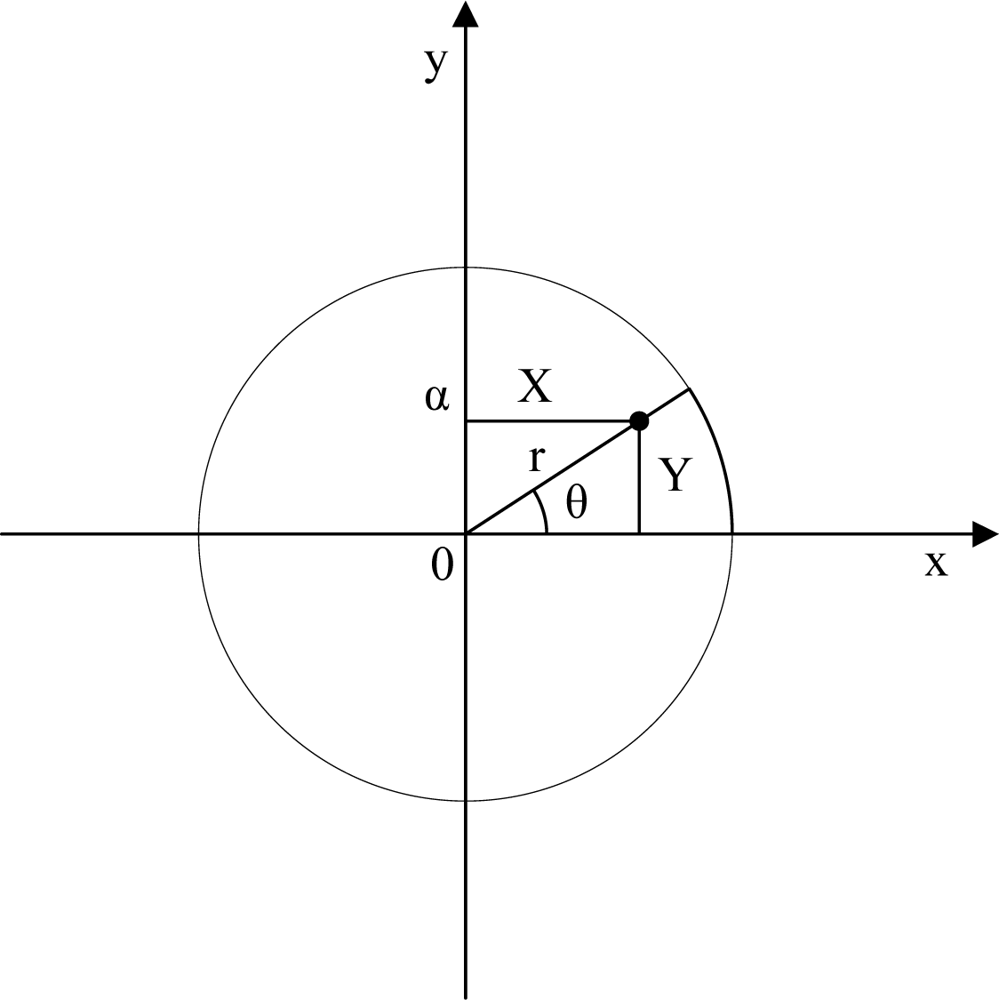
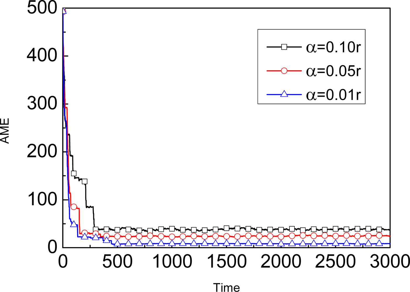
Prediction: In this stage, we adopt a
dynamic model in which the unknown node is capable of moving a distance in a time step (
vnode) in any direction where 0 ≤
vnode ≤ α. The unknown node knows α, but it does not know the value of
vnode or the direction of movement in any time step. Then, the unknown node generates new samples as follows:
where
Pt represents the approximation of prior density at time
t after the prediction stage,
Lt−1 represents the approximation of posterior density at time
t−1, and the
transition equation for each sample described as follows:
where
filter(R) denotes the unknown node receives the current location announcement of the beacon, but did not receive the location announcement from the beacon’s previous location, or the unknown node received the preceding location announcement from the beacon, but does not receive the location announcement from the beacon’s current location. For more details about
filter(R) see [
3].
Update: In this stage, the unknown node filters the impossible samples based on new observations. The unknown node updates samples as follows:
where
Ut represents the approximation of posterior density at time
t after the update stage, and the weight
will be obtained by
. The weight of sample is determined by the filter condition:
Resampling: A-MBL adopts a Systematic resampling algorithm [
20] in this paper since it is simple to implement, takes
O(Ns) time, and minimizes the Monte Carlo variation.
Adapting: A-MBL adopts two predefined adjustment tables, one for the number of samples N, and the other for the parameter α. Once some record in the table is matched, the number of samples and the value of α in the unknown node will be adjusted according to the corresponding time.
The complete A-MBL for every unknown node is shown in [
3].


