An Efficient and Self-Adapting Localization in Static Wireless Sensor Networks


Abstract
:1. Introduction
Dynamic model
Neighbors’ observation
Adapting mechanism
- In order to improve the time efficiency in the prediction stage of particle filter-based mobile beacon-assisted localization, we give the theoretical analysis and experimental evaluations to suggest which probability distribution should be adopted in the dynamic model.
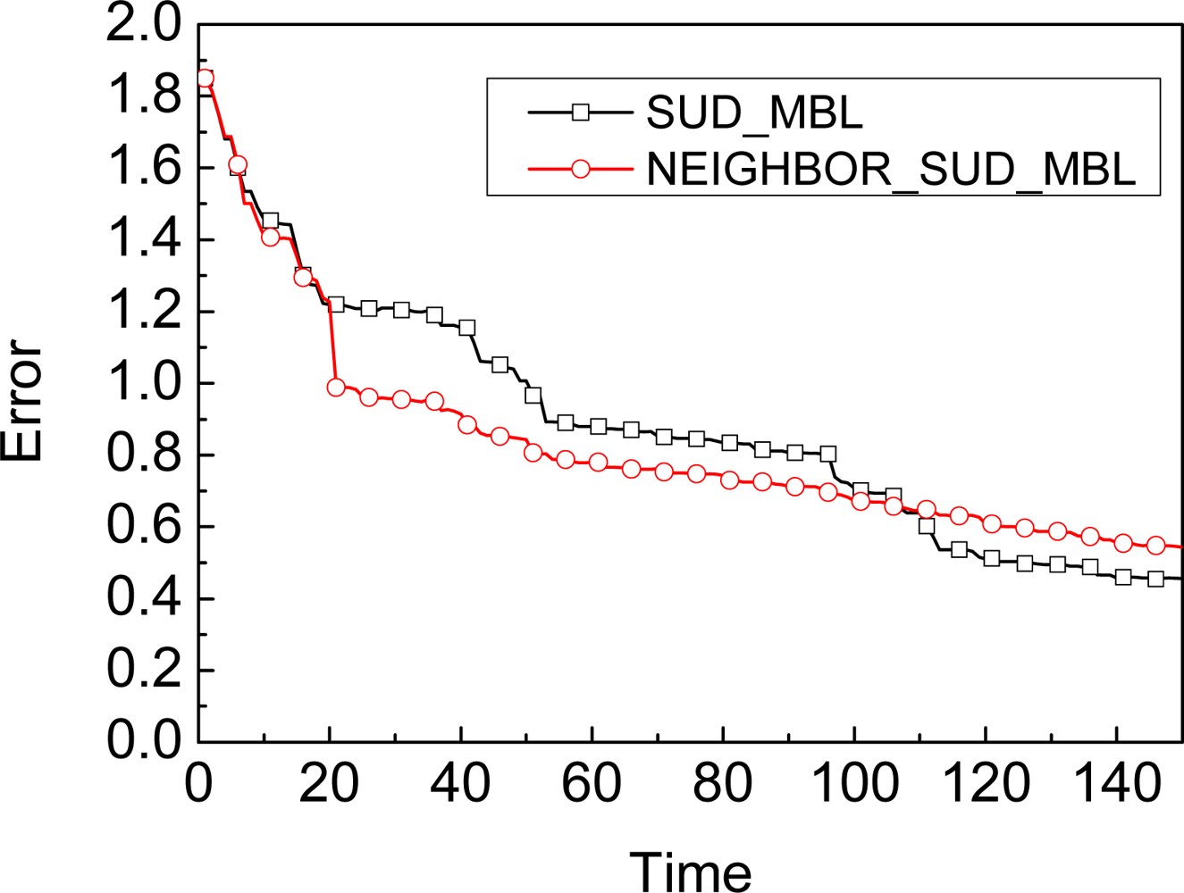
- We give the condition for whether the unknown node should use the observation from its neighbors to improve the accuracy.
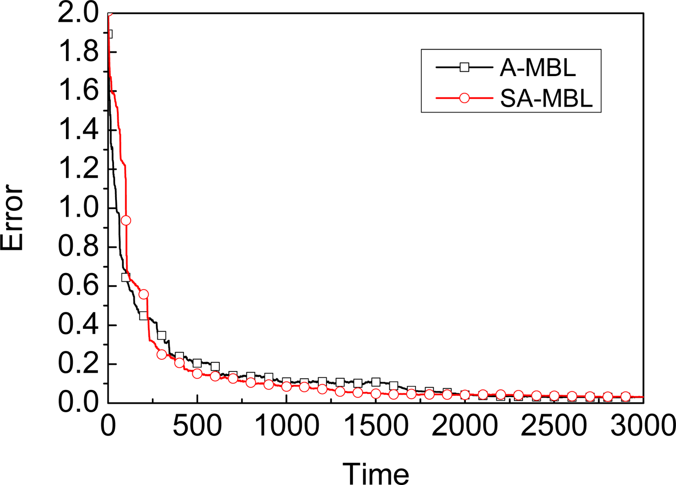
- We propose a Self-Adapting Mobile Beacon-assisted Localization (SA-MBL) approach to achieve more flexibility and obtain almost the same performance as with A-MBL.
2. Related Work
3. Description of A-MBL
3.1. Assumption
3.2. A-MBL
4. Key Issues
4.1. Dynamic Model
4.1.1. Square uniform distribution
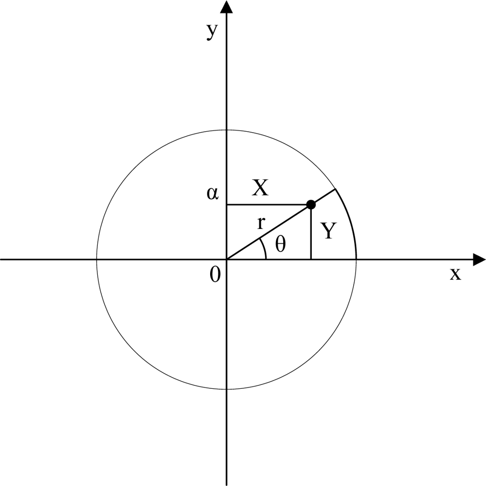
4.1.2. Circle uniform distribution

| 1: do |
| 2: Generate random numbers U1 and U2; |
| 3: X = −α + 2α*U1, Y = −α + 2α*U2; |
| 4: While X2 + Y2 ≥ r2 |
| 5: Accept X, Y; |
4.1.3. Normal distribution
| 1: do |
| 2: Generate random numbers U1 and U2; |
| 3: Set V1 = 2U1 −1, V2 = 2U2 −1, ; |
| 4: While S > 1 |
| 5: |
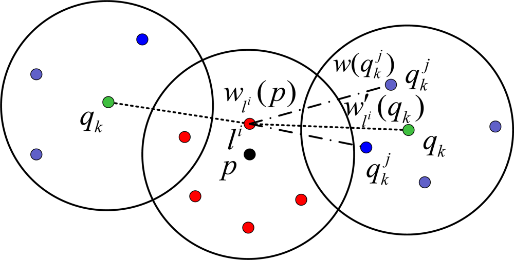
4.2. Neighbors’ Observation
- If the unknown node receives the observation from the beacon, then the partial weight w′li (qk) of sample li will be computed by the Equation 6 as MBL (or A-MBL).
- If the unknown node receives the observations from its neighbors, then the partial weight w′li (qk) of the sample li corresponding to the neighbor qk is computed using the weights of the sample of the neighbor qk as follows:
4.3. Self-Adapting Mechanism
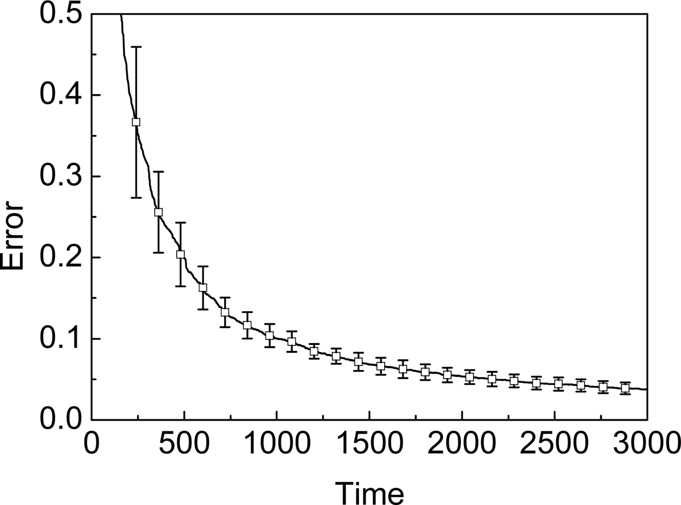
- The approach should judge the localization to reach the stable phase as the effect of pre-defined table in A-MBL.
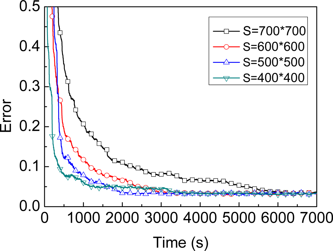
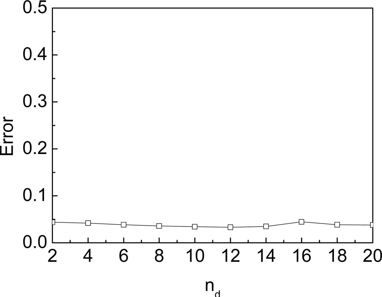
- The approach should be unrelated to the scale deployment of sensor nodes, the localization time, and the speed of the beacon, etc., but just related to the unknown nodes themselves.
5. Evaluation
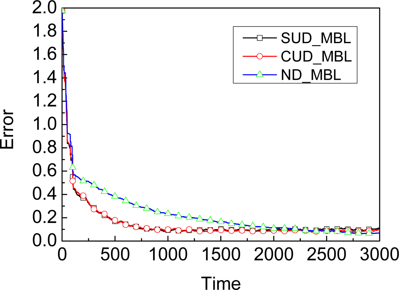
5.1. Dynamic Model
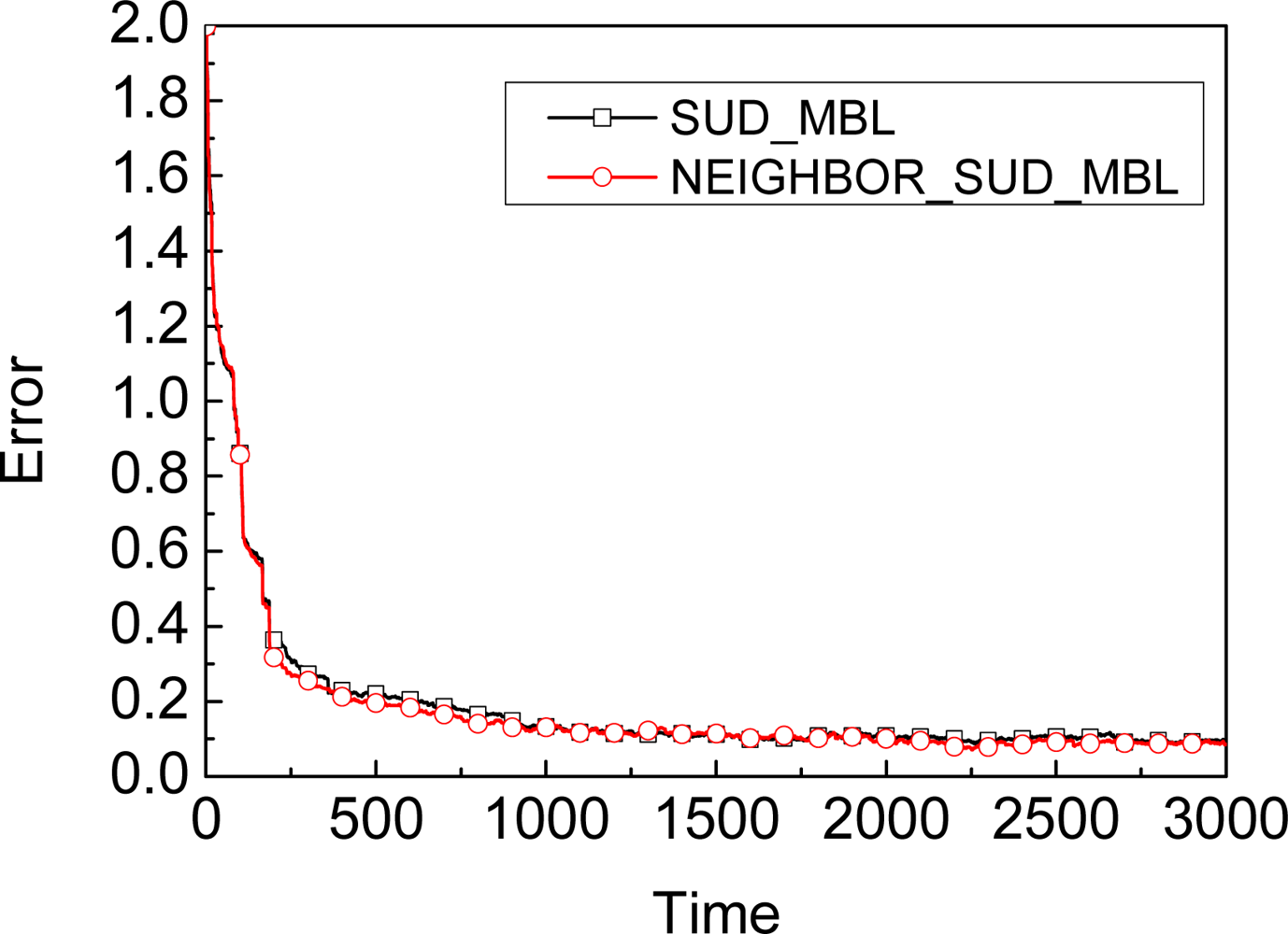
5.2. Neighbors’ Observation
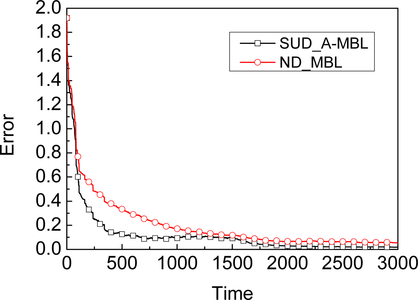
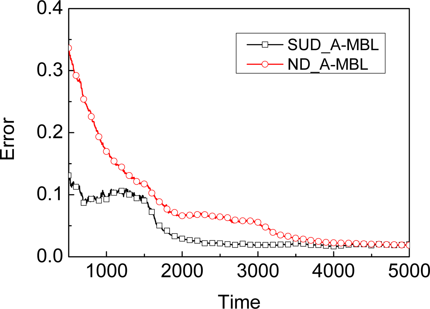
5.3. SA-MBL
6. Conclusions
Acknowledgments
References
- Akyildiz, I.F.; Su, W.; Sankarasubramaniam, Y.; Cayirci, E. A survey on sensor networks. IEEE Commun. Mag 2002, 40, 102–114. [Google Scholar]
- Hightower, J.; Borriello, G. Location systems for ubiquitous computing. IEEE Comput 2001, 34, 57–66. [Google Scholar]
- Teng, G.; Zheng, K.; Dong, W. Adapting mobile beacon-assisted localization in wireless sensor networks. Sensors 2009, 9, 2760–2779. [Google Scholar]
- Priyantha, N.B.; Balakrishnan, H.; Demaine, E.D.; Teller, S. Mobile-assisted Localization in Wireless Sensor Networks. Proceedings of The 24th Annual Joint Conference of the IEEE Computer and Communications Societies, Miami, FL, USA, 2005; pp. 172–183.
- Kim, K.; Lee, W. MBAL: A Mobile Beacon-assisted Localization Scheme for Wireless Sensor Networks. Proceedings of The 16th International Conference on Computer Communications and Networks, Honolulu, HI, USA, 2007; pp. 57–62.
- Sichitiu, M.L.; Ramadurai, V. Localization of Wireless Sensor Networks with a Mobile Beacon. Proceedings of The First IEEE Conference on Mobile Ad-hoc and Sensor Systems, Philadelphia, PA, USA, 2004; pp. 174–183.
- Caballero, F.; Merino, L.; Maza, I.; Ollero, A. A Particle Filtering Method for Wireless Sensor Network Localization with an Aerial Robot Beacon. Proceedings of IEEE International Conference on Robotics and Automation, Pasadena, CA, USA, 2008; pp. 596–601.
- Marinakis, D.; Meger, D.; Rekleitis, I.; Dudek, G. Hybrid Inference for Sensor Network Localization Using a Mobile Robot. Proceedings of the Twenty-Second AAAI Conference on Artificial Intelligence, Vancouver, BC, Canada, 2007; pp. 1089–1094.
- Ihler, A.T.; Fisher, J.W.; Moses, R.L.; Willsky, A.S. Nonparametric belief propagation for self-localization of sensor networks. IEEE J. Sel. Area Comm 2005, 23, 809–819. [Google Scholar]
- Peng, R.; Sichitiu, M.L. Robust, Probabilistic, Constraint-Based Localization for Wireless Sensor Networks. Proceedings of The Second Annual IEEE Sensor and Ad Hoc Communications and Networks, Santa Clara, CA, USA, 2005; pp. 541–550.
- Li, M.; Liu, Y. Rendered Path: Range-Free Localization in Anisotropic Sensor Networks with Holes. Proceedings of The 13th Annual ACM International Conference on Mobile Computing and Networking, Montreal, QU, Canada, 2007; pp. 51–62.
- Stoleru, R.; He, T.; Stankovic, J.A. Walking gps: A Practical Solution for Localization in Manually Deployed Wireless Sensor Networks. Proceedings of The 29th Annual IEEE International Conference on Local Computer Networks, Tampa, FL, USA, 2004; pp. 480–489.
- Xiao, B.; Chen, H.K.; Zhou, S.G. A Walking Beacon-assisted Localization in Wireless Sensor Networks. Proceedings of International Conference on Communications, Glasgow, Scotland, 2007; pp. 3070–3075.
- Huang, R.; Zruba, G.V. Monte carlo localization of wireless sensor networks with a single mobile beacon. Wirel. Netw 2008. [Google Scholar] [CrossRef]
- Teng, G.; Zheng, K.; Dong, W. MA-MCL: Mobile-Assisted Monte Carlo Localization for Wireless Sensor Networks. Proceedings of The 4th Int'l Symp. on Innovations and Real-time Applications of Distributed Sensor Networks, Hangzhou, China, 2009; pp. 148–155.
- Rudafshani, M.; Datta, S. Localization in Wireless Sensor Networks. Proceedings of the 6th International Conference on Information Processing in Sensor Networks, Cambridge, MA, USA, 2007; pp. 51–60.
- Woo, A.; Tong, T.; Culler, D. Taming the Underlying Challenges of Reliable Multihop Routing in Sensor Networks. Proceedings of the First International Conference on Embedded Networked Sensor Systems, Los Angeles, CA, USA, 2003; pp. 14–27.
- Hu, L.; Evans, D. Localization for Mobile Sensor Networks. Proceedings of the 10th Annual International Conference on Mobile Computing and Networking, New York, NY, USA, 2004; pp. 45–57.
- Arulampalam, S.; Maskell, S.; Gordon, N. A tutorial on particle filters for online nonlinear/non-gaussian bayesian tracking. IEEE Trans. Signal Process 2002, 50, 174–188. [Google Scholar]
- Kitagawa, G. Monte carlo filter and smoother for non-gaussian nonlinear state space models. J. Comput. Graph. Stat 1996, 5, 1–25. [Google Scholar]
- Ross, S.M. Introduction to Probability Models, Ninth Edition ed; Academic Press: Burlington, MA, USA, 2006; pp. 663–680. [Google Scholar]
- Nagpal, R.; Shrobe, H.; Bachrach, J. Organizing a Global Coordinate System from Local Information on an Ad Hoc Sensor Network. Proceedings of Second International Workshop on Information Processing in Sensor Networks, Palo Alto, CA, USA, 2003; pp. 333–348.
- Fox, D.; Burgard, W.; Dellaert, F. Monte Carlo Localization: Efficient Position Estimation for Mobile Robots. Proceedings of The Sixteenth National Conference on Artificial Intelligence, Orlando, FL, USA, 1999; pp. 343–349.
- Fox, D. Adapting the sample size in particle filters through KLD-sampling. Int. J. Rob. Res 2003, 22, 985–1003. [Google Scholar]


| Probability Distribution | UD (Uniform Distribution) | ND (Normal Distribution) | |||
|---|---|---|---|---|---|
| SUD | CUD | ||||
| Simulation Method | Accept-Reject | Polar | Box-Muller | Polar | |
| Random Numbers | 2 | 2.546 | 2 | 2 | 2.546 |
| Trigonometric Function | 0 | 0 | 2 | 2 | 0 |
| Logarithm | 0 | 0 | 0 | 1 | 1 |
| Square Root | 0 | 0 | 1 | 1 | 1 |
| Multiplication | 4 | 7.638 | 5 | 6 | 10.638 |
| Division | 0 | 0 | 0 | 0 | 1 |
| Name | SUN_MBL | CUD_MBL | ND_MBL |
|---|---|---|---|
| Error | 0.097430 | 0.090572 | 0.073601 |
| Time | 106 | 208 | 500 | 1000 | 2000 | 3000 |
|---|---|---|---|---|---|---|
| Number | 10 | 20 | 45 | 91 | 176 | 260 |
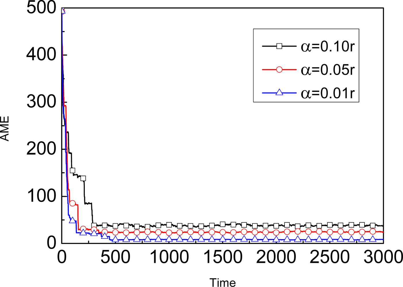
| No. | α | N | AME |
|---|---|---|---|
| 1 | 0.10r | 50 | 38.749791 |
| 2 | 0.09r | 50 | 36.766873 |
| 3 | 0.08r | 40 | 34.275935 |
| 4 | 0.07r | 40 | 30.948355 |
| 5 | 0.06r | 30 | 28.403102 |
| 6 | 0.05r | 30 | 24.881642 |
| 7 | 0.04r | 20 | 21.765849 |
| 8 | 0.03r | 20 | 18.161460 |
| 9 | 0.02r | 10 | 13.720697 |
| 10 | 0.01r | 10 | 08.323300 |
© 2009 by the authors; licensee MDPI, Basel, Switzerland This article is an open access article distributed under the terms and conditions of the Creative Commons Attribution license (http://creativecommons.org/licenses/by/3.0/).
Share and Cite
Teng, G.; Zheng, K.; Dong, W. An Efficient and Self-Adapting Localization in Static Wireless Sensor Networks. Sensors 2009, 9, 6150-6170. https://doi.org/10.3390/s90806150
Teng G, Zheng K, Dong W. An Efficient and Self-Adapting Localization in Static Wireless Sensor Networks. Sensors. 2009; 9(8):6150-6170. https://doi.org/10.3390/s90806150
Chicago/Turabian StyleTeng, Guodong, Kougen Zheng, and Wei Dong. 2009. "An Efficient and Self-Adapting Localization in Static Wireless Sensor Networks" Sensors 9, no. 8: 6150-6170. https://doi.org/10.3390/s90806150
APA StyleTeng, G., Zheng, K., & Dong, W. (2009). An Efficient and Self-Adapting Localization in Static Wireless Sensor Networks. Sensors, 9(8), 6150-6170. https://doi.org/10.3390/s90806150