Orientation of Airborne Laser Scanning Point Clouds with Multi-View, Multi-Scale Image Blocks

Abstract
:
1. Introduction
2. Materials
3. Methods
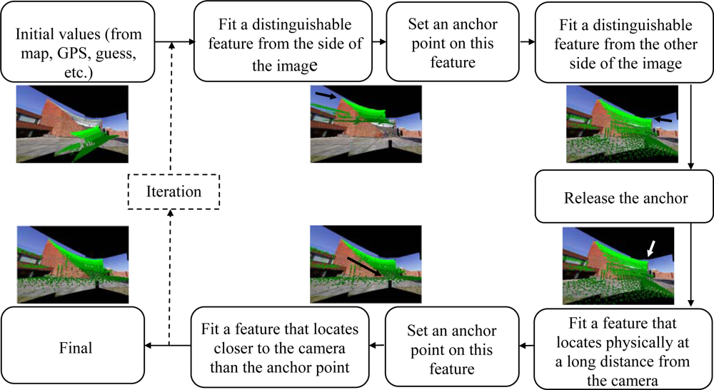
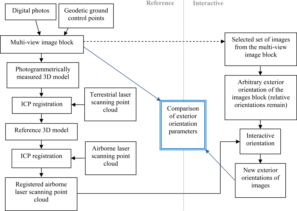
3.1. Workflow
3.2. Reference Orientation for Laser Scanning Data
3.3. The Interactive Orientation of a Laser Point Cloud and a Multi-view Image Block
3.4. Applying Transformations to Laser Point Clouds
4. Results and Discussion
4.1. The Accuracy of an Interactive Orientation of Multi-view Image Blocks and Laser Scanning Data
4.2. Integrated Multi-source Data
4.3. Confirmation of the Inverse Transformation from Image Orientations to Laser Scanning Point Cloud Transformations
5. Conclusions
Acknowledgments
References and Notes
- Böhm, J.; Haala, N. Efficient Integration of Aerial and Terrestrial Laser Data for Virtual City Modeling Using Lasermaps. Int. Arch. Photogramm. Remote Sens 2005, 36, 192–197. [Google Scholar]
- Rönnholm, P.; Hyyppä, H.; Pöntinen, P.; Haggrén, H.; Hyyppä, J. A Method for Interactive Orientation of Digital Images Using Backprojection of 3D Data. Photogramm. J. Finland 2003, 18, 58–69. [Google Scholar]
- Rönnholm, P.; Hyyppä, J.; Hyyppä, H.; Haggrén, H.; Yu, X.; Kaartinen, H. Calibration of Laser-Derived Tree Height Estimates by Means of Photogrammetric Techniques. Scand. J. Forest Res 2004, 19, 524–528. [Google Scholar]
- Rönnholm, P.; Honkavaara, E.; Litkey, P.; Hyyppä, H.; Hyyppä, J. Integration of Laser Scanning and Photogrammetry. Int. Arch. Photogramm. Remote Sens. Spat. Inf. Sci 2007, 36, 355–362. [Google Scholar]
- Kajuutti, K.; Jokinen, O.; Geist, T.; Pitkänen, T. Terrestrial Photography for Verification of Airborne Laser Scanner Data on Hintereisferner in Austria. Nordic J. Surv. Real Estate Res 2007, 4, 24–39. [Google Scholar]
- Kraus, K.; Pfeifer, N. Determination of Terrain Models in Wooded Areas with Airborne Laser Scanner Data. ISPRS J. Photogramm. Remote Sens 1998, 53, 193–203. [Google Scholar]
- Hyyppä, J.; Pyysalo, U.; Hyyppä, H.; Haggren, H.; Ruppert, G. Accuracy of Laser Scanning for DTM Generation in Forested Areas. Proceedings of SPIE Laser Radar Technology and Applications V, Orlando, FL, USA, 2000; 4035, pp. 119–130.
- Reutebuch, S.; McGaughey, R.; Andersen, H.; Carson, W. Accuracy of a High-resolution Lidar Terrain Model under a Conifer Forest Canopy. Can. J. Remot. Sens 2003, 29, 527–535. [Google Scholar]
- Hyyppä, H.; Yu, X.; Hyyppä, J.; Kaartinen, H.; Kaasalainen, S.; Honkavaara, E.; Rönnholm, P. Factors Affecting the Quality of DTM Generation in Forested Areas. Int. Arch. Photogramm. Remote Sens. Spat. Inf. Sci 2005, 36, 97–102. [Google Scholar]
- Ahokas, E.; Kaartinen, H.; Hyyppä, J. On the Quality Checking of the Airborne Laser Scanning-based Nationwide Elevation Model in Finland. Int. Arch. Photogramm. Remote Sens. Spat. Inf. Sci 2008, 37, 267–270. [Google Scholar]
- Sithole, G.; Vosselman, G. Experimental Comparison of Filter Algorithms for Bare-Earth Extraction from Airborne Laser Scanning Point Clouds. ISPRS J. Photogramm. Remote Sens 2004, 59, 85–101. [Google Scholar]
- Brenner, C.; Haala, N. Rapid Acquisition of Virtual Reality City Models from Multiple Data Sources. Int. Arch. Photogramm. Remot. Sens 1998, 32, 323–330. [Google Scholar]
- Vosselman, G. Building Reconstruction Using Planar Faces in Very High Density Data. Int. Arch. Photogramm. Remot. Sens 1999, 32, 87–92. [Google Scholar]
- Brenner, C. Towards Fully Automatic Generation of City Models. Int. Arch. Photogramm. Remot. Sens 2000, 33, 85–92. [Google Scholar]
- Rottensteiner, F.; Briese, C. A New Method for Building Extraction in Urban Areas from High-resolution LIDAR Data. Int. Arch. Photogramm. Remote Sens. Spat. Inf. Sci 2002, 34, 295–301. [Google Scholar]
- Sithole, G.; Vosselman, G. Bridge Detection in Airborne Laser Scanner Data. ISPRS J. Photogramm. Remote Sens 2006, 61, 33–46. [Google Scholar]
- Rutzinger, M.; Höfle, B.; Pfeifer, N. Detection of High Urban Vegetation with Airborne Laser Scanning Data. Proceedings of ForestSat’07, Montpellier, France, 2007; Available online: http://www.ipf.tuwien.ac.at/np/Publications/rutzinger_forestsat.pdf/ (accessed on April 16, 2009).
- Dorninger, P.; Pfeifer, N. A Comprehensive Automated 3D Approach for Building Extraction, Reconstruction, and Regularization from Airborne Laser Scanning Point Clouds. Sensors 2009, 8, 7323–7343. [Google Scholar]
- Boehler, W.; Bordas Vicent, M.; Marbs, A. Investigating Laser Scanner Accuracy. Proceedings of XIXth CIPA Symposium, Antalya, Turkey, 2003; pp. 696–702.
- Hunter, G.; Cox, C.; Kremer, J. Development of a Commercial Laser Scanning Mobile Mapping System – StreetMapper. Int. Arch. Photogramm. Remote Sens. Spat. Inf. Sci. 2006, 36. Available online at: http://www.streetmapper.net/articles/Paper%20-%20Development%20of%20a%20Commercial%20Laser%20Scanning%20Mobile%20Mapping%20System%20-%20Pegasus.pdf/ (accessed on April 16, 2009).
- Kukko, A. Road Environment Mapper - 3D Data Capturing with Mobile Mapping, Licentiate Thesis.. Department of Surveying, Helsinki University of Technology, Espoo, Finland, 2009.
- Kremer, J. CCNS and AEROcontrol: Products for Efficient Photogrammetric Data Collection. In Photogrammetric Week 2001; Fritsch, D, Spiller, R., Eds.; Wichmann Verlag: Heidelberg, Germany, 2001; pp. 85–92. [Google Scholar]
- Heipke, C.; Jacobsen, K.; Wegmann, H. Analysis of the Results of the OEEPE Test Integrated Sensor Orientation. OEEPE Official Publication.. 2002, 43, pp. 31–45. Avalable online: http://www.gtbi.net/export/sites/default/GTBiWeb/soporte/descargas/AnalisisOeepeOrientacionIntegrada-en.pdf/ (accessed on April 16, 2009).
- Honkavaara, E.; Ilves, R.; Jaakkola, J. Practical Results of GPS/IMU/Camera-system Calibration. Proceedings of International Workshop: Theory, Technology and Realities of Inertial/GPS Sensor Orientation, Castelldefels, Spain, 2003; Avalable online: http://www.isprs.org/commission1/theory_tech_realities/pdf/p06_s3.pdf/ (accessed on 16 April 2009).
- Hutton, J.; Bourke, T.; Scherzinger, B.; Hill, R. New developments of inertial navigation system at applanix. In Photogrammetric Week ’07; Fritsch, D., Ed.; Wichmann Verlag: Heidelberg, Germany, 2007; pp. 201–213. [Google Scholar]
- Jacobsen, K. Direct Integrated Sensor Orientation – Pros and Cons. Int. Arch. Photogramm. Remote Sens. Spat. Inf. Sci 2004, 35, 829–835. [Google Scholar]
- Merchant, D.; Schenk, A.; Habib, A.; Yoon, T. 2004. USGS/OSU Progress with Digital Camera in situ Calibration Methods. Int. Arch. Photogramm. Remote Sens 2004, 35, 19–24. [Google Scholar]
- Schenk, T. Towards Automatic Aerial Triangulation. ISPRS J. Photogramm. Remote Sens 1997, 52, 110–121. [Google Scholar]
- Alamús, R.; Kornus, W. DMC Geometry Analysis and Virtual Image Characterization. Photogramm. Rec 2008, 23, 353–371. [Google Scholar]
- Püschel, H.; Sauerbier, M.; Eisenbeiss, H. A 3D Model of Castle Landenberg (CH) from Combined Photogrammetric Processing of Terrestrial and UAV-based Images. Int. Arch. Photogramm. Remote Sens. Spat. Inf. Sci 2008, 37, 93–98. [Google Scholar]
- Zhu, L.; Erving, A.; Koistinen, K.; Nuikka, M.; Junnilainen, H.; Heiska, N.; Haggrén, H. Georeferencing Multi-temporal and Multi-scale Imagery in Photogrammetry. Int. Arch. Photogramm. Remote Sens. Spat. Inf. Sci 2008, 37, 225–230. [Google Scholar]
- Lichti, D.; Licht, G. Experiences with Terrestrial Laser Scanner Modelling and Accuracy Assessment. Int. Arch. Photogramm. Remote Sens. Spat. Inf. Sci 2006, 36, 155–160. [Google Scholar]
- Brenner, C.; Dold, C.; Ripperda, N. Coarse Orientation of Terrestrial Laser Scans in Urban Environments. ISPRS J. Photogramm. Remote Sens 2008, 63, 4–18. [Google Scholar]
- Besl, P.; McKay, N. A Method for Registration of 3D Shapes. IEEE Trans. Patt. Anal. Machine Intell 1992, 14, 239–256. [Google Scholar]
- Chen, Y.; Medioni, G. Object Modeling by Registration of Multiple Range Images. Image Vis. Comp 1992, 10, 145–155. [Google Scholar]
- Eggert, D.; Fitzgibbon, A.; Fisher, R. Simultaneous Registration of Multiple Range Views for Use in Reverse Engineering of CAD Models. Comp. Vis. Image Underst 1998, 69, 253–272. [Google Scholar]
- Akca, D. Registration of Point Clouds Using Range and Intensity Information. The International Workshop on Recording, Modeling and Visualization of Cultural Heritage, Ascona, Switzerland, 2005; pp. 115–126.
- Pfeifer, N. Airborne Laser Scanning Strip Adjustment and Automation of Tie Surface Measurement. Bol. Ciênc. Geod 2005, 11, 3–22. [Google Scholar]
- Csanyi, N.; Toth, C. Improvement of Lidar Data Accuracy Using Lidar-specific Ground Targets. Photogramm. Eng. Remote Sens 2007, 73, 385–396. [Google Scholar]
- Yastikli, N.; Toth, C.; Brzezinska, D. Multi Sensor Airborne Systems: the Potential for in situ Sensor Calibration. Int. Arch. Photogramm. Remote Sens. Spat. Inf. Sci 2008, 37, 89–94. [Google Scholar]
- Hyyppä, H.; Rönnholm, P.; Soininen, A.; Hyyppä, J. Scope for Laser Scanning to Provide Road Environment Information. Photogramm. J. Finland 2005, 19, 19–33. [Google Scholar]
- Toth, C.; Paska, E.; Brzezinska, D. Using Pavement Markings to Support the QA/QC of Lidar Data. Int. Arch. Photogramm. Remote Sens. Spat. Inf. Sci 2007, 36, 173–178. [Google Scholar]
- Schenk, T. Modeling and Analyzing Systematic Errors of Airborne Laser Scanners. In Technical Notes in Photogrammetry No. 19; Department of Civil and Environmental Engineering and Geodetic Science, The Ohio State University: Columbus, OH, USA, 2001; pp. 1–42. [Google Scholar]
- Habib, A.; Ghanma, M.; Mitishita, E. Co-registration of Photogrammetric and Lidar Data: Methodology and case study. Brazilian J. Cartogr 2004, 56, 1–13. [Google Scholar]
- Shin, S.; Habib, A.; Ghanma, M.; Kim, C.; Kim, E.-M. Algorithms for Multi-sensor and Multi-primitive Photogrammetric Triangulation. ETRI J 2007, 29, 411–420. [Google Scholar]
- Mitishita, E.; Habib, A.; Centeno, J.; Machado, A.; Lay, J.; Wong, C. Photogrammetric and Lidar Data Integration Using the Centroid of a Rectangular Roof as a Control Point. Photogramm. Rec 2008, 23, 19–35. [Google Scholar]
- Postolov, Y.; Krupnik, A.; McIntosh, K. Registration of Airborne Laser Data to Surfaces Generated by Photogrammetric Means. Int. Arch. Photogramm. Remote Sens 1999, 32, 95–99. [Google Scholar]
- McIntosh, K.; Krupnik, A.; Schenk, T. Utilizing Airborne Laser Altimetry for the Improvement of Automatically Generated DEMs over Urban Areas. Int. Arch. Photogramm. Remote Sens 1999, 32, 89–94. [Google Scholar]
- Pöntinen, P. Camera Calibration by Rotation. Int. Arch. Photogramm. Remote Sens 2002, 34, 585–589. [Google Scholar]
- Phillips, J.; Liu, R.; Tomasi, C. Outlier Robust ICP for Minimizing Fractional RMSD. Sixth International Conference on 3-D Digital Imaging and Modeling, Montréal, Canada, 2007; pp. 427–434.
- Fraser, C.; Hanley, H. Developments in Close Range Photogrammetry for 3D Modelling: the iWitness Example. Proceedings of International Workshop on Processing & Visualization Using High-Resolution Imagery, Pitsanulok, Thailand, 2004; Avalable online: http://www.photogrammetry.ethz.ch/pitsanulok_workshop/papers/09.pdf/ (accessed on April 16, 2009).
- Kager, H.; Kraus, K. Height Discrepancies between Overlapping Laser Scanner Strips. Proceedings of Conference on Optical 3-D Measurement Techniques V, Vienna, Austria, 2001; pp. 103–110.


| Aerial image | ||||||
| X (cm) | Y (cm) | Z (cm) | ω (deg) | φ (deg) | κ (deg) | |
| Average | −8.1 | 2.2 | −1.1 | −0.062 | −0.012 | 0.046 |
| Std | 10.6 | 15.4 | 2.5 | 0.064 | 0.041 | 0.038 |
| Max | 20.0 | 30.5 | 5.6 | 0.194 | 0.069 | 0.106 |
| Panoramic image | ||||||
| X (cm) | Y (cm) | Z (cm) | ω (deg) | φ (deg) | κ (deg) | |
| Average | −3.1 | −2.8 | −0.6 | −0.005 | −0.063 | 0.043 |
| Std | 5.1 | 7.2 | 1.8 | 0.055 | 0.056 | 0.033 |
| Max | 10.2 | 18.5 | 4.1 | 0.101 | 0.176 | 0.065 |
| Aerial image | ||||||
| X (cm) | Y (cm) | Z (cm) | ω (deg) | φ (deg) | κ (deg) | |
| Average | −9.6 | 1.5 | −0.4 | −0.033 | −0.017 | 0.038 |
| Std | 7.4 | 12.0 | 1.2 | 0.031 | 0.036 | 0.021 |
| Max | 20.9 | 16.3 | 2.4 | 0.097 | 0.065 | 0.065 |
| Panoramic image | ||||||
| X (cm) | Y (cm) | Z (cm) | ω (deg) | φ (deg) | κ (deg) | |
| Average | 0.6 | 0.7 | −1.2 | 0.024 | −0.017 | 0.045 |
| Std | 2.6 | 0.4 | 1.4 | 0.035 | 0.022 | 0.028 |
| Max | 6.8 | 1.3 | 2.8 | 0.065 | 0.046 | 0.078 |
| Close-range image | ||||||
| X (cm) | Y (cm) | Z (cm) | ω (deg) | φ (deg) | κ (deg) | |
| Average | 1.2 | 0.3 | −0.6 | −0.034 | 0.022 | 0.008 |
| Std | 2.3 | 0.2 | 0.8 | 0.062 | 0.023 | 0.050 |
| Max | 6.5 | 0.6 | 2.0 | 0.105 | 0.054 | 0.097 |
| Image block | |||
|---|---|---|---|
| X (cm) | Y (cm) | Z (cm) | |
| Average | 0.7 | 0.3 | −0.9 |
| Std | 1.2 | 0.3 | 0.5 |
| Max | 2.6 | 0.6 | 1.8 |
© 2009 by the authors; licensee MDPI, Basel, Switzerland This article is an open access article distributed under the terms and conditions of the Creative Commons Attribution license (http://creativecommons.org/licenses/by/3.0/).
Share and Cite
Rönnholm, P.; Hyyppä, H.; Hyyppä, J.; Haggrén, H. Orientation of Airborne Laser Scanning Point Clouds with Multi-View, Multi-Scale Image Blocks. Sensors 2009, 9, 6008-6027. https://doi.org/10.3390/s90806008
Rönnholm P, Hyyppä H, Hyyppä J, Haggrén H. Orientation of Airborne Laser Scanning Point Clouds with Multi-View, Multi-Scale Image Blocks. Sensors. 2009; 9(8):6008-6027. https://doi.org/10.3390/s90806008
Chicago/Turabian StyleRönnholm, Petri, Hannu Hyyppä, Juha Hyyppä, and Henrik Haggrén. 2009. "Orientation of Airborne Laser Scanning Point Clouds with Multi-View, Multi-Scale Image Blocks" Sensors 9, no. 8: 6008-6027. https://doi.org/10.3390/s90806008