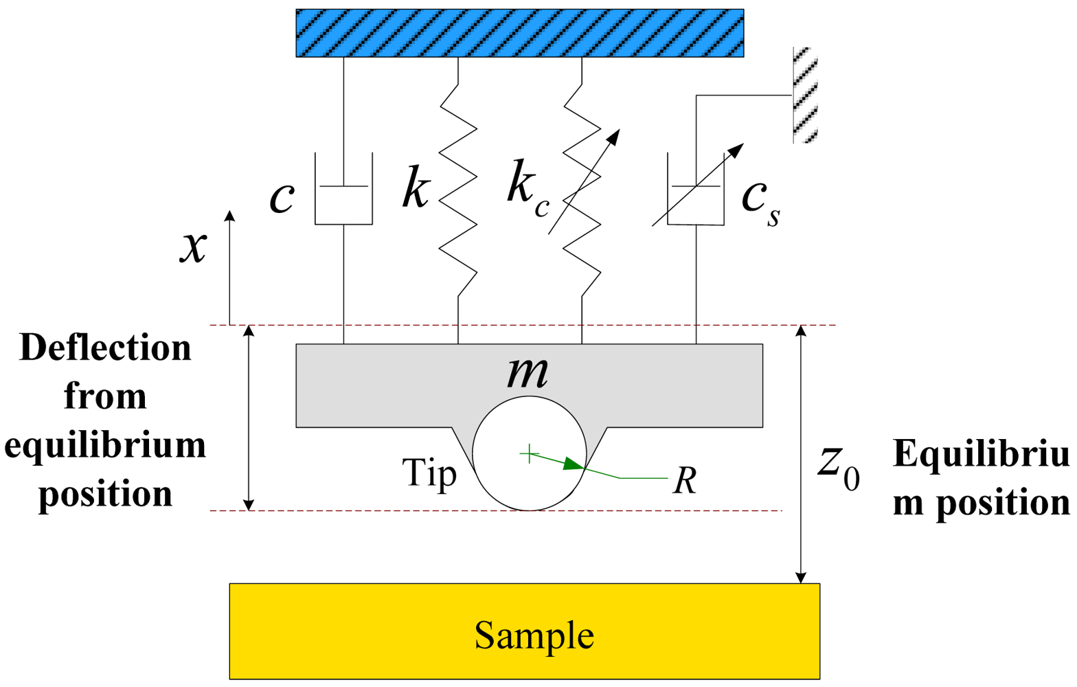
This section aims at numerically investigating the characteristics and nonlinear dynamics of a TM-AFM cantilever-sample system driven by the harmonic excitation. The general properties of the cantilever and interaction properties with the respective sample are referred to [
9], are listed in
Table 1. The 4th order Runge-Kutta method is used to integrate the set of
Equation (23). A small integration step (2π/200) has to be chosen to ensure a stable solution and to avoid the numerical divergence at the points where derivatives of
FLJ and
Fs are discontinuous. The effects of system parameters on the dynamic behavior of the cantilever vibrating system are investigated by using the bifurcation diagram, Poincaré maps, largest Lyapunov exponent, phase portraits, time histories and amplitude spectrum.
4.1. Effect of External Forcing Term Γ
The external forcing term is one of the most important parameters affecting the dynamic characteristics of the TM-AFM tip-sample system.
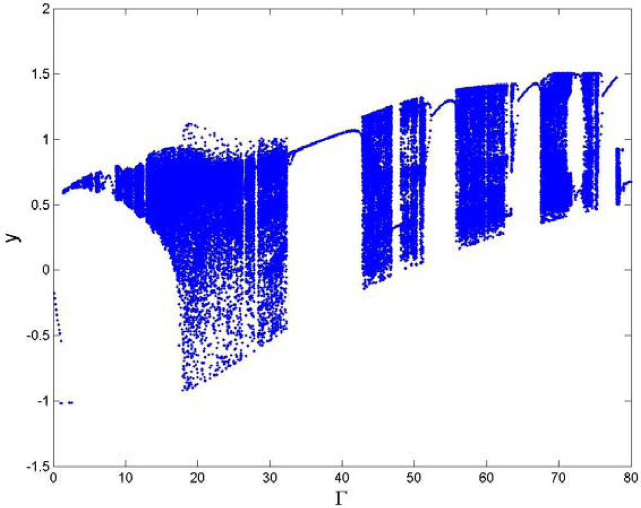
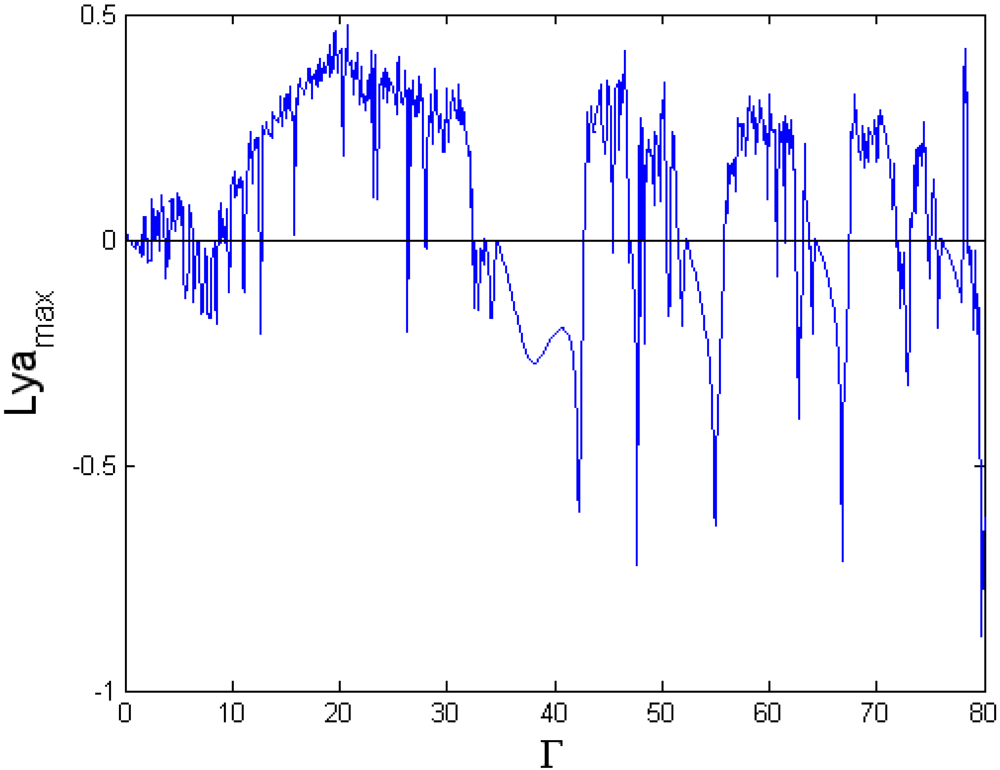
Figure 3 and
Figure 4 show the bifurcation diagram and largest Lyapunov exponent map of the dynamic system where the amplitude of the external excitation is the control parameter and the small perturbation
ε = 0.1 is added.
It can be seen from
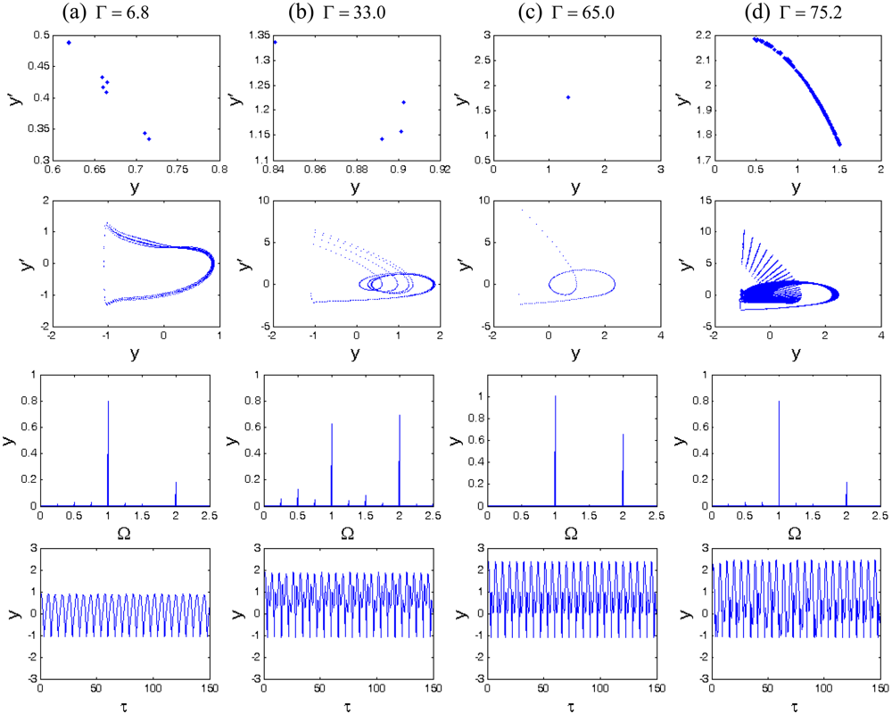
Figure 3 that the system responses contain periodic and chaotic motions alternately at the interval of 0 < Γ< 80. When Γ = 6.8, the vibration amplitude of the cantilever is small, the motion is synchronous with period-eight (P-8), and eight points are correspondingly displayed in the Poincaré map, as shown in
Figure 5(a). With the increase of the amplitude of the forcing term Γ, the motion becomes synchronous with period-two (P-2) at Γ = 33.0, as illustrated in
Figure 5(b). Moreover, the period-1 motion with only one isolated point in Poincaré map and one circle in phase portrait can be observed at Γ = 65.0 in
Figure 5(c), and the corresponding largest Lyapunov exponent becomes negative, according to
Figure 4. At Γ = 75.2, the chaos is shown in
Figure 5(d), the strange attractor has a fractal structure in Poincaré map, and it can be found in
Figure 4 that the corresponding largest Lyapunov exponent is positive. Therefore, as the amplitude of the forcing term increases, the changes of the system responses are very complex, with alternative periodic and chaotic motions.
4.2. Effect of Squeeze Film Damping η
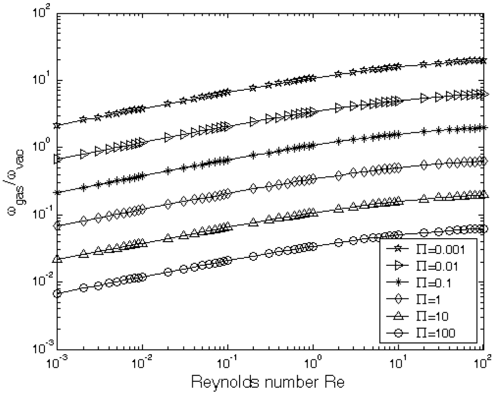
At the micro-scale, the squeeze film damping coefficient and ratio are the key parameters for the dynamic responses of the micro-devices. The larger the squeeze film damping is, the higher the noise level results. The ratio of the fundamental resonant frequency in gas to that in vacuum
ωgas/ωvac is numerically calculated from
Equation (3).
Figure 6 gives the ratio of resonant frequencies in vacuum and gas
ωgas/ωvac as a function of the Reynolds number
Re at different natural scaling parameter. ∏ It could be found that
ωgas/ωvac is increasing with the increase of Reynolds number
Re and
ωgas/ωvac decreases with the increase of the scaling parameter ∏.
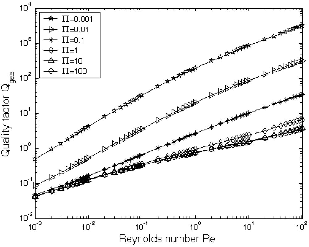
Figure 7 gives the quality factor
Qgas as a function of both natural scaling parameters,
Re and ∏, which can be obtained directly from
Equation (5). It is indicated that the quality factor
Qgas increases with the increase of the Reynolds number
Re and the decrease of the natural scaling parameter ∏. However, when the natural scaling parameter ∏ tends to be a larger value, i. e., ∏ = 10, the quality factor
Qgas has small change. For example, when ∏ changes from 10 to 100, the quality factor
Qgas has very small change, as shown in
Figure 7.
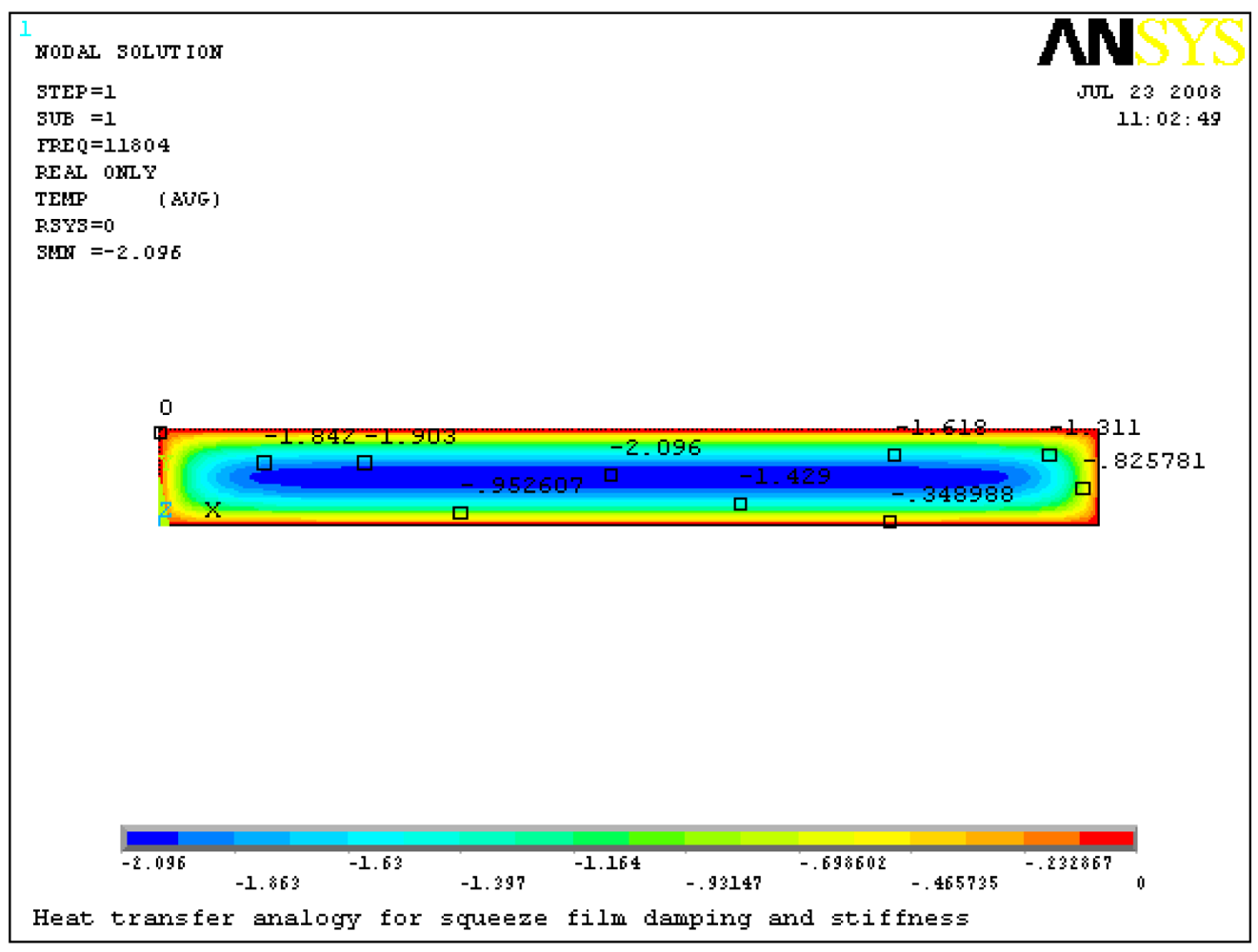
Microstructures undergoing motion transverse to a fixed plate exhibit damping effects that should be considered in the dynamics simulation. The heat transfer analogy is applied to obtain the damping and stiffness coefficients of the microstructures with PLANE 55 thermal elements in ANSYS 11.0 [
28]. The effective damping and stiffness coefficients are determined by the finite element thermal analogy approach and theoretic analyses at different operation frequencies and the results are listed in
Table 2. It can be seen that the damping coefficient decreases tardily with the increase of the operation frequency and the stiffness coefficient increases fleetly at the same time with slip and without slip. Meanwhile, the damping and stiffness coefficients with slip effect are smaller than those without slip.
Figure 8 shows the pressure distribution of the damping component with slip at the resonant frequency. The pressure distribution is approximately parabola in the directions of length and width, and the peak appears at the center of the film.
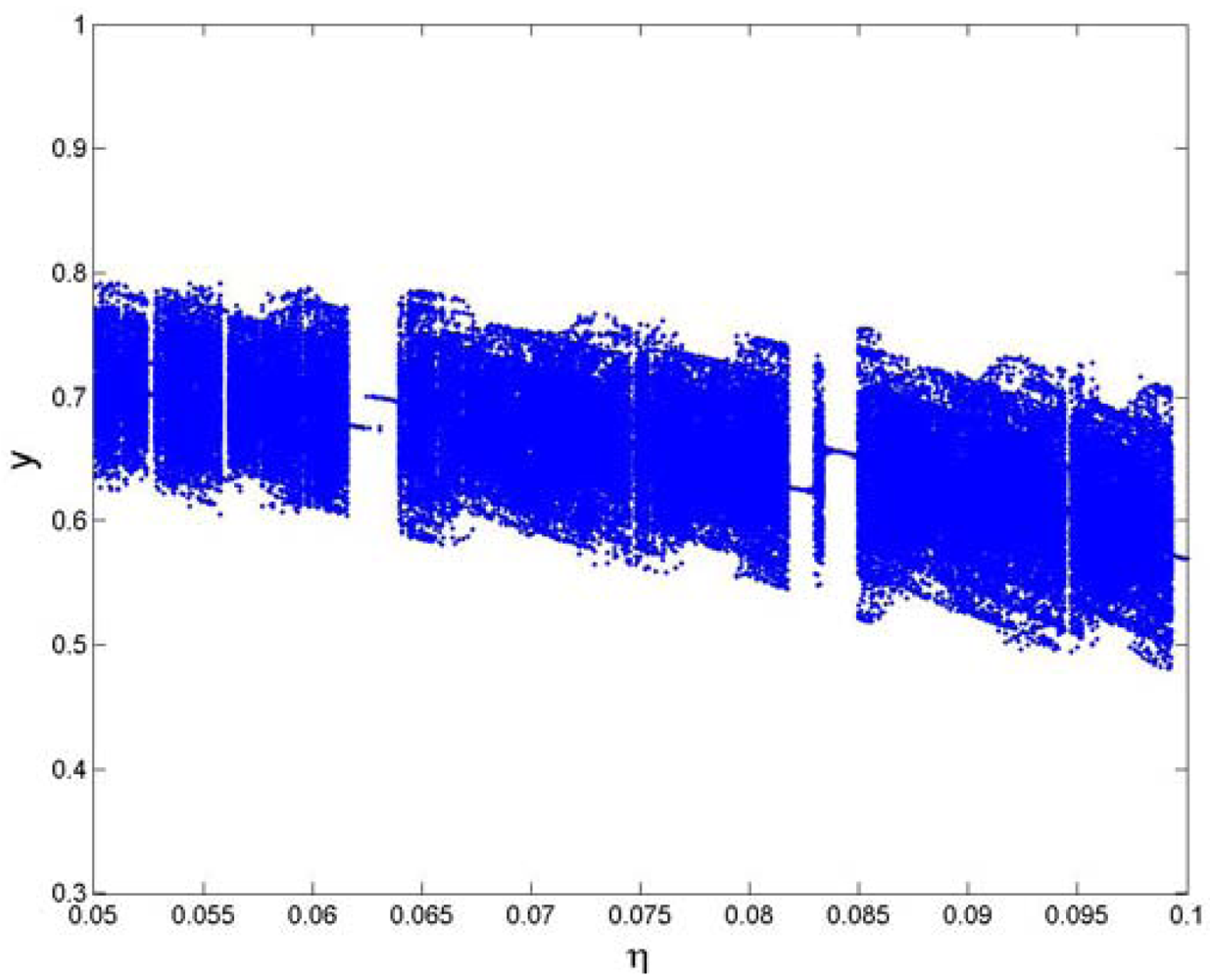
Figure 9 displays the bifurcation diagrams of squeeze film damping ratio
η in the range of 0.05 <
η < 0.1 for the coupling nonlinear dynamic system, from which it can be that the system response changes between periodic and chaotic motions alternately.
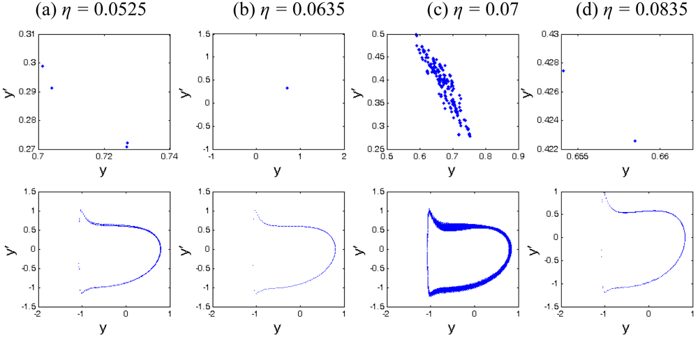
Figure 10 shows the Poincaré maps and phase plane portraits of different squeeze film damping ratio
η on the responses of the coupling system. The system response starts synchronous motion with period-4 at
η = 0.0525 (shown in
Figure 10a), and then becomes synchronous motion with period-1 at
η = 0.0635(shown in
Figure 10b), and then leaves synchronous motion with period-1 and enters chaotic motion at
η = 0.07, which can be seen in
Figure 10c. The strange attractor has a fractal structure and the corresponding largest Lyapunov exponent is positive. As indicated in
Figure 10d, with the increase of squeeze film damping ratio, the system response becomes synchronous motion with period-1 from chaotic motion. Therefore, the effect of squeeze film damping on the system response cannot be neglected for structures at the micro-scale.
4.3. Effect of material property parameter Σ
At micro-scale, the material properties of the AFM tip and sample play an important role on the surface force between them and, as a result, the dynamic response of the tip-sample system displays very rich nonlinear characteristics.
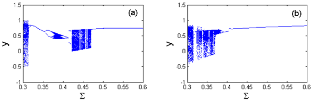
Figure 11 is the bifurcation diagram of the material property parameter
Σ for the coupling nonlinear dynamic system with different cubic stiffness ratios and squeeze film damping ratios. The system parameters are taken as follows: equilibrium parameter
α = 1.2, excitation frequency ratio Ω = 1, integration step numbers
N = 200 and the bifurcation step ΔΣ = 0.005.
Figure 11a shows the bifurcation diagram of the material property parameter in the range of 0.3 <
Σ < 0.42 with the cubic stiffness ratio
β = 0.3. The response of the coupled nonlinear system undergoes a complete process from chaotic motion through period-2, period-1, period-4 and period-8 motions to steady-state motion with period-1 by the forms of period-doubling and anti period-doubling bifurcations. At the interval of 0.42 <
Σ < 0.47, the system response alters between chaotic motion with long time and periodic motion with short time. When
Σ increases to
Σ > 0.47, the system response becomes synchronous motion with period-1. With the change of the cubic stiffness ratio of the cantilever tip from
β = 0.3 to
β = 0.5, the response of the coupled system undergoes the process of chaotic and periodic motions alternatively. It comes into period-2 motion from chaotic motion with anti period-doubling bifurcation, and then enters period-1 motion in a large range of material property parameter (
Σ > 0.39), as illustrated in
Figure 11b. In addition, it is found that the chaotic motion disappears at higher
Σ with the increase of cubic stiffness ratio (from
β = 0.3 to
β = 0.5). Therefore, with the changes of the measured samples in experimental tests, the values of
Σ vary accordingly, and as a result the response of the coupled system displays various nonlinear dynamic behaviors.
Figure 12 is the bifurcation diagram of the cubic stiffness ratio
β on the response of TM-AFM tip-sample system at the interval of 0.3 <
β < 0.6 for various combinations of squeeze film damping ratios, material and equilibrium parameters, and the bifurcation step Δ
β = 0.001. It can be observed from
Figure 12(a) that the response of the coupled system has a complete process from chaotic motion through periodic motion and chaotic motion to period-1 motion. At the interval of 0.3 <
β < 0.43, the system response enters periodic motion from chaotic motion, then it becomes chaotic motion again, and finally it comes into steady-state motion with period-1 in the range of 0.43 <
β < 0.6. With the increase of squeeze film damping
η (
η = 0.14), the system response changes noticeably and it mainly contains the periodic components, such as period-1, period-3 and period-6 motions, as illustrated in
Figure 12(c). As the equilibrium parameter
α increases, the chaotic components of the system response decrease, while the periodic components increase and contain period-2, period-4 and period-8 motions with the case of
α = 1.6, as shown in
Figure 12(d).
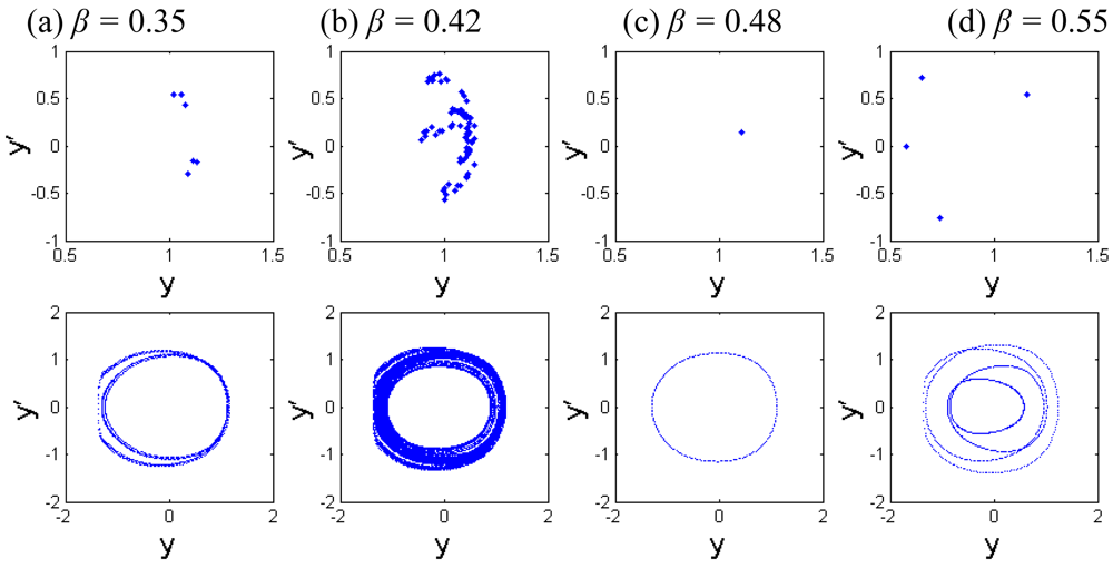
The Poincaré maps and phase portraits for different cubic stiffness ratios are displayed in
Figure 13. When the cubic stiffness ratio is small, i.e.,
β = 0.35, the exhibited motion is period-6 motion, six points and circles can be seen in the Poincaré map and phase portrait respectively from
Figure 13(a). As the cubic stiffness ratio becomes larger, the closed circle is decomposed and the points in the Poincaré map gradually scatter. At
β = 0.42, the system response comes into chaotic motion, and then the points of the attractor are decomposed again and finally converge to one point. When
β = 0.48, a synchronous motion with period-1 can be observed. Then the system response comes into period-4 motion. It is indicated that the components of chaotic motions become wider with the increase of the squeeze film damping. Material properties of the tip and sample and equilibrium coefficient ratio play very important role in the nonlinear dynamics of the coupled system.
4.4. Effect of Equilibrium Parameter α
Equilibrium coefficient ratio
α is one of the important parameters for determining the equilibrium position of the cantilever tip in AFM and it becomes the key factor to reflect the dynamic responses of the tip-sample model. The dynamic behavior of the coupled system depends on the value of
α.
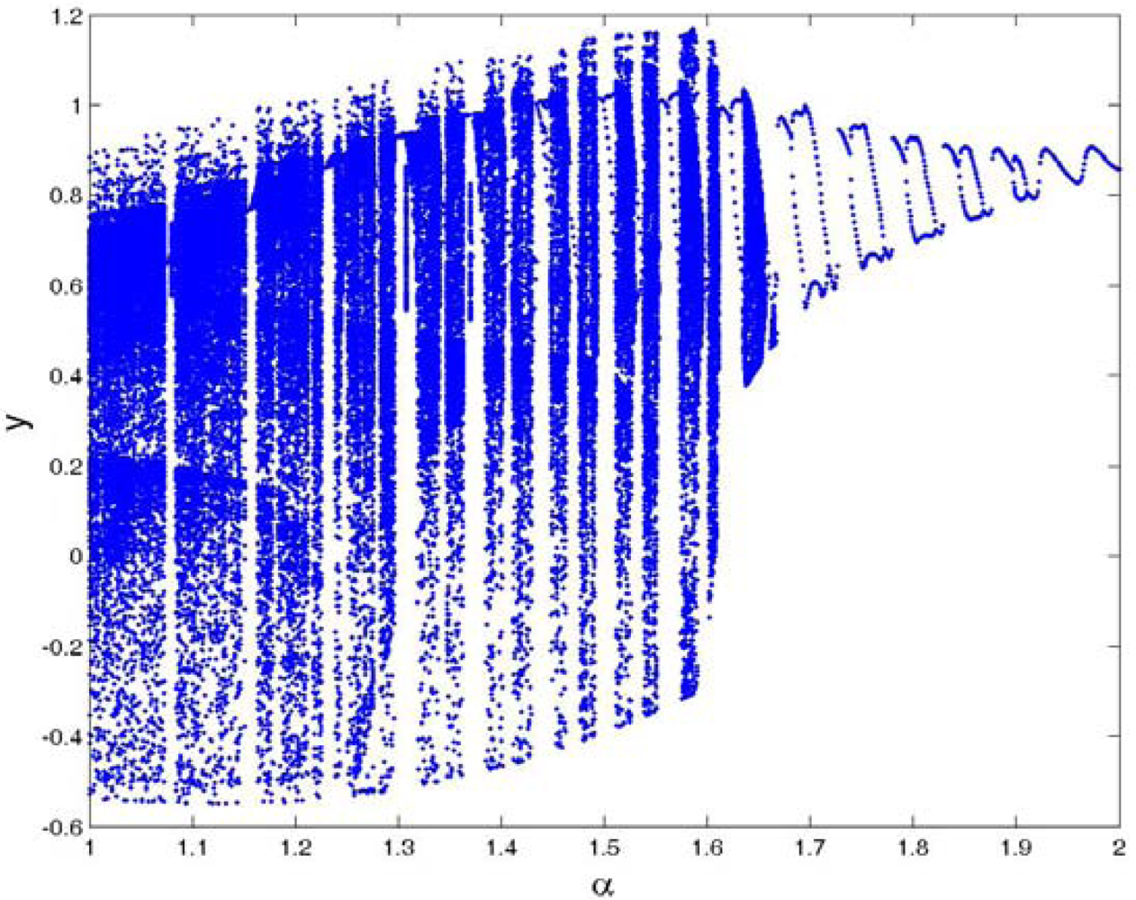
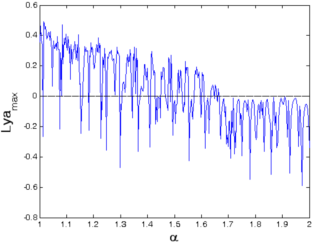
Figures 14 and
15 give the bifurcation diagram and largest Lyapunov exponent map of the dynamic system with the control parameter of the equilibrium parameter
α at Ω = 1. It can be seen from
Figure 14 that the dynamic responses are very complicated, and the components contain periodic and chaotic motions at the interval of 1<
α < 2. The corresponding largest Lyapunov exponents are alternately positive and negative, as shown in
Figure 15.
To explain the dynamic responses of the system clearly,
Figure 16 shows the local bifurcation diagram and Poincaré maps of the dynamic system at the interval of 1.6 <
α < 2. It can be found that the system responses exhibit the alternation of periodic and chaotic motions. The system response comes into steady-state synchronous motion with period-1 from chaotic motion, and enters period-2 motion from period-1 motion as the equilibrium parameter
α increases, and then becomes chaotic motion with period-doubling bifurcation. Moreover, at 1.7 <
α < 1.9, the system response changes between period-1 and period-2 motions alternately. When
α > 1.9, the system response comes into steady-state synchronous motion with period-1. These phenomena indicate that the dynamic responses of the coupled system are very complex. The cantilever tip can undergo a period-doubling cascade to possible chaos about the original equilibrium. It is demonstrated that, away from the surface, the net force on the tip is always in the downward direction and causes the tip to accelerate the sample until it passes the key point, where the repulsive force plus the spring force becomes larger than the van der Waals force, and then the tip is forced away from the sample.
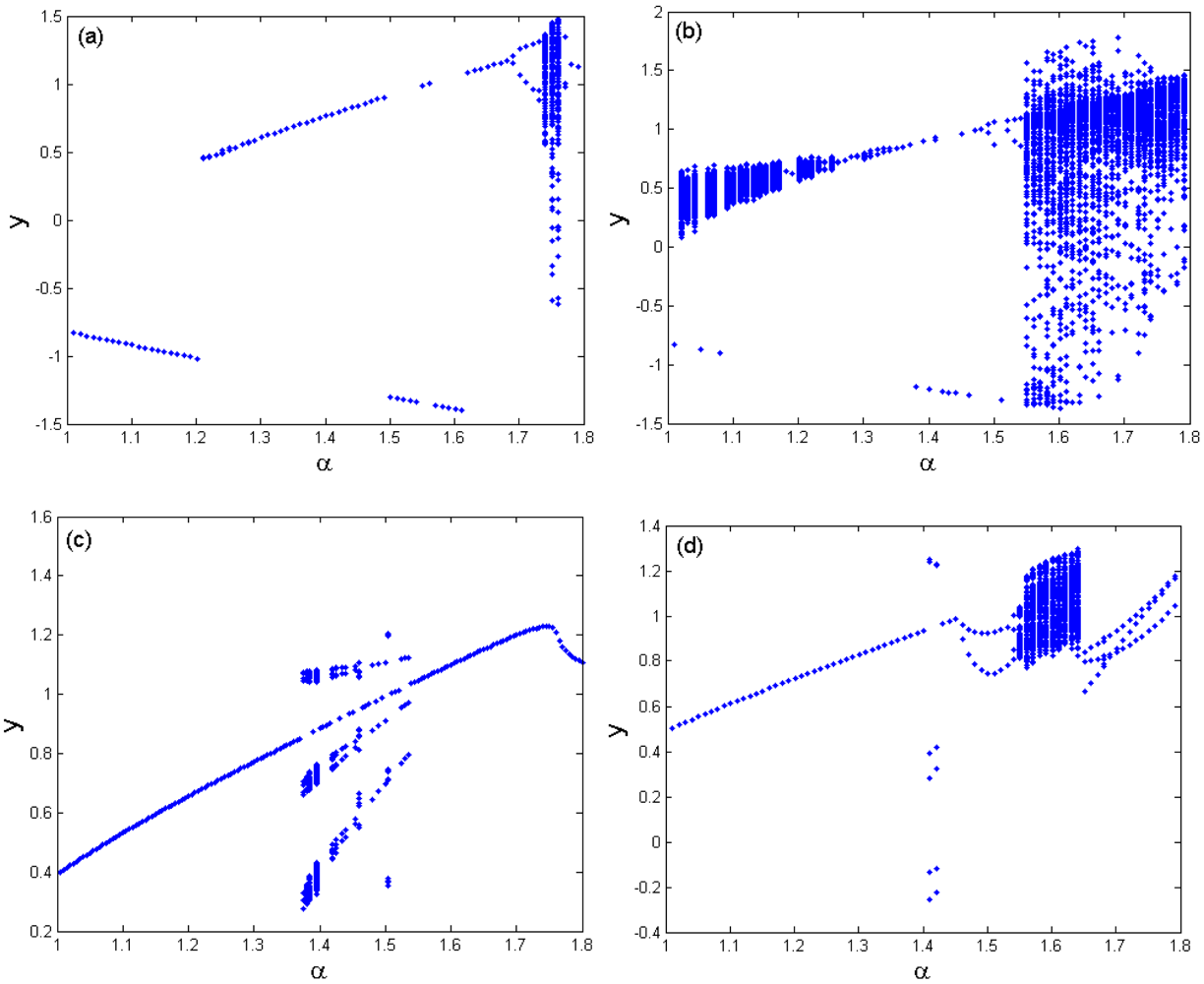
Figure 17 shows the bifurcation diagram of the equilibrium parameter
α on the response of TM-AFM tip-sample system at the interval of 1.0 <
α < 1.8, the squeeze film damping ratio is taken as
η = 0.008 and the bifurcation step is Δ
α = 0.001. It can be seen from
Figure 17(a) that the response of the coupled dynamic system comes into period-2 motion from period-1 motion and then enters chaotic motion with period-doubling bifurcation. With the increase of
α, the system responses enters period-2 motion from chaotic motion, and it subsequently becomes period-1 motion again when Σ = 0.3 and Γ = 2. As illustrated in
Figure 17(b), the response of the coupled system has a complete process from chaotic motion through periodic motion to chaotic motion with the forms of period-doubling bifurcation and anti period-doubling bifurcations at the interval of <
α < 1.8 when Σ = 0.3 and Γ = 4. With the increases of the material parameter coefficients, as shown in
Figure 17(c) and (d), the system response changes noticeably and it mainly contains the periodic components, such as period-1, period-2, period-3 and period-6 motions. Meanwhile, the chaotic components of the system response decrease and, on the contrary, the periodic components increase. In addition, the chaotic components of the system response shift to the smaller equilibrium parameter. It demonstrates that the components of chaotic motions become wider as the amplitude of external forcing term increases, and the material properties of the tip and sample and equilibrium coefficient ratio affect the nonlinear dynamics of the coupled system.
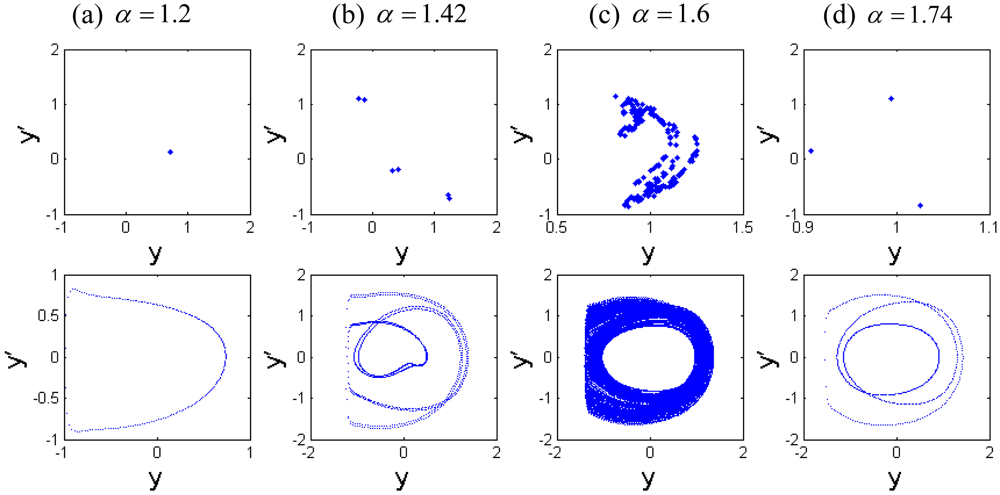
To illustrate the various motions,
Figure 18 shows the nonlinear characteristics of the coupled system with the plots of the Poincaré maps and phase portraits for different equilibrium parameters
α at different conditions. The motion of the coupled system changes between periodic and chaotic motions alternately. At
α = 1.2, the motion with period-1 represented by a point in the Poincaré maps and characterized by a close curve in phase portraits is shown in
Figure 18(a). As illustrated in
Figure 18(b), the system response comes into period-6 motion at
α = 1.42 from synchronous motion with period-1 at
α = 1.2, as displayed in
Figure 18 (a), then leaves period-6 motion and enters chaotic motion at
α = 1.6, which can be seen from
Figure 18(c). The strange attractor has a fractal structure and the corresponding largest Lyapunov exponent is positive. With the increase of the equilibrium parameter coefficient, as shown in
Figure 18(d), the system response becomes periodic motion from chaotic motion again, and one can find the period-3 motion marked by three isolated points in Poincaré map and three circles in phase portrait at
α = 1.74. It is indicated that the components of chaotic motions of the coupled system increases obviously with the increase of the amplitude of the force term. In general, the effect of equilibrium parameter on the system response should be considered for the design of the TM-AFM.


