Adapting Mobile Beacon-Assisted Localization in Wireless Sensor Networks


Abstract
:
1. Introduction
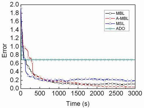
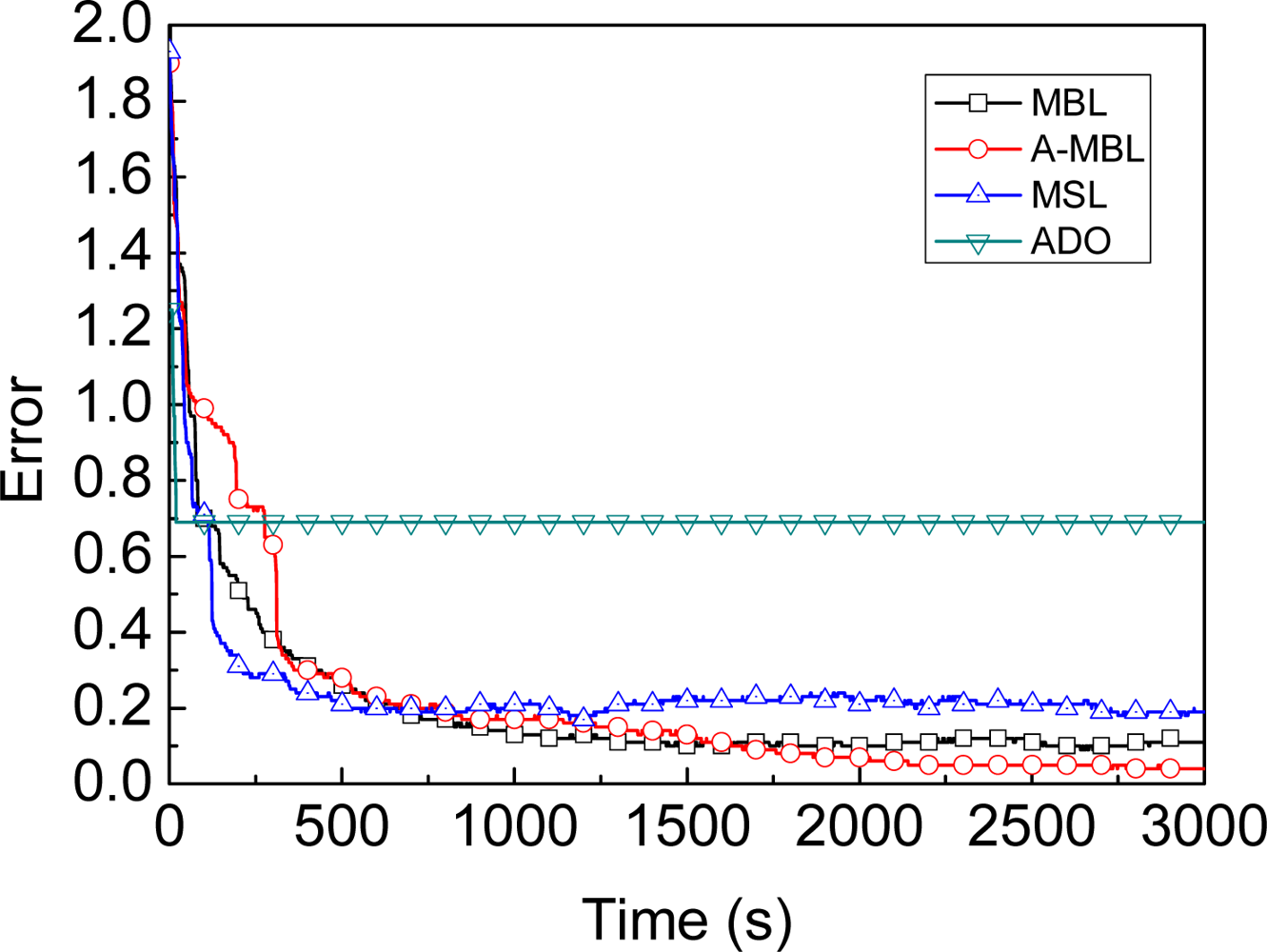
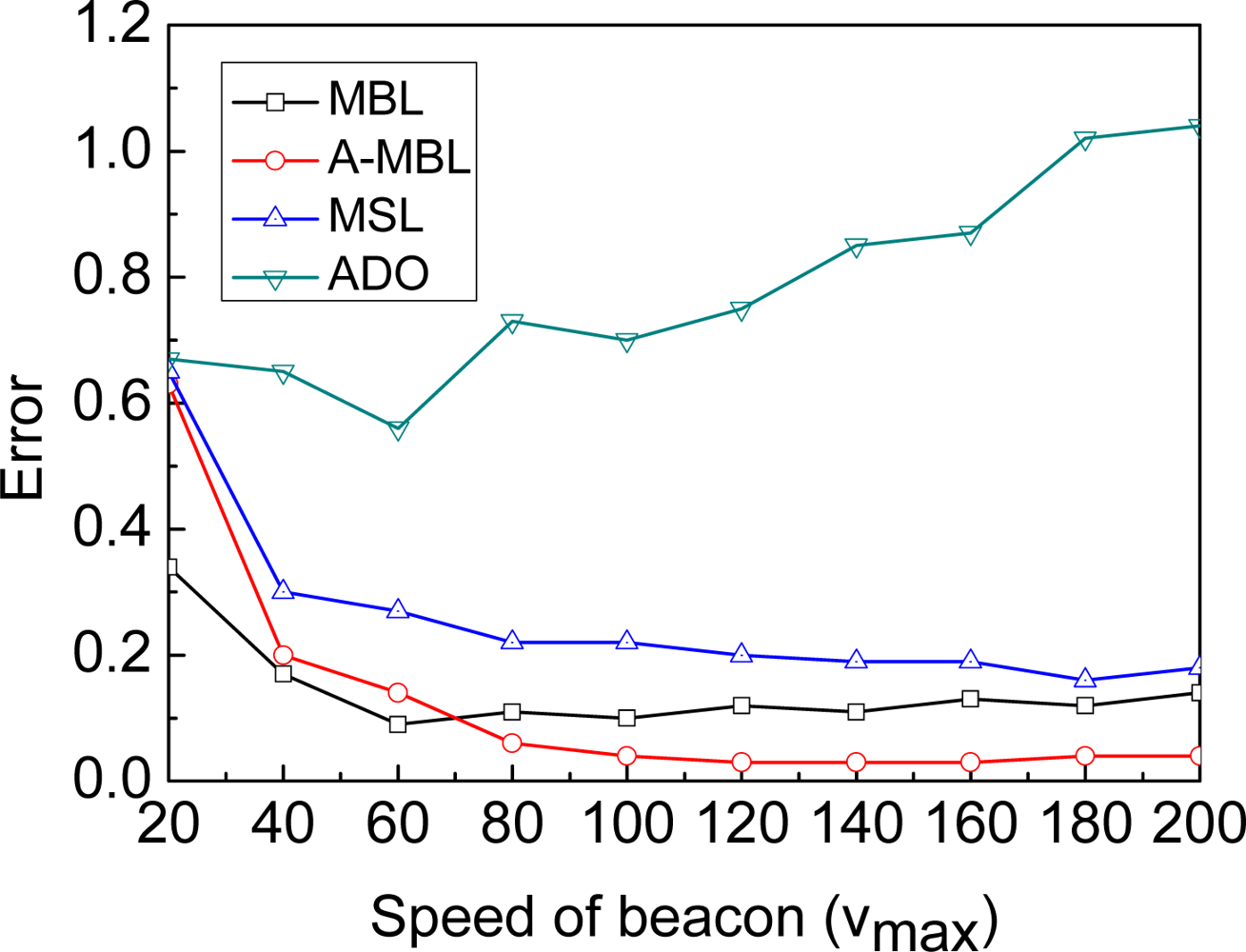
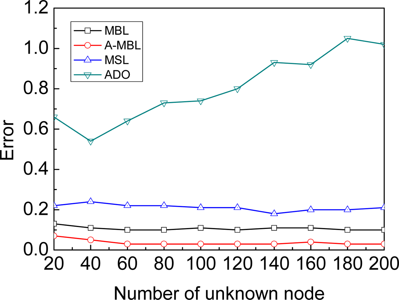
- We propose a range-free, distributed and probabilistic MBL approach. This approach outperforms both Mobile and Static sensor network Localization (MSL) and ADO when both of them use only a single mobile beacon for localization in static WSNs.
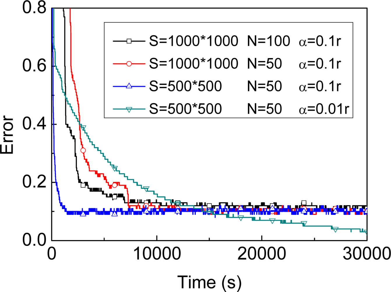
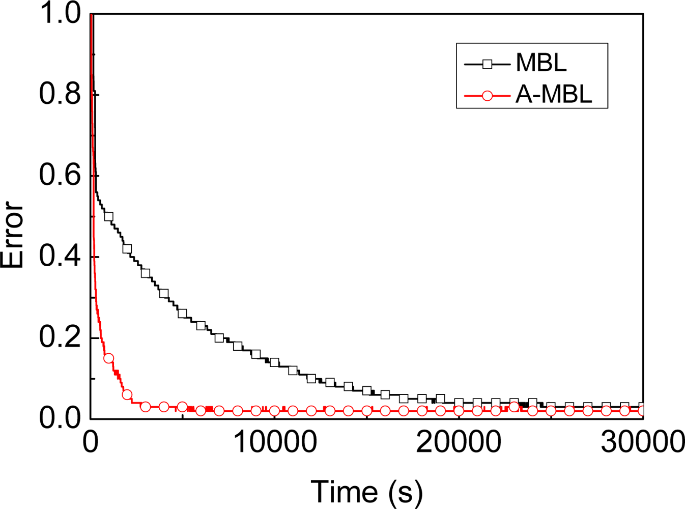
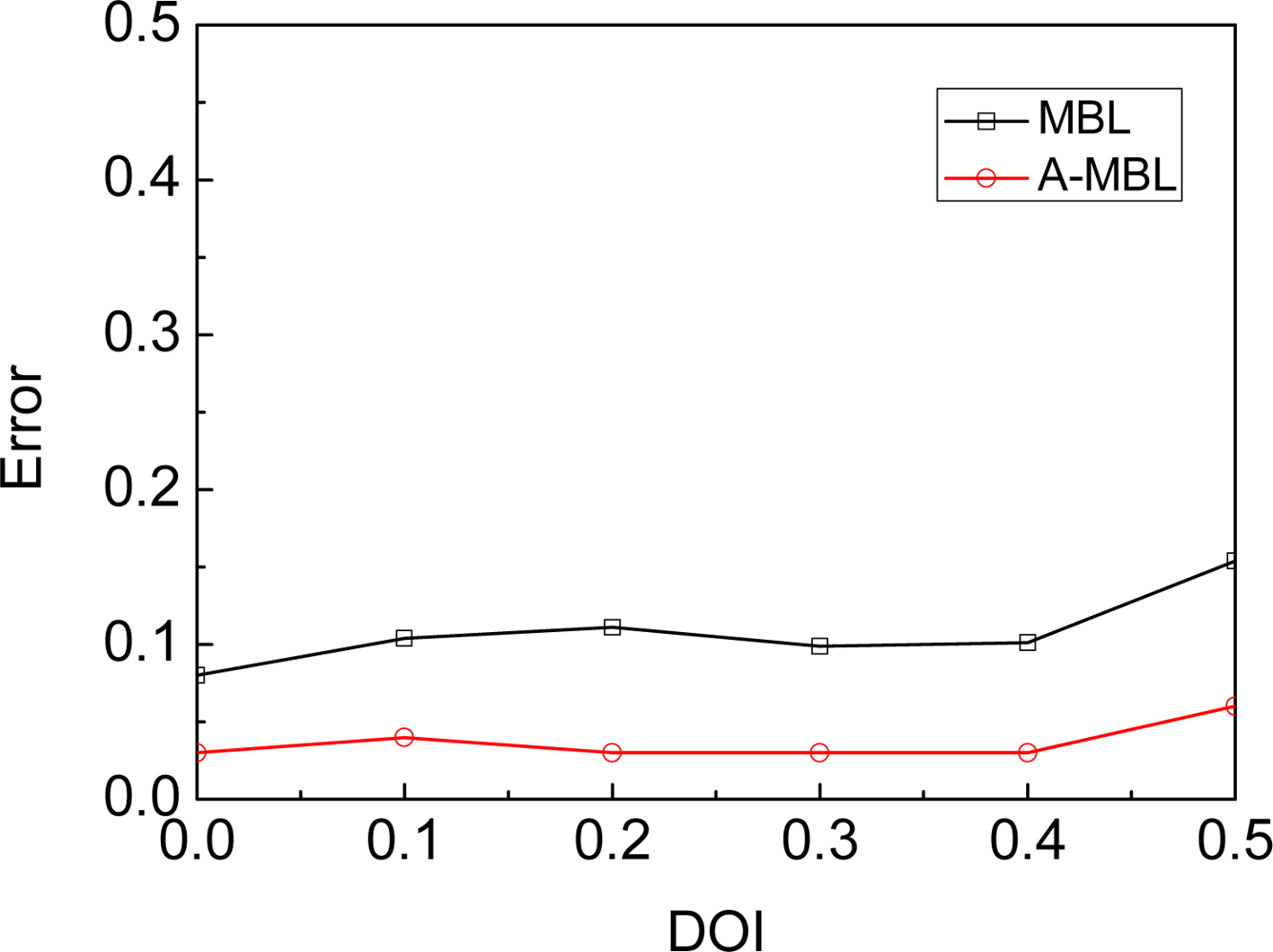
- We propose another approach based on MBL, called A-MBL, to increase the efficiency and accuracy of MBL by adapting the size of sample sets and the parameter of the dynamic model during the estimation process.
2. Description of the Problem
2.1. Mobile Beacon-assisted Localization Problem
2.2. Problem Description with Bayesian Filter
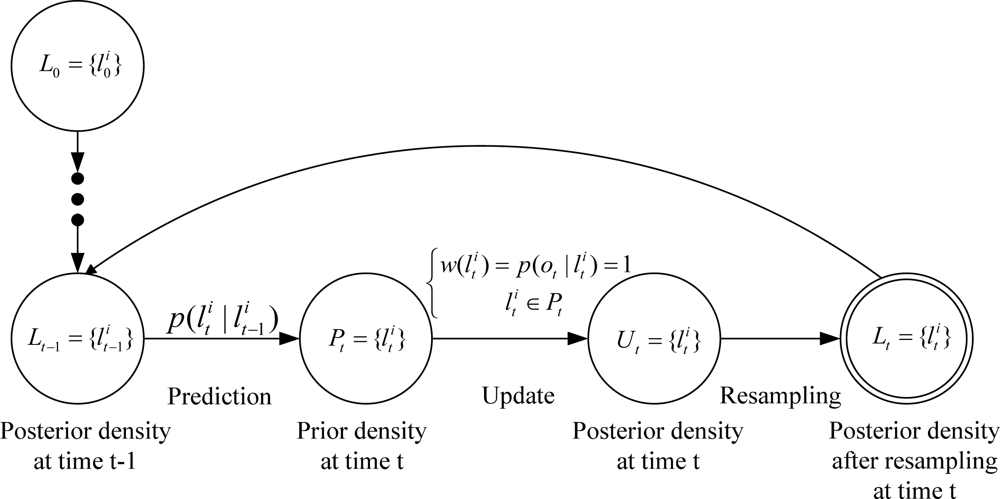
2.3. Problem Description with Particle Filter
- Initialization: N samples and weights are chosen from the initial distribution Equation (14) and the initial observation Equation (15), respectively.
- Prediction: It starts from the set of samples computed in the previous iteration, and applies the dynamic model to each sample by sampling from the density p(lt|lt−1), i.e. for each particle draw one sample from p(lt|lt−1) by:
- Update: It takes into account the observation ot. Each weight of the sample in is obtained by the importance weight Equation (13), i.e. the likelihood of given ot.
3. Mobile Beacon-Assisted Localization
3.1. MBL
- Once the unknown node is in Insider state, it gathers this observation, i.e. the filter condition of the real location R for any unknown node is:
- When the unknown node is in Arriver or Leaver state, it gathers this observation, i.e. the filter condition of the real location R for any unknown node is:where AL represents Arriver or Leaver state:

| 1: | If t=0 then |
| 2: | StateTag=FALSE |
| 3: | end if |
| 4: | filter(R)=FALSE |
| 5: | if Insider ∧ (StateTag=FALSE) then |
| 6: | filter(R)=TRUE |
| 7: | end if |
| 8: | if Outsider ∧ (StateTag=TRUE) then |
| 9: | filter(R)=TRUE |
| 10: | end if |
| 11: | if Insider then |
| 12: | StateTag=TRUE |
| 13: | else |
| 14: | StateTag=FALSE |
| 15: | end if |
3.2. A-MBL
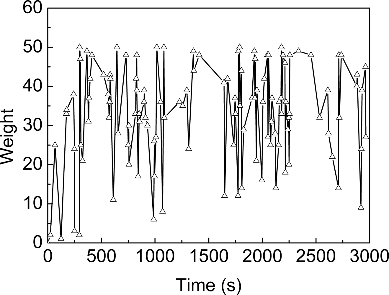
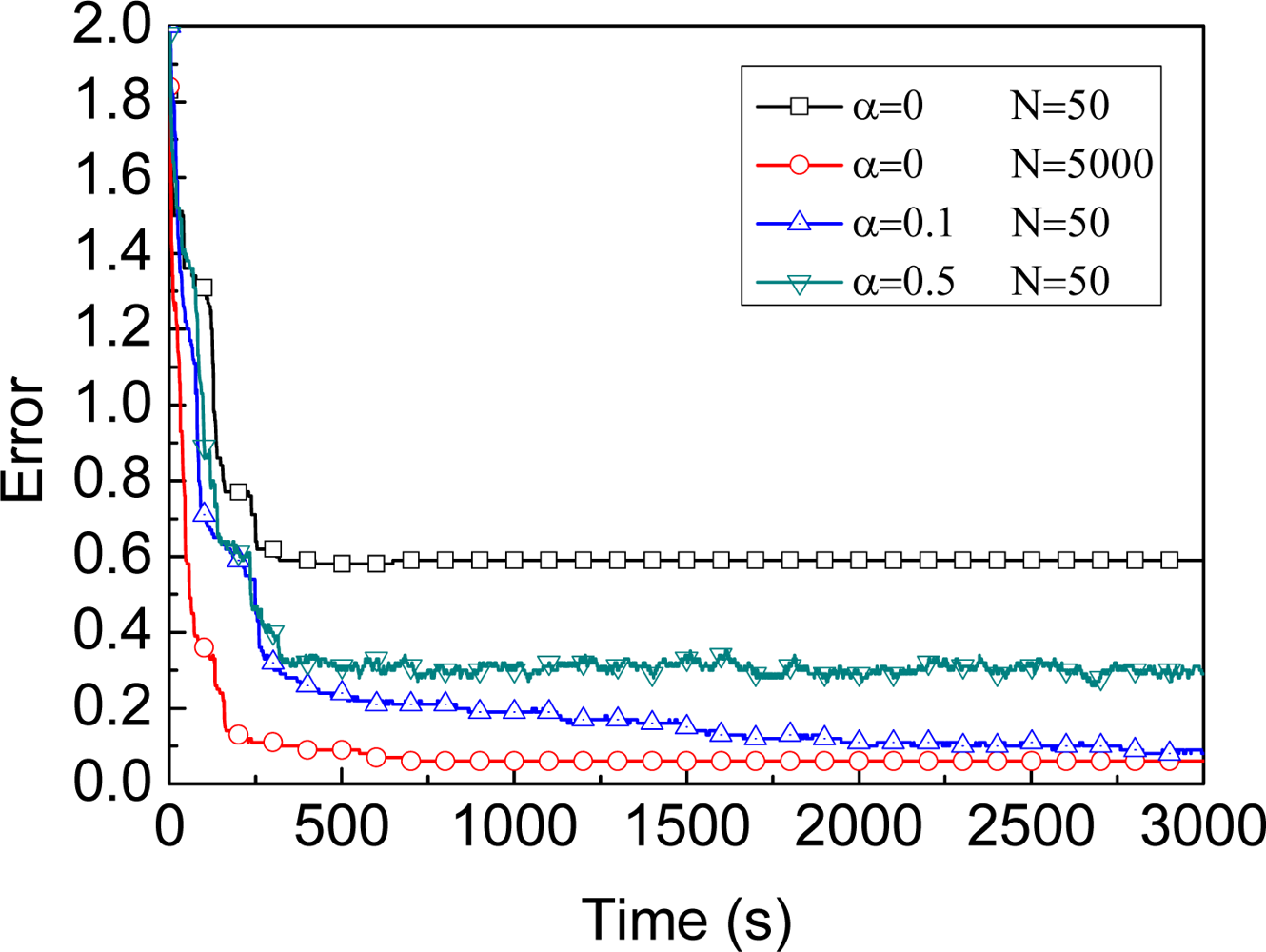
3.2.1. Number of Samples
3.2.2. Parameter α
3.2.3. Our proposed approach and implementation
| 1: | procedure ADAPTING |
| 2: | if (d(beacon,l)≤r)∧(firstContracted=FALSE) then |
| 3: | LN [kN]← InitValueFromBeacon |
| 4: | Lα[kα]←InitValueFromBeacon |
| 5: | firstContract←TRUE |
| 6: | end if |
| 7: | if (t = LN[kN].t) ∧ (kN < LN.length) then |
| 8: | Np ← N |
| 9: | N ← LN [kN].N |
| 10: | kN ← kN +1 |
| 11: | |
| 12: | |
| 13: | end if |
| 14: | if (t = Lα[kα].t) ∧ (kα < Lα.length) then |
| 15: | α ← Lα[kα].α |
| 16: | kα ← kα + 1 |
| 17: | end if |
| 18: | end procedure |
| 1: | kα ← 0 |
| 2: | kN ← 0 |
| 3: | firstContracted ← FALSE |
| 4: | for i ← 1, N do |
| 5: | INITIALIZATION |
| 6: | end for |
| 7: | for t ← 1,T do |
| 8: | for i ← 1, N do |
| 9: | |
| 10: | |
| 11: | end for |
| 12: | |
| 13: | |
| 14: | if (Neff < NT ∧ filter(l) = TRUE) then |
| 15: | |
| 16: | end if |
| 17: | ADAPTING |
| 18: | end for |
4. Evaluation
4.1. Assumption
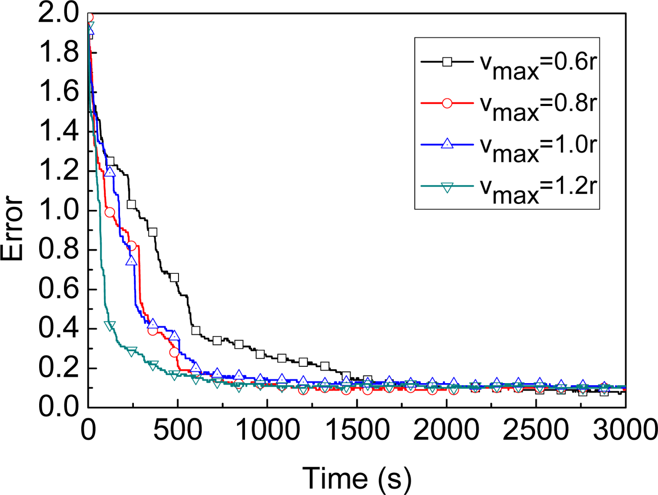
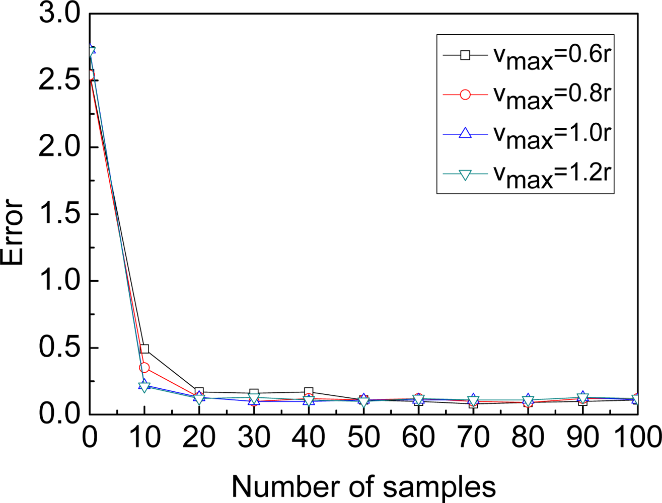
4.2. Parameters of MBL
4.3. Comparison of Different Algorithms
4.4. Irregularity
5. Related Works
6. Conclusions
Acknowledgments
References
- Volgyesi, P.; Balogh, G.; Nadas, A.; Nash, C.B.; Ledeczi, A. Shooter localization and weapon classification with soldier-wearable networked sensors. The 5th International Conference on Mobile Systems, Applications and Services, New York, NY, USA, 2007; pp. 113–126.
- Manes, G.; Fantacci, R.; Chiti, F.; Ciabatti, M.; Collodi, G.; Palma, D.D.; Manes, A. Enhanced system design solutions for wireless sensor networks applied to distributed environmental monitoring. The 32nd IEEE Conference on Local Computer Networks, Washington, DC, USA, IEEE,. 2007; pp. 807–814.
- Song, G.M.; Zhou, Y.X.; Ding, F.; Song, A.G. A Mobile Sensor Network System for Monitoring of Unfriendly Environments. Sensors 2008, 8, 7259–7274. [Google Scholar]
- Mechitov, K.; Sundresh, S.; Kwon, Y.; Agha, G. Poster abstract: cooperative tracking with binarydetection sensor networks. Proceedings of the 1st international conference on Embedded networked sensor systems, New York, NY, USA, 2003; pp. 332–333.
- Wang, X.; Wang, S.; Ma, J.J. An improved particle filter for target tracking in sensor systems. Sensors 2007, 7, 144–156. [Google Scholar]
- Szewczyk, R.; Mainwaring, A.; Polastre, J.; Anderson, J.; Culler, D. An analysis of a large scale habitat monitoring application. Proceedings of the 2nd International Conference on Embedded Networked Sensor Systems, New York, NY, USA, 2004; pp. 214–226.
- Mechitov, K.; Kim, W.; Agha, G.; Nagayama, T. High-frequency distributed sensing for structure monitoring. The First International Workshop on Networked Sensing Systems, Tokyo, Japan, 2004.
- Kwon, Y.; Agha, G. Passive localization: Large size sensor network localization based on environmental events. IEEE International Conference on Information Processing in Sensor Networks, St. Louis, Missouri, USA, 2008; pp. 3–14.
- Rudafshani, M.; Datta, S. Localization in wireless sensor networks. The 6th international conference on Information processing in sensor networks, Cambridge, Massachusetts, USA, ACM, 2007; pp. 51–60.
- Kim, K.; Lee, W. MBAL: A mobile beacon-assisted localization scheme for wireless sensor networks. The 16th International Conference on Computer Communications and Networks, Honolulu, Hawaii USA, 2007; pp. 57–62.
- Priyantha, N.B.; Balakrishnan, H.; Demaine, E.D.; Teller, S. Mobile-assisted localization in wireless sensor networks. The 24th Annual Joint Conference of the IEEE Computer and Communications Societies, Miami, USA, 2005; pp. 172–183.
- Sichitiu, M. L.; Ramadurai, V. Localization of wireless sensor networks with a mobile beacon. The First IEEE Conference on Mobile Ad-hoc and Sensor Systems, Philadelphia, USA, 2004; pp. 174–183.
- Huang, R.; Zruba, G.V. Monte carlo localization of wireless sensor networks with a single mobile beacon. Wirel. Netw 2008. [Google Scholar] [CrossRef]
- Peng, R.; Sichitiu, M.L. Robust, probabilistic, constraint-based localization for wireless sensor networks. The Second Annual IEEE Sensor and Ad Hoc Communications and Networks, Santa Clara, California, USA, 2005; pp. 541–550.
- Xiao, B.; Chen, H.K.; Zhou, S.G. A walking beacon-assisted localization in wireless sensor networks. International Conference on Communications, Glasgow, Scotland, 2007; pp. 3070–3075.
- Beeson, P.; Murarka, A.; Kuipers, B. Adapting proposal distributions for accurate, efficient mobile robot localization. IEEE International Conference on Robotics and Automation, Orlando, Florida, USA, 2006; pp. 49–55.
- Fox, D. Adapting the sample size in particle filters through KLD-sampling. Int. J. Rob. Res 2003, 22, 985–1003. [Google Scholar]
- Arulampalam, S.; Maskell, S.; Gordon, N. A tutorial on particle filters for online nonlinear/non-gaussian bayesian tracking. IEEE Trans. Signal Process 2002, 50, 174–188. [Google Scholar]
- Hu, L.; Evans, D. Localization for mobile sensor networks. The 10th Annual International Conference on Mobile Computing and Networking, New York, NY, USA, 2004; pp. 45–57.
- Kitagawa, G. Monte carlo filter and smoother for non-gaussian nonlinear state space models. J. Comput. Graph. Stat 1996, 5, 1–25. [Google Scholar]
- Fox, D.; Burgard, W.; Dellaert, F. Monte carlo localization: Efficient position estimation for mobile robots. The Sixteenth National Conference on Artificial Intelligence, Orlando, Florida, USA, 1999; pp. 343–349.
- Caballero, F.; Merino, L.; Maza, I.; Ollero, A. A Particle Filtering method for Wireless Sensor Network Localization with an Aerial Robot Beacon. IEEE International Conference on Robotics and Automation, Pasadena, CA, USA; 2008; pp. 596–601. [Google Scholar]
- Marinakis, D.; Meger, D.; Rekleitis, I.; Dudek, G. Hybrid Inference for Sensor Network Localization using a Mobile Robot. Proceedings of the Twenty-Second AAAI Conference on Artificial Intelligence, Vancouver, British Columbia, Canada; 2007; pp. 1089–1094. [Google Scholar]
- Ihler, A.T.; Fisher, J.W.; Moses, R.L.; Willsky, A.S. Nonparametric Belief Propagation for Self-Localization of Sensor Networks. IEEE J. Sel. Area Comm 2005, 23, 809–819. [Google Scholar]
- Li, M.; Liu, Y. Rendered path: range-free localization in anisotropic sensor networks with holes. The 13th Annual ACM International Conference on Mobile Computing and Networking, Montreal, Quebec, Canada, ACM, 2007; pp. 51–62.
- Stoleru, R.; He, T.; Stankovic, J. A. Walking gps: A practical solution for localization in manually deployed wireless sensor networks. The 29th Annual IEEE International Conference on Local Computer Networks, Tampa, FL, USA, 2004; pp. 480–489.
- Coates, M. Distributed Particle Filters for Sensor Networks. Third International Symposium on Information Processing in Sensor Networks, Berkeley, CA, USA, 2004; pp. 99–107.


| ID | Time | N |
|---|---|---|
| 1 | 0 | 50 |
| 2 | 2,000 | 20 |
| ID | Time | Alpha |
|---|---|---|
| 1 | 0 | 0.1 |
| 2 | 1,500 | 0.01 |
© 2009 by the authors; licensee MDPI, Basel, Switzerland This article is an open access article distributed under the terms and conditions of the Creative Commons Attribution license (http://creativecommons.org/licenses/by/3.0/).
Share and Cite
Teng, G.; Zheng, K.; Dong, W. Adapting Mobile Beacon-Assisted Localization in Wireless Sensor Networks. Sensors 2009, 9, 2760-2779. https://doi.org/10.3390/s90402760
Teng G, Zheng K, Dong W. Adapting Mobile Beacon-Assisted Localization in Wireless Sensor Networks. Sensors. 2009; 9(4):2760-2779. https://doi.org/10.3390/s90402760
Chicago/Turabian StyleTeng, Guodong, Kougen Zheng, and Wei Dong. 2009. "Adapting Mobile Beacon-Assisted Localization in Wireless Sensor Networks" Sensors 9, no. 4: 2760-2779. https://doi.org/10.3390/s90402760