Energy Efficient Sensor Scheduling with a Mobile Sink Node for the Target Tracking Application

Abstract
:1. Introduction
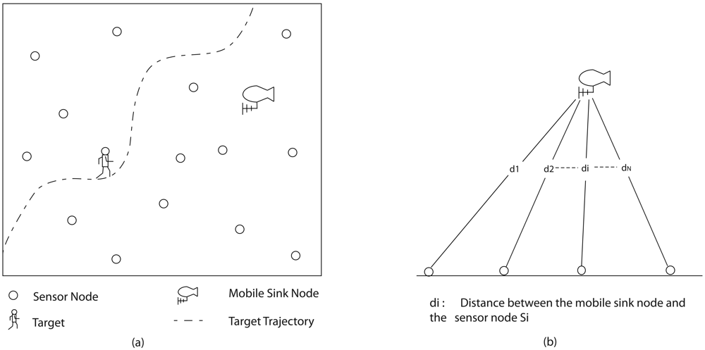
2. Problem description and Models
2.1. Sensor Model
2.2. Tracking Quality and Measurement availability
 {Xk} and its error covariance Pk∣k =
{(Xk − ξk∣k) (Xk − ξk∣k)′} at time step k are given by:
{Xk} and its error covariance Pk∣k =
{(Xk − ξk∣k) (Xk − ξk∣k)′} at time step k are given by:
3. Sensor Management with Mobile Sink Node
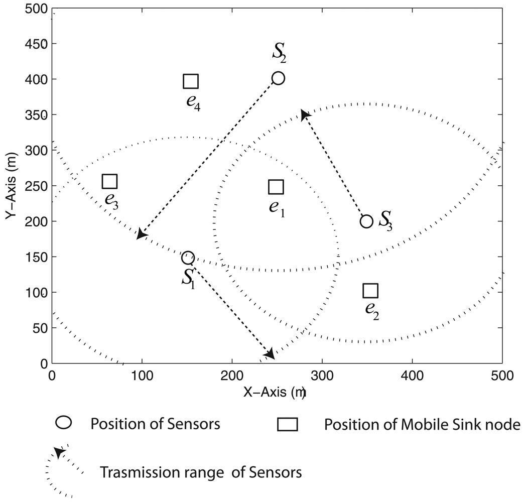
- The position of the target belongs to a known region Ωk at time step k and the sensor set {S1, S2, …, SNk} which covers the region Ωk is known a priori
- Only a single sensor node can be active mode at any time step.
- A sensor node can not be activated during the active period ti of the previously activated sensor node Si.
- The transmission range of the activated sensor node Si is set at only if ‖Li − Mk‖ > ri otherwise it remains at default range ri.
- is selected in such a way that the mobile sink node is always within the range. Thus, ‖Li − Mk‖ < and ∀ k.
3.1. Position of the mobile sink node is known
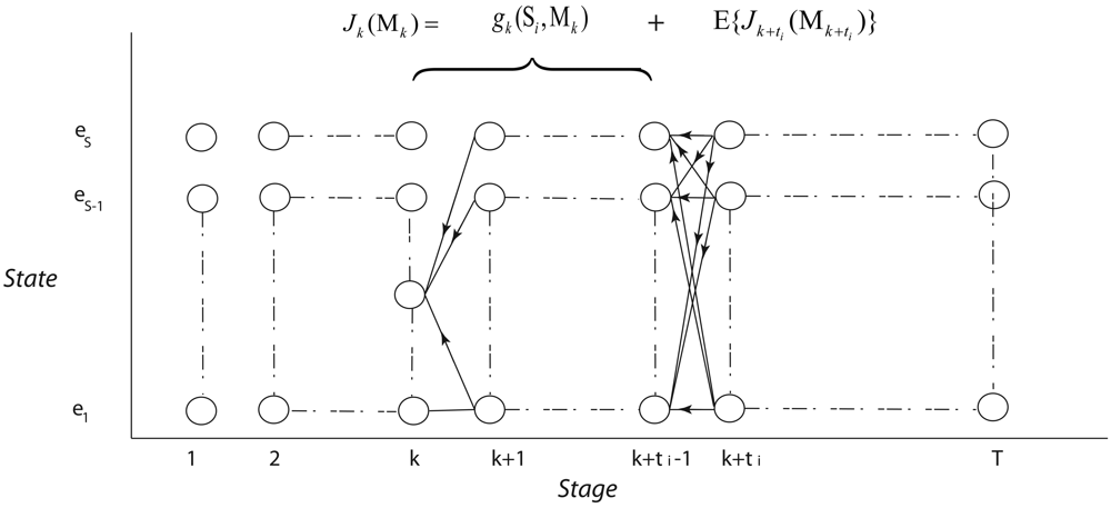
a. Dynamic Programming Approach
b. Rollout Approach
- Step1: At k = 1, update {S1, S2, …, SN1} and calculate g1(Si) + J1+ti(M1+ti), ∀ Si ∈ {S1, S2, …, SN1}. Here, J1+ti(M1+ti) is solved by the base heuristic method.
- Step 2: Choose the sensor node which minimizes g1(i) + J1+ti(M1+ti).
- Step 3: At time k, update {S1, S2, …, SN}.
- Step 4: If a sensor node Sj is in active mode set and go to Step 3 with replace k by k + 1, else go to Step 5.
- Step 5: Calculate gk(Si) + Jk+ti (Mk+ti) for all ∀ Si ∈ {1, 2, .., Nk} and Jk+ti(Mk+ti) is solved by the base heuristic method.
- Step 6: choose the sensor node which minimizes gk(Si) + Jk+ti(Mk+ti).
- Step 7: If k > T go to Step 8, else go to Step 3, replacing k with k + 1.
- Step 8: The sub-optimal sensor node sequence is given by .
3.2. Position of the mobile sink node is partially known
a. Stochastic Dynamic Programming Approach
b. One-step-look-ahead method
4. Results and Discussions
4.1. Parameter Settings for the Sensor Network
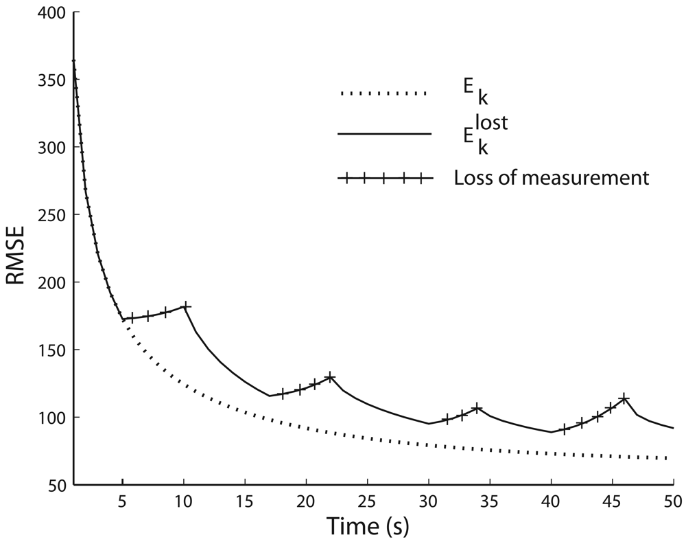
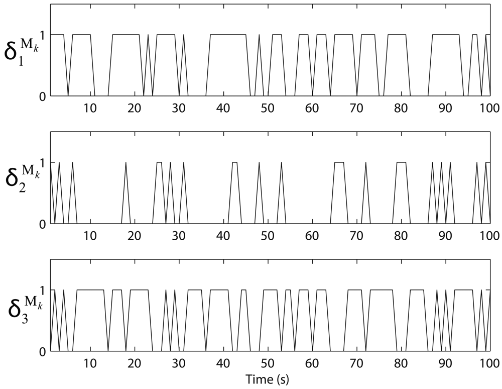
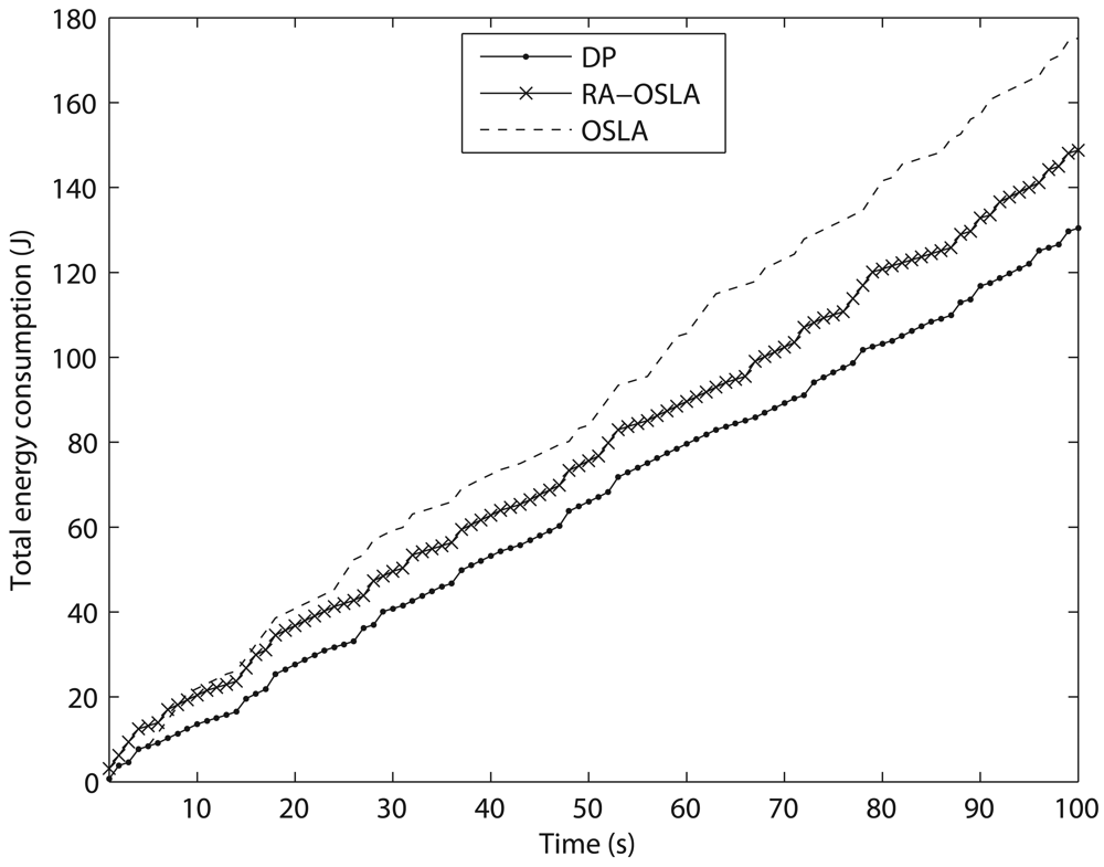
4.2. Sensor management with known mobile sink node's path
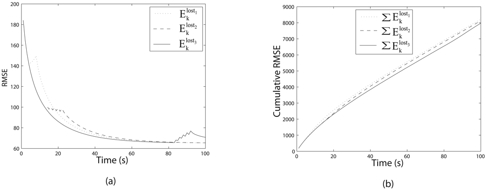
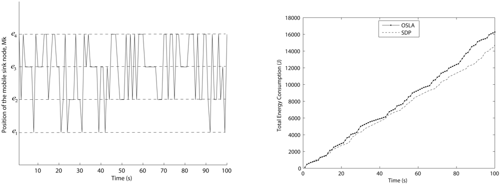
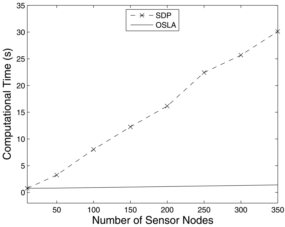
4.3. Sensor management with partially known mobile sink node's path
5. Conclusion
References and Notes
- Mahfoudh, S.; Minet, P. Survey of Energy Efficient Strategies in Wireless Ad Hoc and Sensor Networks. Seventh International Conference on Networking ICN 2008; IEEE Computer Society: Washington, DC, USA, 2008. [Google Scholar]
- Tang, X.; Xu, J. Extending Network Lifetime for Precision-Constrained Data Aggregation in Wireless Sensor Networks. 25th IEEE International Conference on Computer Communications IN-FOCOM 2006, Barcelona, Spain, April 23-29, 2006; pp. 1–12.
- Chiasserini, C.-F.; Garetto, M. Modeling the performance of wireless sensor networks. Twenty-third Annual Joint Conference of the IEEE Computer and Communications Societies INFOCOM 2004, Hong Kong, China, November 22, 2004.
- Akyildiz, I.F.; Weilian, Su; Sankarasubramaniam, Y.; Cayirci, E. A survey on sensor networks. IEEE Commun. Mag. 2002, 40, 102–114. [Google Scholar]
- Lee, D.; Kaliappan, V.K.; Chung, D.; Min, D. An energy efficient dynamic routing scheme for clustered sensor network using a ubiquitous robot, IEEE International Conference on Research, Innovation and Vision for the Future, Ho Chi Minh, July 13-17, 2008.
- Ingelrest, F.; Simplot-Ryl, D.; Stojmenovic, I. Optimal transmission radius for energy efficient broadcasting protocols in ad hoc and sensor networks. IEEE T. Parall. Distr. 2006, 17, 536–547. [Google Scholar]
- Supriyo, C.; Tim, N.; Nirvana, M.; Paul, H. A distributed and self-organizing scheduling algorithm for energy-efficient data aggregation in wireless sensor networks. ACM Trans. Sens. Netw. 2008, 4, 1–48. [Google Scholar]
- Bugra, G.; Ling, L.; Philip, S.Y. ASAP: An Adaptive Sampling Approach to Data Collection in Sensor Networks. IEEE T. Parall. Distr. 2007, 18, 1766–1783. [Google Scholar]
- Heinzelman, W.R.; Chandrakasan, A.; Balakrishnan, H. Energy-efficient communication protocol for wireless microsensor networks. Proceedings of the 33rd Annual Hawaii International Conference on System Sciences; ACM: New York, NY, USA, 2000. [Google Scholar]
- Tirta, Y.; Li, Zhiyuan; Lu, Y.; Bagchi, S. Efficient collection of sensor data in remote fields using mobile collectors. 13th International Conference on Computer Communications and Networks ICCCN; ACM: New York, NY, USA, 2004; pp. 515–519. [Google Scholar]
- Wu, Y.; Zhang, L.; Wu, Y.; Niu, Z. Interest dissemination with directional antennas for wireless sensor networks with mobile sinks. Proceedings of the 4th international conference on Embedded networked sensor systems, New York, NY, USA; 2006; pp. 99–111. [Google Scholar]
- Qin, Y.; Sun, D.; Li, N; Cen, Y. Path planning for mobile robot using the particle swarm optimization with mutation operator. Proceedings of 2004 International Conference on Machine Learning and Cybernetics, Shanghai, China, August 26-29, 2004; pp. 2473–2478.
- Verma, A.; Sawant, H.; Tan, J. Selection and Navigation of Mobile Sensor Nodes Using a Sensor Network. Third IEEE International Conference on Pervasive Computing and Communications, Kauai Island, HI, USA, March 8-12, 2005; pp. 41–50.
- Xiao, W.; Xie, L.; Lin, J.; Li, J. Multi-Sensor Scheduling for Reliable Target Tracking in Wireless Sensor Networks. 6th International Conference on ITS Telecommunications Proceedings, Chengdu, China, June 2006; pp. 41–50.
- Kreucher, C.; Hero, A.; Kastella, K.; Shapo, B. Information-based Sensor Management for Simultaneous Multitarget Tracking and Identification. Proceedings of the Thirteenth Annual Conference on Adaptive Sensor Array Processing (ASAP), Lexington, MA, June 7-8, 2005.
- Maheswararajah, S.; Halgamuge, S.; Premaratne, M. Sensor Scheduling For Target Tracking by Sub-optimal Algorithms. IEEE T. Veh. Technol. 2009. Accepted for publication. [Google Scholar]
- Williams, J.L.; Fisher, J.W.; Willsky, A.S. Approximate Dynamic Programming for Communication-Constrained Sensor Network Management. IEEE T. Signal Proces. 2007, 55, 4300–4311. [Google Scholar]
- Xue, W.; Jun-Jie, M.; Sheng, W.; Dao-Wei, B. Cluster-based Dynamic Energy Management for Collaborative Target Tracking in Wireless Sensor Networks. Sensors 2007, 7, 1193–1215. [Google Scholar]
- Hernandez, M.L.; Kirubarajan, T.; Bar-Shalom, Y. Multisensor resource deployment using posterior Cramer-Rao bounds. IEEE T. Aero. Elec. Sys. 2004, 40, 399–416. [Google Scholar]
- Chhetri, A.S.; Morrell, D.; Papandreou-Suppappola, A. Energy efficient target tracking in a sensor network using non-myopic sensor scheduling. 8th International Conference on Information Fusion, Philadelphia, USA, July 25-28, 2005; p. 8.
- Shah, H.; Morrell, D. Non-myopic sensor scheduling for a distributed sensor network, IEEE International Conference on Acoustics, Speech and Signal Processing, Las Vegas, March 30-April 4, 2008; pp. 2541–2544.
- Gupta, V.; Chung, T.; Hassibi, B.; Murray, R.M. On a Stochastic Sensor Selection Algorithm with Applications in Sensor Scheduling and Sensor Coverage. Automatica 2006, 42, 251–260. [Google Scholar]
- Tharmarasa, R.; Kirubarajan, T.; Hernandez, M.L.; Sinha, A. PCRLB-based multisensor array management for multitarget tracking. IEEE T. Aero. Elec. Sys. 2007, 43, 539–55. [Google Scholar]
- John, S.B.; Alain, B. Sensor scheduling problems. Proceedings of 27 th IEEE International Conference on Decision and Control, Austin, Texas, December 1998; pp. 2342–2345.
- Bhardwaj, M.; Chandrakasan, A.P. Bounding the lifetime of sensor networks via optimal role assignments. Twenty-First Annual Joint Conference of the IEEE Computer and Communications Societies, New York, USA, June 23-27, 2002; pp. 1587–1596.
- Gupta, V.; Chung, T.; Hassibi, B.; Murray, R.M. Sensor scheduling algorithms requiring limited computation [vehicle sonar range-finder example]. IEEE International Conference on Acoustics, Speech, and Signal Processing, Montreal, CA, May 17-21, 2004; pp. iii-825–8.
- Tichavsky, P.; Muravchik, C.H.; Nehorai, A. Posterior Cramer-Rao bounds for discrete-time nonlinear filtering. IEEE T. Signal Proces. 1998, 46, 1386–1396. [Google Scholar]
- Krishnamurthy, V. Algorithms for optimal scheduling and management of hidden Markov model sensors. IEEE T. Signal Proces. 2002, 50, 1382–1397. [Google Scholar]
- Evans, J.; Krishnamurthy, V. Optimal sensor scheduling for Hidden Markov models. Proceedings of the 1998 IEEE International Conference on Acoustics, Speech, and Signal Processing, Seattle, WA, USA; 1998; pp. 2161–2164. [Google Scholar]
- Yaakov, B.; Thiagalingam, K.; Rong, L. Estimation with Applications to Tracking and Navigation; John Wiley & Sons, Inc.: New York, NY, USA, 2002. [Google Scholar]
- Kalman, R.E. A New Approach to Linear Filtering and Prediction Problems. Trans. ASME, J. Basic Eng. 1960, 35–45. [Google Scholar]
- Bertsekas, D.P. Dynamic Programming and Optimal Control, third edition; Volume 3, Athena Scientific, 2005. [Google Scholar]


| Sensor Node (Si) | Coordinate (Li) | Transmission Range (ri) | Active time period (ti) |
|---|---|---|---|
| S1 | (150, 150, 0)m | 200m | 5s |
| S2 | (350, 200, 0)m | 300m | 4s |
| S3 | (250, 400, 0)m | 200m | 2s |
| T (s) | OSLA (J) | RA-OSLA (J) | DP (J) |
|---|---|---|---|
| 30 | 59.0 | 48.8 | 40.8 |
| 40 | 72.4 | 62.4 | 49.6 |
| 50 | 84.0 | 74.4 | 63.2 |
| 60 | 105.6 | 89.6 | 76.8 |
| 70 | 123.2 | 101.6 | 89.2 |
| 80 | 141.6 | 118.4 | 103.2 |
| 90 | 157.2 | 130.0 | 114.8 |
| 100 | 175.2 | 148.8 | 130.0 |
| T (s) | JT with A1 | JT with A2 | ||
|---|---|---|---|---|
| OSLA (J) | SDP (J) | OSLA (J) | SDP (J) | |
| 30 | 47.80±5.48 | 42.50±5.01 | 51.33±6.26 | 46.12±5.16 |
| 40 | 64.12±6.53 | 56.61±5.77 | 67.86±7.43 | 61.50±5.92 |
| 50 | 80.24±7.36 | 70.70±6.41 | 85.19±8.56 | 77.10±6.75 |
| 60 | 96.45±7.87 | 85.14±7.05 | 101.79±8.80 | 92.67±7.27 |
| 70 | 112.55±8.89 | 99.46±7.63 | 118.97±9.27 | 107.80±8.04 |
| 80 | 128.34±8.93 | 113.26±7.98 | 136.77±9.99 | 123.38±8.48 |
| 90 | 144.87±9.64 | 127.84±8.48 | 153.43±10.91 | 138.69±9.01 |
| 100 | 160.90±10.15 | 143.27±9.05 | 170.82±11.35 | 155.74±9.65 |
6. Notes Added in Proof
- In page 5, last paragraph:Original versionwhere wk is the white Gaussian process noise with a known covariance Q and the intensity of the process noise is determined by the matrix B.Corrected versionwhere wk is the white Gaussian process noise with a known covariance Q and the intensity of the process noise is determined by the scalar quantity q.
- In page 15, Figure 5: y-axis texts are enlarged to make it more clearer.
© 2009 by the authors; licensee Molecular Diversity Preservation International, Basel, Switzerland. This article is an open access article distributed under the terms and conditions of the Creative Commons Attribution license (http://creativecommons.org/licenses/by/3.0/).
Share and Cite
Maheswararajah, S.; Halgamuge, S.; Premaratne, M. Energy Efficient Sensor Scheduling with a Mobile Sink Node for the Target Tracking Application. Sensors 2009, 9, 696-716. https://doi.org/10.3390/s90100696
Maheswararajah S, Halgamuge S, Premaratne M. Energy Efficient Sensor Scheduling with a Mobile Sink Node for the Target Tracking Application. Sensors. 2009; 9(2):696-716. https://doi.org/10.3390/s90100696
Chicago/Turabian StyleMaheswararajah, Suhinthan, Saman Halgamuge, and Malin Premaratne. 2009. "Energy Efficient Sensor Scheduling with a Mobile Sink Node for the Target Tracking Application" Sensors 9, no. 2: 696-716. https://doi.org/10.3390/s90100696