Sonar Sensor Models and Their Application to Mobile Robot Localization


Abstract
:
1. Introduction
2. The Polaroid Sensor
2.1. Overview
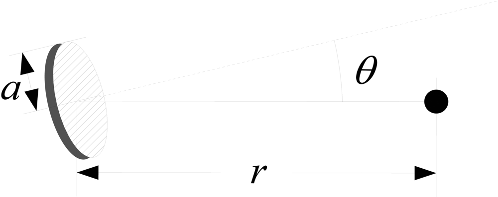
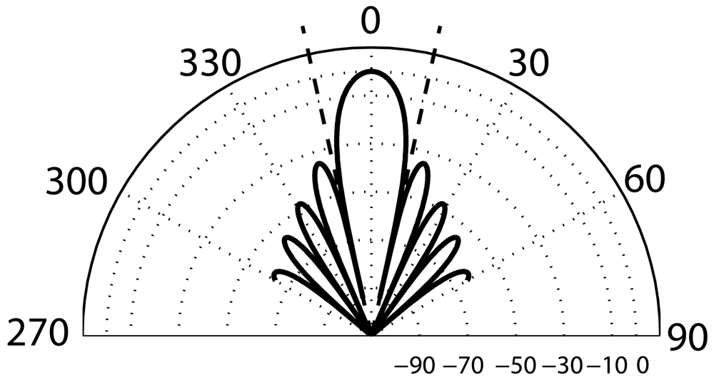
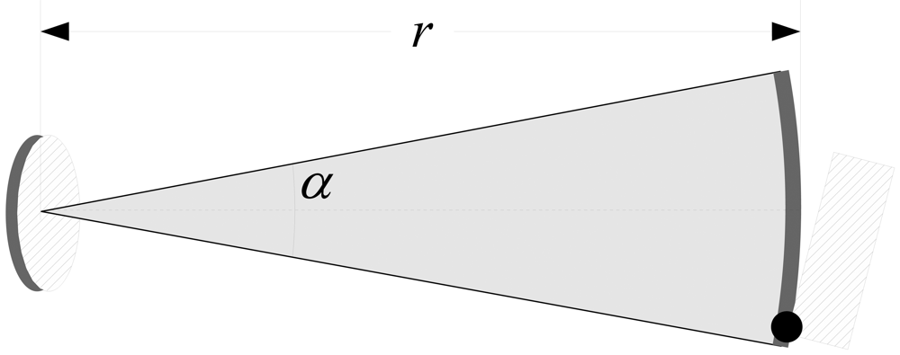
2.2. Theoretical Model
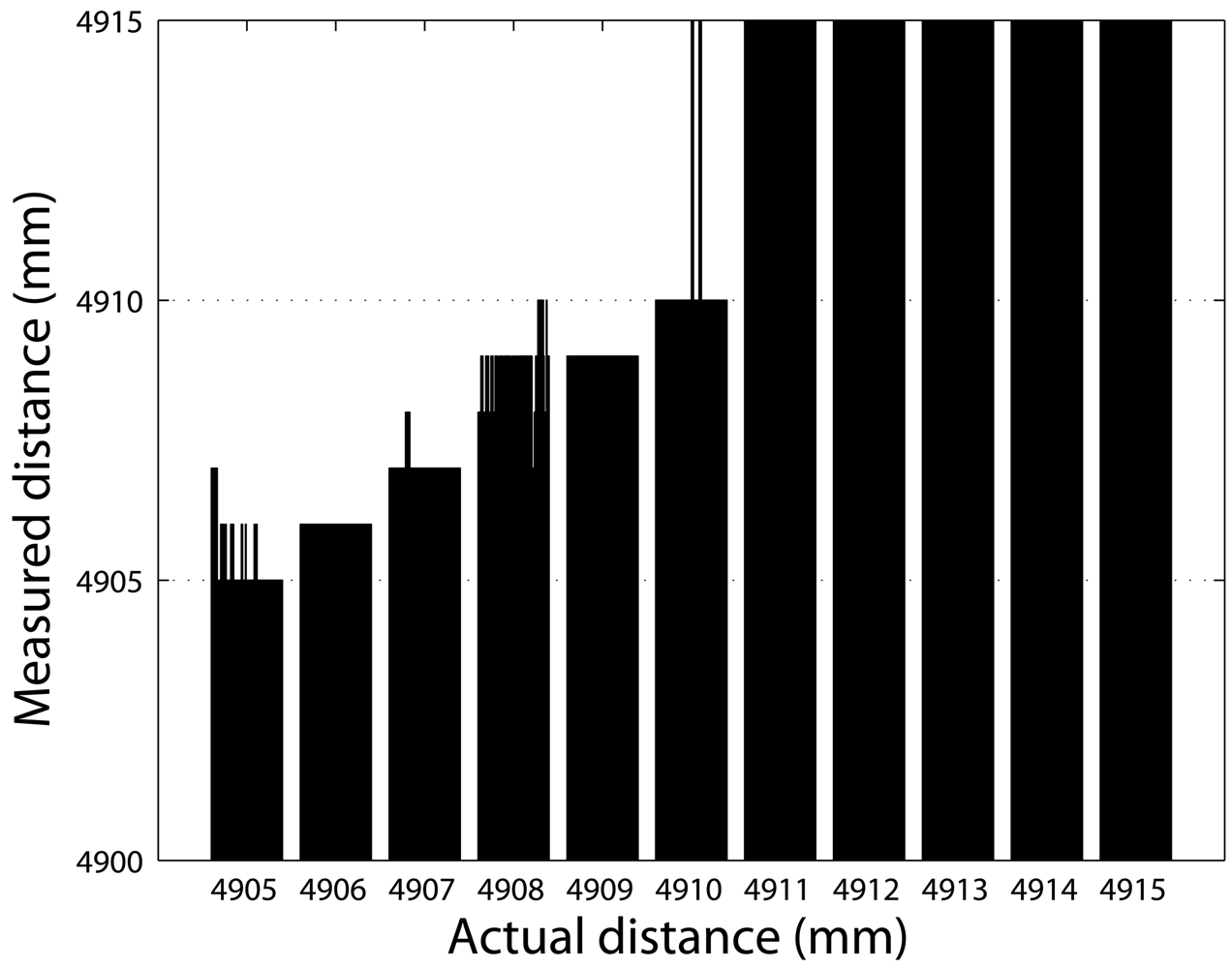
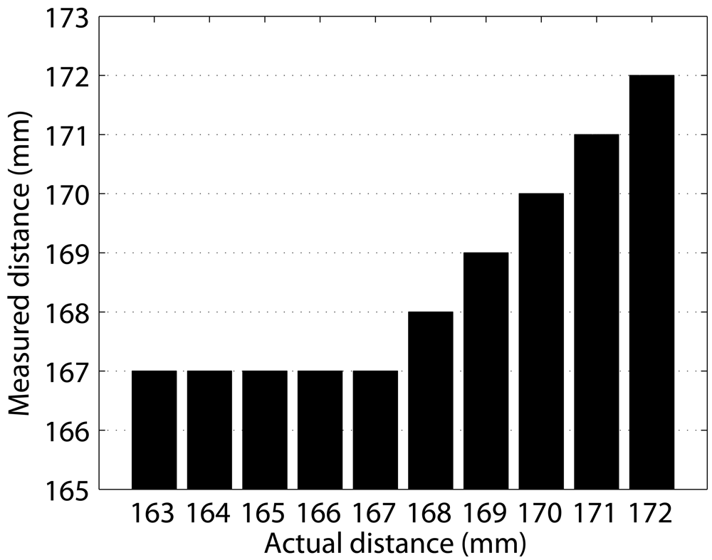
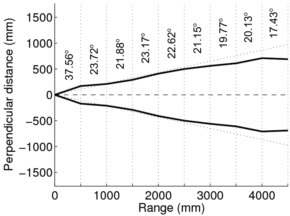
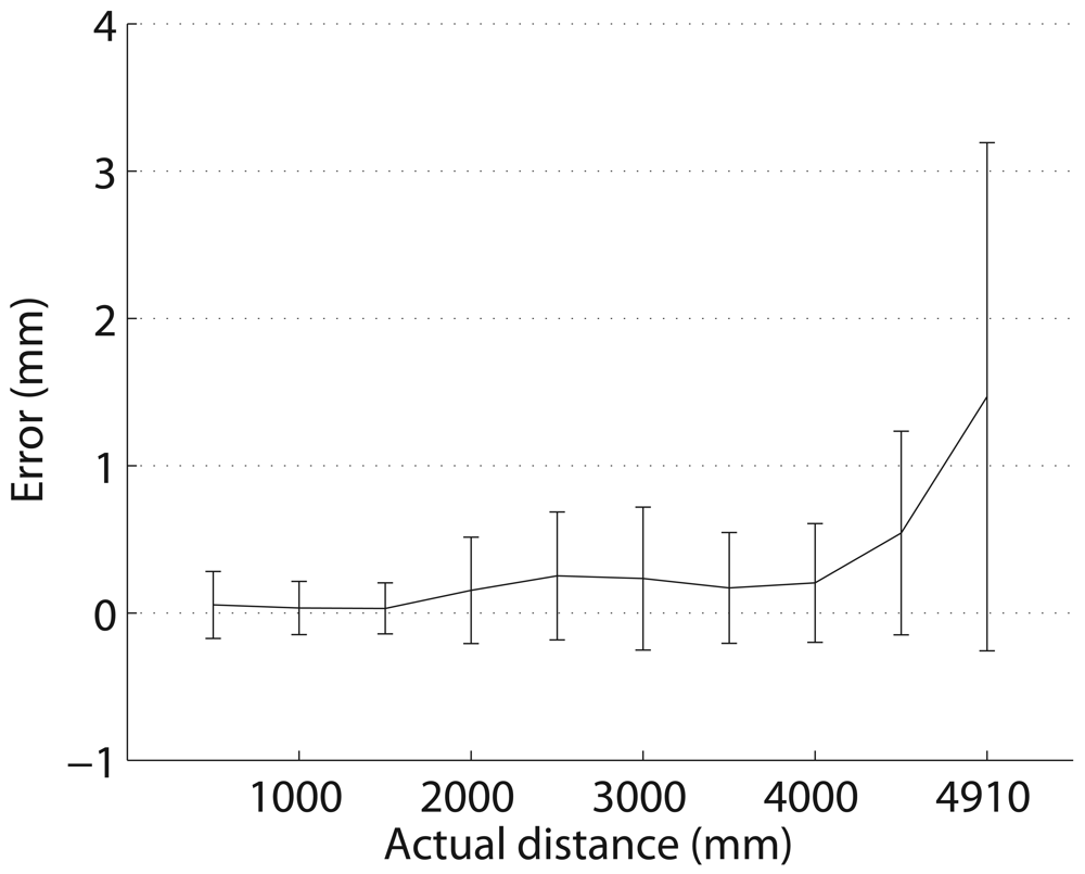
2.3. Experimental Characterization
3. The Sonar Monte Carlo Localization Approach
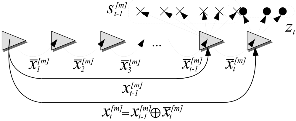
3.1. Overview and Notation
3.2. Initialization
3.3. The Particle Filter
| Algorithm 1: The Particle Filter algorithm. | |
| 1 | begin |
| 2 | for m → 1 to M do |
| 3 | |
| 4 | |
| 5 | endfor |
| 6 | for m ← 1 to M do |
| 7 | draw i with probability |
| 8 | |
| 9 | |
| 10 | |
| 11 | endfor |
| 12 | end |
4. The Measurement Model
4.1. The Probabilistic Sonar Model
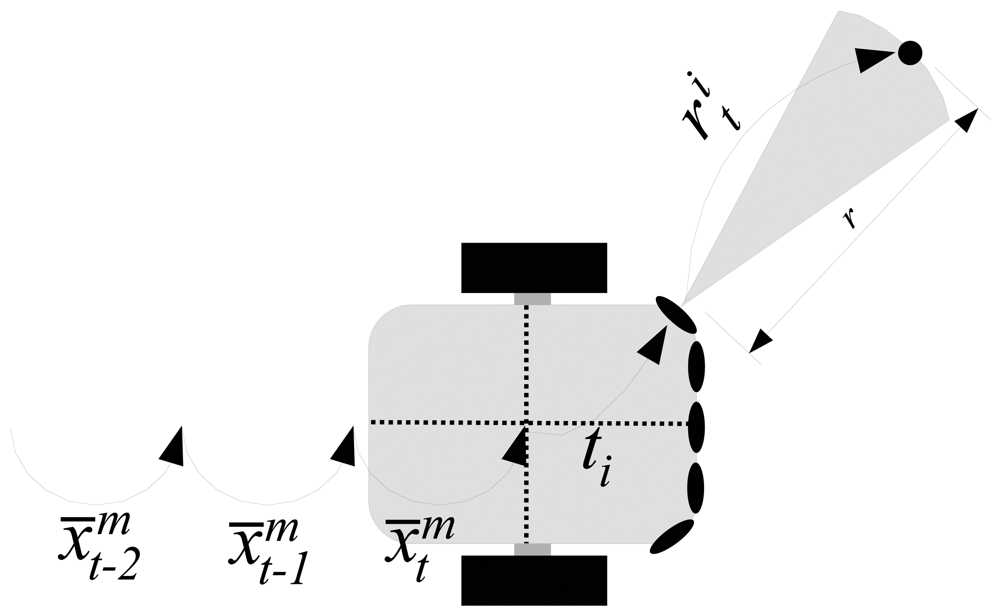
4.2. Building the Local Maps
4.3. The Probabilistic Approach
5. Experimental Results
5.1. Experimental Setup
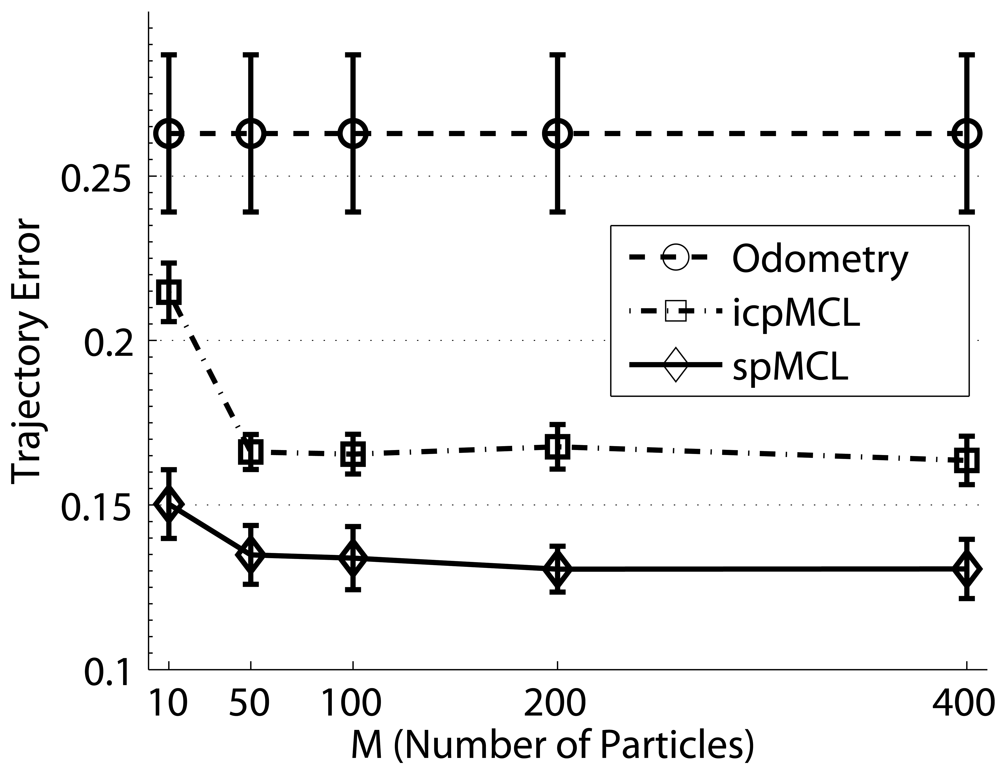
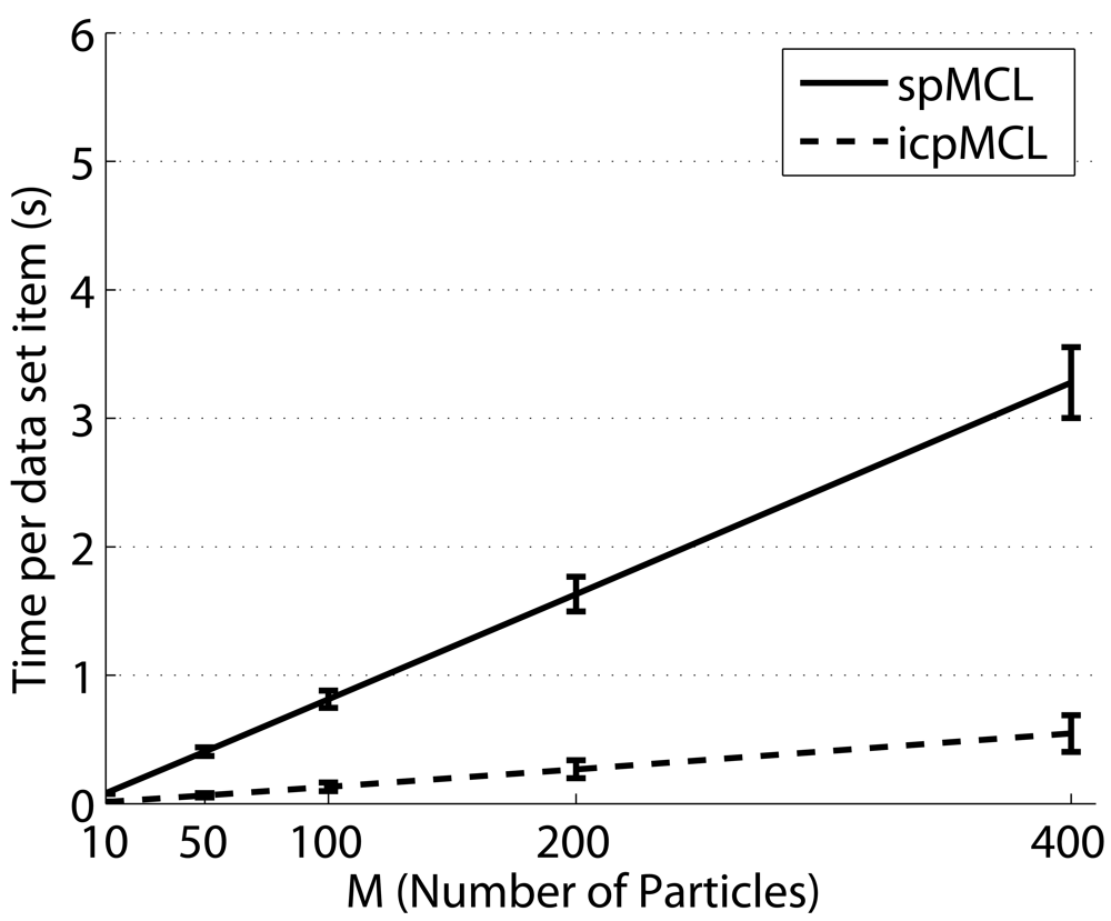
5.2. Evaluating the Influence of the Number of Particles
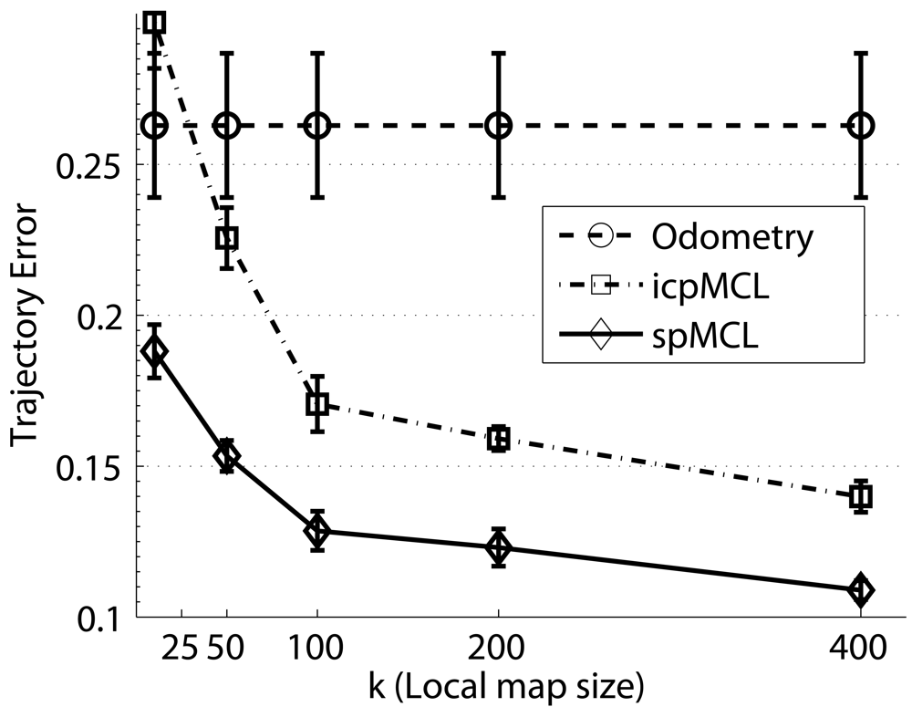
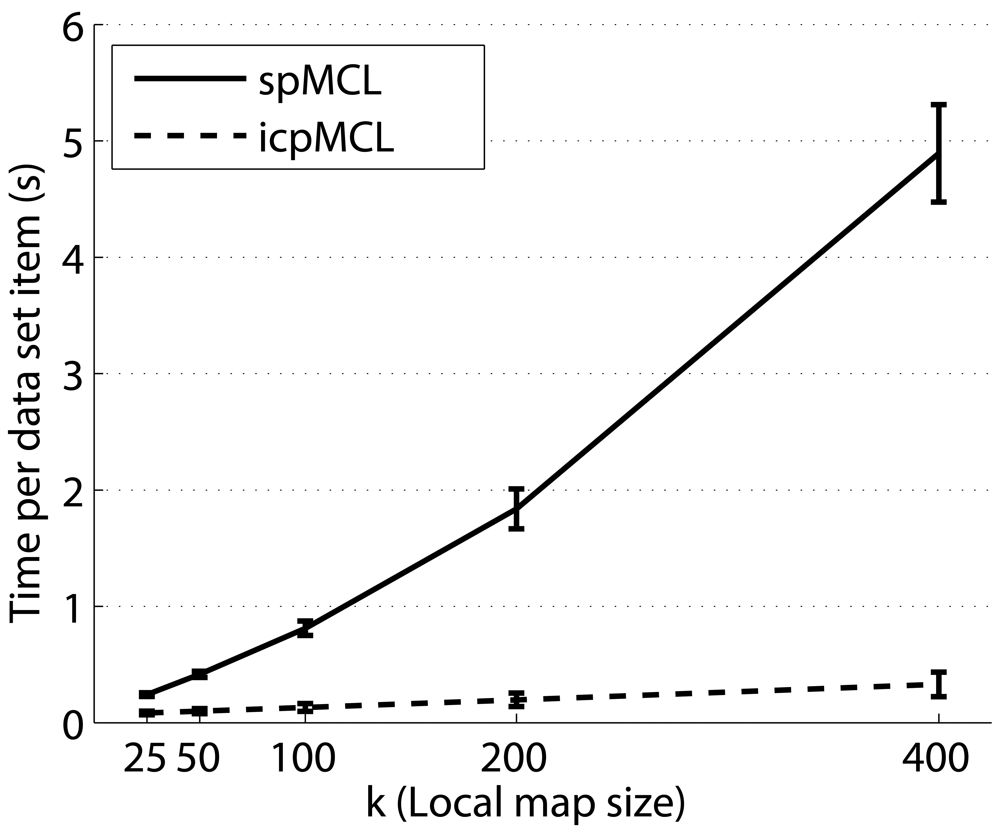
5.3. Evaluating the Influence of the Local Map Size
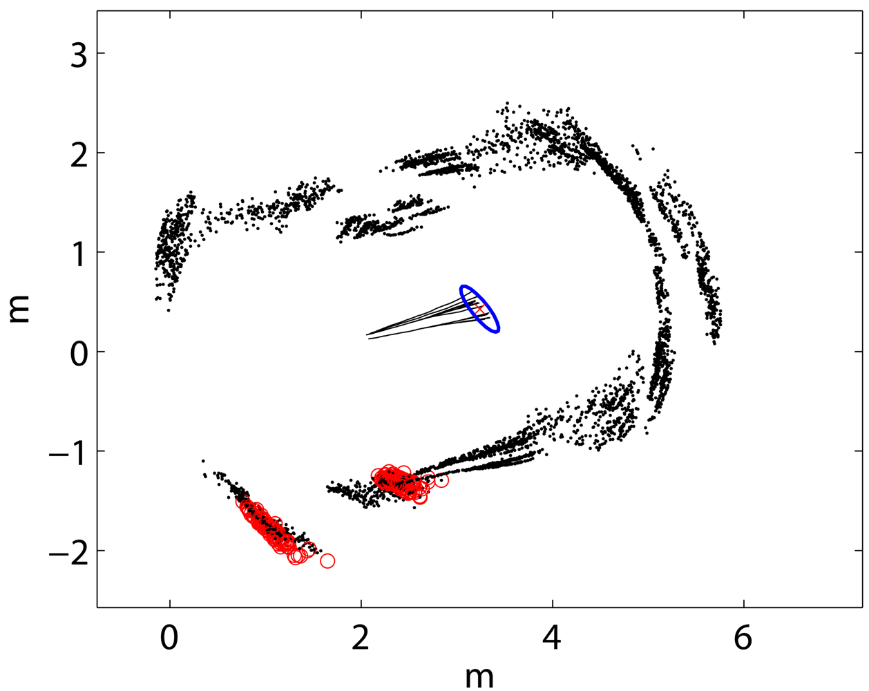
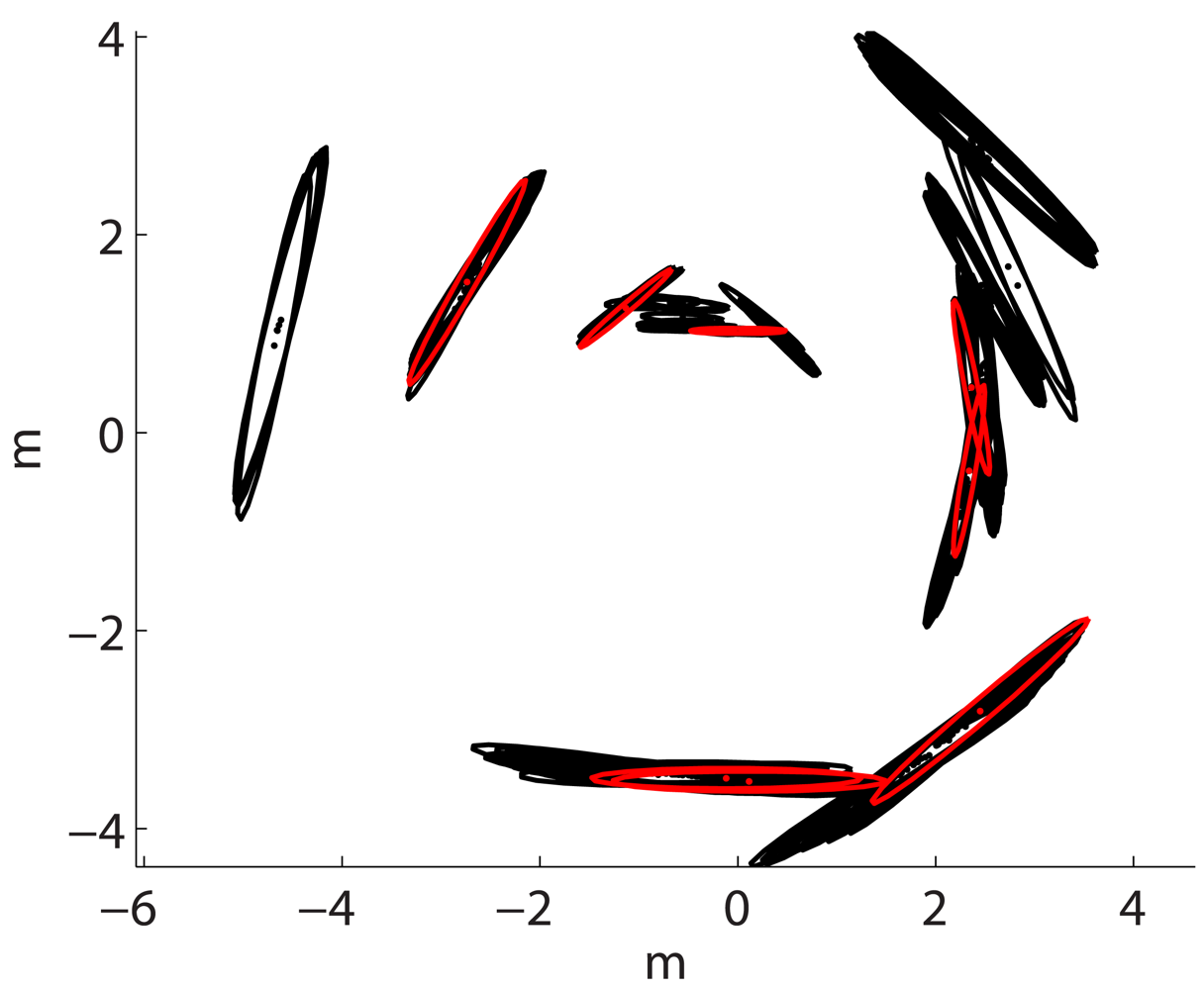
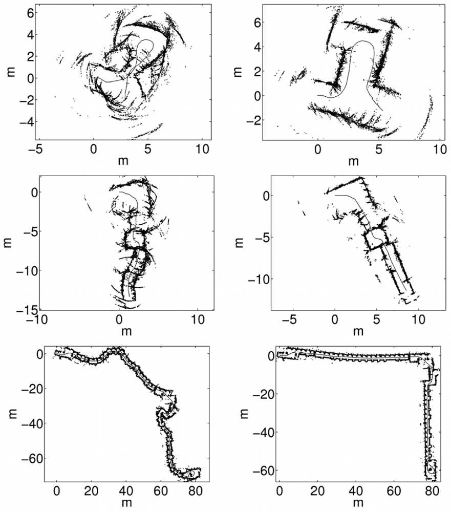
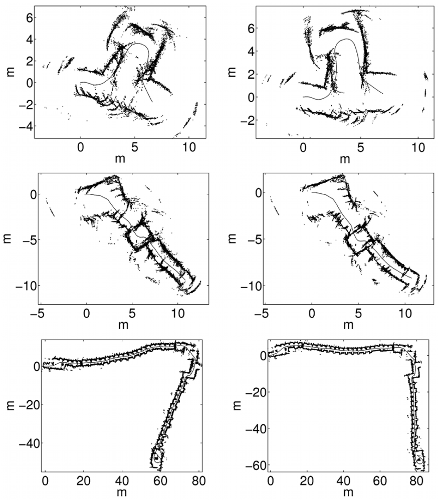
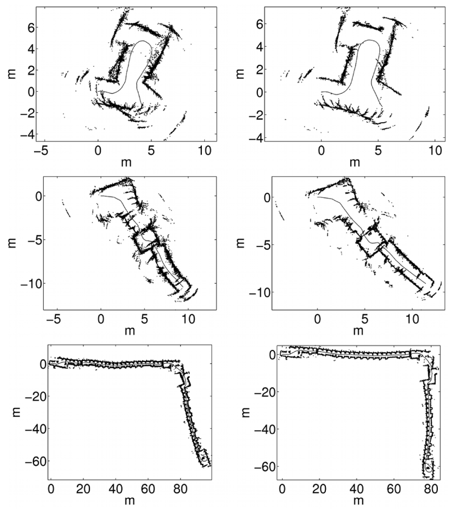
5.4. Qualitative Evaluation
6. Conclusions
Acknowledgments
References
- Tardós, J.D.; Neira, J.; Newman, P.M.; Leonard, J.J. Robust Mapping and Localization in Indoor Environments using Sonar Data. Int. J. Robotics Res. 2002, 21, 311–330. [Google Scholar]
- Groβmann, A.; Poli, R. Robust Mobile Robot Localisation from Sparse and Noisy Proximity Readings Using Hough Transform and Probability Grids. Robot. Auton. Syst. 2001, 37, 1–18. [Google Scholar]
- Burguera, A.; González, Y.; Oliver, G. A Probabilistic Framework for Sonar Scan Matching Localization. Adv. Robot. 2008, 22, 1223–1241. [Google Scholar]
- Hernández, E.; Ridao, P.; Ribas, D.; Batlle, J. MSISpIC: A Probabilistic Scan Matching Algorithm Using a Mechanical Scanned Imaging Sonar. J. Phys. Agents 2009, 3, 3–11. [Google Scholar]
- Choi, Y.H.; Oh, S.Y. Map Building through Pseudo Dense Scan Matching Using Visual Sonar Data. Auton. Robots 2007, 23, 293–304. [Google Scholar]
- Dellaert, F.; Burgard, W.; Thrun, S. Monte Carlo Localization for Mobile Robots. Proceedings of the IEEE International Conference on Robotics and Automation (ICRA), Detroit, MI, USA, May 10–15, 1999.
- Montemerlo, M.; Thrun, S.; Koller, D.; Wegbreit, B. FastSLAM: A Factored Solution to the Simultaneous Localization and Mapping Problem. Proceedings of the AAAI National Conference on Artificial Intelligence, Edmonton, Alberta, Canada, July 28–August 1, 2002.
- Hähnel, D.; Burgard, W.; Fox, D.; Thrun, S. An Efficient FastSLAM Algorithm for Generating Maps of Large-Scale Cyclic Environments from Raw Laser Range Measurements. Proceedings of the IEEE/RSJ International Conference on Intelligent Robots and Systems (IROS), Las Vegas, NV, USA, October 27–31, 2003; 2003. Volume 1. pp. 206–211. [Google Scholar]
- Fox, D.; Burgard, W.; Kruppa, H.; Thrun, S. A Probabilistic Approach to Collaborative Multi-Robot Localization. Autono. Robots 2000, 8, 325–344. [Google Scholar]
- Yaqub, T.; Katupitiya, J. Laser Scan Matching for Measurement Update in a Particle Filter. Proceedings of IEEE/ASME International Conference on Advanced Intelligent Mechatronics, ETH Zurich, Switzerland, September 4–7, 2007; pp. 1–6.
- Thrun, S.; Fox, D.; Burgard, W.; Dellaert, F. Robust Monte Carlo Localization for Mobile Robots. Artif. Intell. 2001, 128, 99–141. [Google Scholar]
- Silver, D.; Morales, D.; Rekleitis, I.; Lisien, B.; Choset, H. Arc Carving: Obtaining Accurate, Low Latency Maps from Ultrasonic Range Sensors. Proceedings of IEEE International Conference on Robotics and Automation, New Orleans, LA, USA, April 26–May 1, 2004; 2, pp. 1554–1561.
- Lu, F.; Milios, E. Robot Pose Estimation in Unknown Environments by Matching 2D Range Scans. J. Intell. Robotic Syst. 1997, 18, 249–275. [Google Scholar]
- Burguera, A.; González, Y.; Oliver, G. Mobile Robot Localization Using Particle Filters and Sonar Sensors. In Advances in Sonar Technology; In-Tech: Vienna, Austria, 2009; Chapter 10; pp. 213–232. [Google Scholar]
- Robotics, A. Pioneer 3™ and Pioneer 2™ H8-Series Operations Manual; ActivMedia Robotics: New York, NY, USA, 2003. [Google Scholar]
- Kleeman, L.; Kuc, R. Sonar Sensing. In Springer Handbook of Robotics; Springer Berlin Heidelberg: Berlin, Germany, 2008; pp. 491–519. [Google Scholar]
- SensComp. 600 Series Instrument Transducer. 2004. Available online: http://www.senscomp.com (accessed on 16 December 2009).
- Moravec, H. Sensor Fusion in Certainty Grids for Mobile Robots. AI Magazine 1988, 9, 61–74. [Google Scholar]
- Blum, F. A Focused, Two Dimensional, Air-Coupled Ultrasonic Array for Non-Contact Generation. Master's Thesis, Georgia Institute of Technology, Atlanta, GA, USA, 2003. [Google Scholar]
- Fonseca, J.; Martins, J.; Couto, C. An Experimental Model For Sonar Sensors. Proceedings of the 1st International Conference on Information Technology in Mechatronics, Istanbul, Turkey, October 1–3, 2001.
- Harris, K.; Recce, M. Experimental Modelling of Time-of-Flight Sonar. Robot. Auton. Syst. 1998, 24, 33–42. [Google Scholar]
- Lee, D. The Map-Building and Exploration Strategies of a Simple Sonar-Equipped Mobile Robot; Cambridge University Press: Cambridge, UK, 1996. [Google Scholar]
- Andreu Mestre, J. Tuning of Odometry and Sonar in a Mobile Robot for Autonomous Navigation Improvement; Graduation project, Departament de Matemàtiques i Informàtica, Universitat de les Illes Balears: Palma, Spain, 2005. (in catalan) [Google Scholar]
- Fox, D.; Burgard, W.; Dellaert, F.; Thrun, S. Monte Carlo Localization: Efficient Position Estimation for Mobile Robots. Proceedings of the 16th National Conference on Artificial Intelligence, Orlando, FL, USA, May 1–5, 1999.
- Smith, R.; Self, M.; Cheeseman, P. Estimating Uncertain Spatial Relationships in Robotics. Proceedings of 1987 IEEE International Conference on Robotics and Automation, Washington, DC, USA, March 1987.
- Thrun, S.; Burgard, W.; Fox, D. Probabilistic Robotics; The MIT Press: Cambridge, MA, USA, 2005. [Google Scholar]
- Montemerlo, M.; Thrun, S.; Koller, D.; Wegbreit, B. FastSLAM 2.0: An Improved Particle Filtering Algorithm for Simultaneous Localization and Mapping that Provably Converges. Proceedings of the Sixteenth International Joint Conference on Artificial Intelligence, Stockholm, Sweden, July 31–August 6, 2003.
- Gustafsson, F.; Gunnarsson, F.; Bergman, N.; Forssell, U.; Jansson, J.; Karlsson, R.; Nordlund, P.J. Particle Filters for Positioning, Navigation and Tracking. IEEE Trans. Signal Process. 2002, 20, 425–437. [Google Scholar]
- Rusinkiewicz, S.; Levoy, M. Efficient Variants of the ICP Algorithm. Proceedings of the 3rd International Conference on 3D Digital Imaging and Modeling (3DIM), Quebec, Canada, May 28–June 1, 2001.
- Biber, P.; Fleck, S.; Strasser, W. A Probabilistic Framework for Robust and Accurate Matching of Point Clouds. Proceedings of the 26th Pattern Recognition Symposium (DAGM), Tubingen, Germany, August 30–September 1, 2004.


© 2009 by the authors; licensee Molecular Diversity Preservation International, Basel, Switzerland. This article is an open access article distributed under the terms and conditions of the Creative Commons Attribution license (http://creativecommons.org/licenses/by/3.0/).
Share and Cite
Burguera, A.; González, Y.; Oliver, G. Sonar Sensor Models and Their Application to Mobile Robot Localization. Sensors 2009, 9, 10217-10243. https://doi.org/10.3390/s91210217
Burguera A, González Y, Oliver G. Sonar Sensor Models and Their Application to Mobile Robot Localization. Sensors. 2009; 9(12):10217-10243. https://doi.org/10.3390/s91210217
Chicago/Turabian StyleBurguera, Antoni, Yolanda González, and Gabriel Oliver. 2009. "Sonar Sensor Models and Their Application to Mobile Robot Localization" Sensors 9, no. 12: 10217-10243. https://doi.org/10.3390/s91210217