1. Introduction
Distance and location measurement systems have many important applications. Local positioning or localization can be achieved through two or more distance measurements. A mobile device, with local positioning techniques, can either gather the information about its position or can be localized from elsewhere. In this context, local-positioning systems attract significant attention [
1].
The chosen technology depends on different circumstances such as outdoor or indoor use, range of distance to be measured, system costs, accuracy,
etc. In most outdoor situations, where a clear line of sight to satellites is available, GPS is the chosen technology. Other available technologies under active research (some for indoor applications) are: sonar [
2,
3], time of flight [
4], radio beacons [
5], systems based on laser-optic technology [
6,
7], vision systems [
8,
9].
Table 1 shows a comparison of different measurement systems.
The prototype described in this paper is a low cost distance measurement system based on pulse repetition between a pair of transceivers. Under these conditions a frequency is generated by the endless travel of the pulse, this frequency is inversely proportional to the time of flight, so the distance between a pair of transceivers can be obtained. The main advantage of our system is that with microsecond electronics it is possible to measure distance with centimeter resolution. A traditional time of flight RF system needs picosecond electronic resolution to get similar distance resolution.
Other advantages of our system over other available and equivalent systems are that our system doesn't need direct vision from transmitters to receivers, as opposed to sonar or laser systems. Our system can be installed indoors, and our design is very cheap (
Table 1).
2. System Description
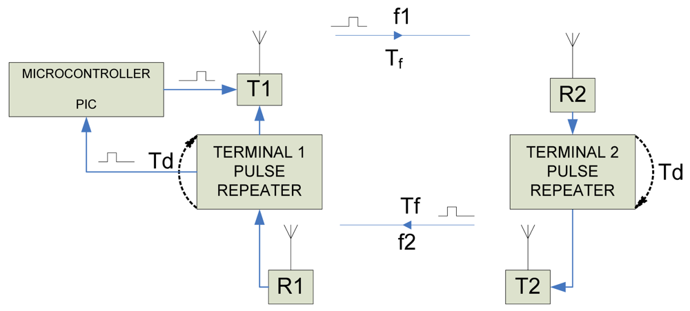
As already mentioned, the proposed measurement system is based on the endless and continuous repetition of an electric pulse that propagates along the distance to be measured (
Figure 1). At both ends of the distance or cable to be measured, there is pulse repetition hardware based on a monostable integrated circuit that generates a new pulse, after a constant delay,
Td, every time a pulse is received, in reality
Td will include all subsystem delays that are the delays introduced also by the transmitter and receiver. Supposing a zero distance is to be measured, the period
T of every cycle will be.
T = 2
Td, because pulse repetitions introduce the same delay at both ends,
Td. If the distance traveled by the wave is considered the new period will be,
T = 2
Td + 2
Tf, where
Tf is the time of flight, which is the time needed for the pulse to travel from terminal 1 to terminal 2 or vice versa, with
T being the time a pulse needs to make a complete circle from terminal 1 to terminal 2 and back, see
Figure1. If
d is the distance to be measured and
v the pulse wave propagation velocity,
, and
being
T the total time to make the circle: which, when expressed as frequency,
f, implies:
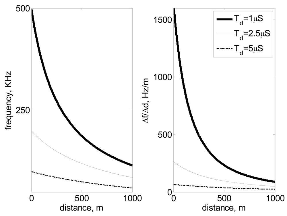
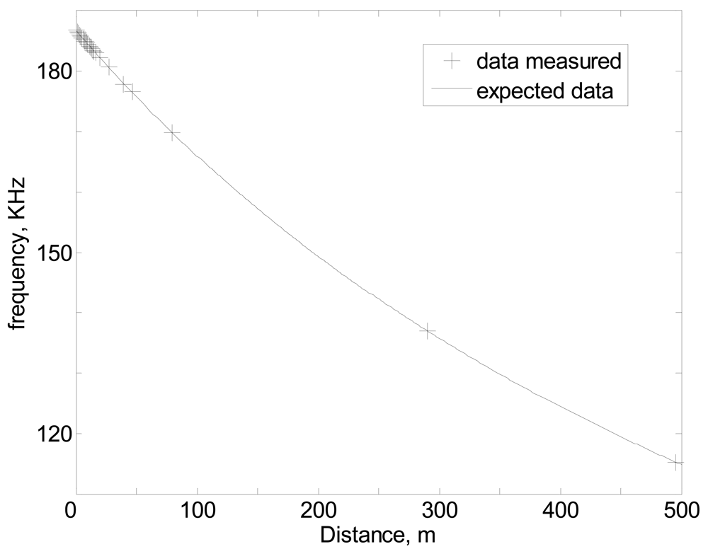
Equation (1) shows that the measured frequency
f decreases as distance
d increases.
The selection of the appropriate repetition delay on both terminals,
Td, will fix the maximum and minimum frequencies captured for a range of distances. The sensitivity diminishes significantly as distance
d increases, as can be seen in
Equation (2) and
Table 1:
Equation (2) shows how the sensitivity
varies significantly with distance d and pulse repetition delay,
Td. One can observe that sensitivity significantly diminishes with both magnitudes.
Figure 2 and
Table 1, show how
f and Δ
f decrease nonlinearly with the distance
d to be measured, following
Equation (1) and
Equation (2) respectively. The selection of an appropriate
Td will depend on the range of distances to be measured and the precision, sensitivity and resolution required. Precision, sensitivity and resolution increase by reducing
Td, but this reduction of
Td has the drawback of increasing the bandwidth and the complexity of the electronic circuit.
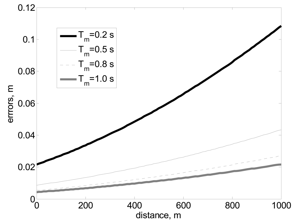
The distance resolution depends also on measurement time. Distance calculation is defined by the frequency measurement, so the precision in the calculation of the frequency of the travelled pulsed is related to the distance resolution.
Figure 3 shows the evolution of errors as a function of the measurement time. When the measurement time is high, the frequency is accurate and the error is low, if the measurement time is low, the error increases.
In our project, the main goal was to locate an autonomous vehicle over a 1 Km
2 area with an accuracy of around 10 cm. In order to achieve this goal,
Td = 2.68
μS is used on the prototype, this implies
and a sensitivity, Δ
f/Δ
d, ranging from 232 to 46 Hz (see
Table 2). The measurement time was fixed at 1 second (
Tm = 1 s). With these parameters 1Hz resolution is obtained for the measured frequency with a theoretical accuracy in
d between 1mm and 4 mm. The real accuracy will be lower due to variances in system parameters and RF bounces. As already mentioned,
Td includes monostable repetition delays, and all other delays. The maximum distance to be measured was 1 Km, and the transmitters have a bigger range.
Real measured data can be observed in
Figure 4, note that real data follows, with a high degree of accuracy, the predicted behavior shown in
Equation (1).
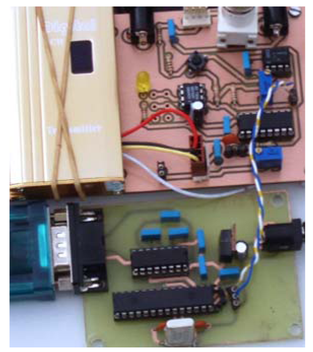
3. Prototype Description
Our prototype as depicted in
Figure 1 is composed of two different terminals, placed at both ends of the distance to be measured. Each terminal is composed of three different elements: 1. Radio frequency pulse transmitter (T1 and T2 in
Figure 1), 2. Monostable Integrated Circuit, needed to repeat and delay the pulse (Pulse Repeater), and 3. Radio frequency pulse receiver, (R1 and R2). Apart from these elements Terminal 1 includes a simple microcontroller (
Figure 5), whose tasks are:
Our system uses two different frequencies to avoid interferences, one frequency f1 to send pulses from terminal 1 to terminal 2 and a second frequency, f2, for pulses from terminal 2 to terminal 1 (see
Figure 1). It is obvious that the same system can be used to measure cable length, for this purpose each terminal should be located at each end of the cable, no radio module is needed because the electric pulse travels through the cable.
The material cost of our prototype, mainly integrated circuit cost, is less than 5 euros when used for cable length measurement and around 100 € when used for distance measurements, but in this last case, around 90% of this cost is for the radio data modules.
4. Cartesian Position of a Mobile System
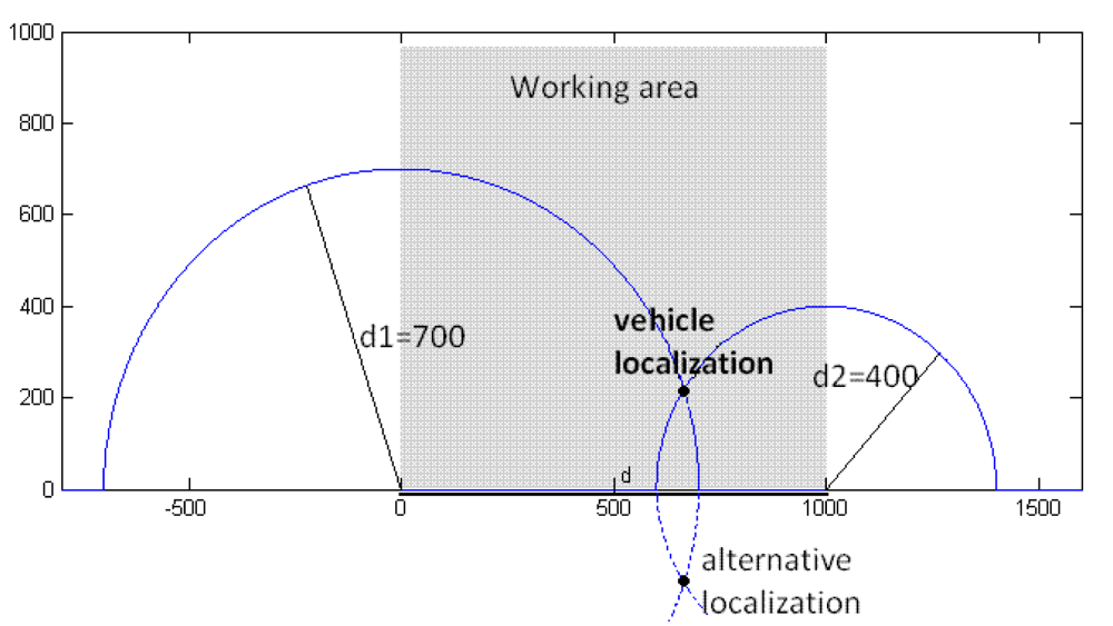
The system described here can be used as a localization system. It's necessary for this application to measure two distances from two different fixed points (see
Figure 6). Calculating the position of the vehicle is determined using these distances. Trilateration is applied in order to resolve the location problem. The localization scheme can be seen in
Figure 6 the distance between the two fixed points (d), and between each one of these fixed points and the vehicle (d1,d2) are known, so the radius of the circumferences can be calculated, see
Figure 6, and the (x,y) Cartesian position is resolved by
equations (3) and
(4).
When this schema with only two measurements (
d1 and
d2) is used, an alternative localization point appears. It's discarded because it is outside the working area. The system only works inside a predefined working area. The radius of each circle is the distance from each fixed point to theproto type. So
Equation (3) is applied in order to calculate the vehicle localization (
x,y):
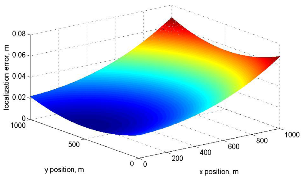
Based on
Equation (4) the system sensitivity,
Equation (5), can be calculated for the Cartesian localization variables (
x,y). The error is presented as a function of the Cartesian positions in
Figure 7. It can be seen a minimum position error at the cartesian position
x = 500,
y = 0. This combination produces a minimum distance (
d1 = 500,
d2 = 500) to each fixed point. According to
Equation (2) and
Figure 3 the minimum error is reached when the distance is small and this is the lowest distance for each distance:
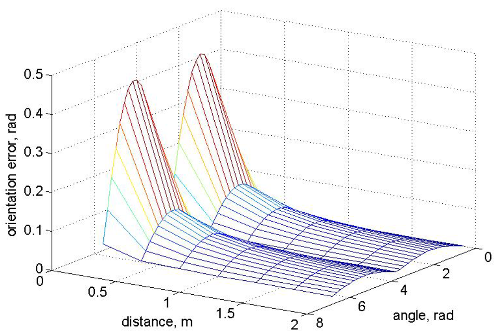
The orientation of the prototype can be obtained if two localization systems are installed on the mobile device. These systems must be separated to get the Cartesian coordinates of each system (
x1,
y1), (
x2,
y2). The prototype orientation can be calculated with these coordinates using
Equation (6) where
xdif is the difference between
x1 and
x2 coordinate and
ydif between
y1 and
y2. The error in the orientation is proportional to the distance of the systems installed in the prototype and the precision in the (
x,y) calculus:
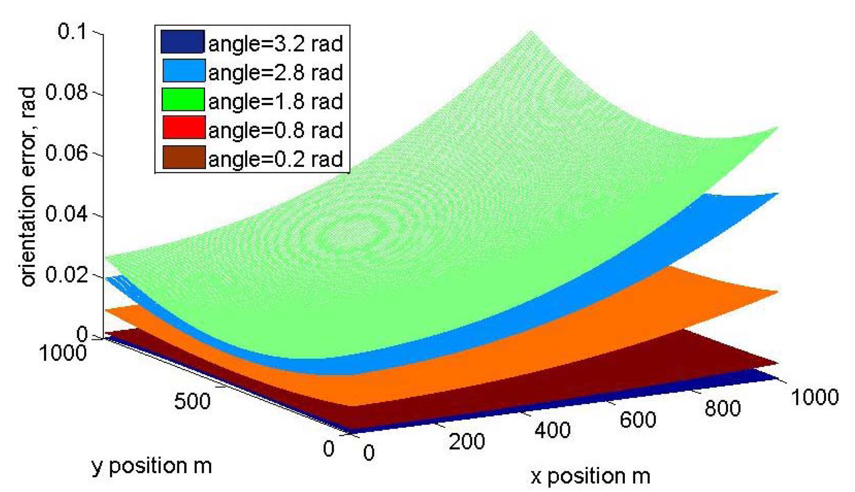
Figure 8 shows the orientation error as a function of the distance between the sensors and orientation angle. The cartesian position of the vehicle is fixed to
x = 500 m,
y = 500 m in this graph. If the error in Cartesian position is represented,
Figure 9 is obtained, where the distance between the two sensors in the prototype is fixed at 1 m. The error as a function of the orientation is plotted with different colors.
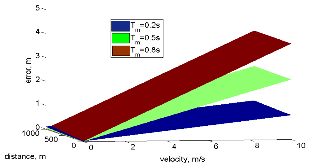
5. Non Static Measurements
If the prototype is moving, the frequency measurement changes as a function of the vehicle velocity
Vν, and measurement time
Tm Equation (7). The error increases with the prototype speed and with the measurement time
Figure 10. For a mobile system better precision is obtained if small measurement times are used. Error will be proportional to
Vν and
Tm so the main error source is proportional to the prototype speed movement.
Figure 10 shows the evolution of error as a function of speed and distance for different measurement times. The main error source is velocity, so in order to get a better distance estimation it's necessary to reduce the measurement time. A detail is presented in
Figure 10 where the nonlinear error as a function of distance can be appreciated:
Another way to see the error is as a measurement delay. Position is not got in real time, the position is obtained
seconds before, when the prototype was located in a previous place. When the system stops, the position will be calculated again with good resolution.


