1. Introduction
Surface soil moisture (
SM) is a variable that plays a crucial role in many processes occurring at the soil-atmosphere interface. The knowledge of the moisture content of the soil over a field or a catchment can be very helpful for hydrological, agronomical and meteorological applications [
1-
2]. Being such an extremely dynamic variable, the possibility of achieving its estimation by means of remote sensing observations is very interesting for many applications [
2]. At present, active microwave (radar) sensors represent the best alternative for a remote
SM estimation for hydrologic and agronomical applications [
1]. The backscattering coefficient (
σ0), obtained from radar sensors, is directly related to the dielectric properties of the soil surface being observed, which is mainly dependent on its moisture content [
3]. Furthermore, the spatial resolution of SAR sensors [
4] and their ability to observe the surface through clouds are aspects that make them interesting for hydrological and agronomical applications.
Radar-based
SM retrieval has been intensively studied in the last decades. Different approaches have been developed and used with varied success [
1]. Among others, the most rigorous approach seems to be the use of electromagnetic scattering models that simulate the surface backscattering process [
3,
5-
11]. Those models can be inverted to retrieve
SM. Several models have been proposed for bare soils or sparsely vegetated surfaces. At present, the Integral Equation Model (IEM) [
5] and the Geometrical Optics Model (GOM) [
3], both physically-based models, are the most frequently used algorithms for soil moisture retrieval [
12-
14]. The former is applicable on smooth or medium roughness conditions and the latter on rough or very rough surfaces. Consequently, both models cover the range of roughness conditions that can be expected over most agricultural surfaces. In addition, these theoretical models have been validated against observations acquired on experimental plots and laboratory settings verifying the adequacy of their predictions as long as their applicability conditions are met [
5,
15,
16].
However, the application of the IEM to natural conditions has been so far problematic [
7,
12,
13,
17-
22]. Frequently, the poor results obtained have been related to the influence of soil roughness on the backscatter [
23]. Furthermore, it has been reported that an accurate field measurement of the required roughness parameters (standard deviation of surface heights
s and correlation length
l), in particular
l, is extremely difficult to perform [
23-
27].
In some circumstances the influence of surface roughness can be simplified. For instance, over agricultural areas where winter cereals are grown, the soil surface remains untilled from sowing (end of October) till harvest (end of June). During this period, surface roughness can be assumed constant and
SM inversion can be simplified assuming that
σ0 variations are only a consequence of
SM dynamics. Of course, over those agricultural areas the vegetation cover can influence the SAR response and complicate the
SM retrieval [
28,
29]. However, in the first stages cereal crops develop slowly and it takes some months until their influence on the SAR signal is significant [
30]. Therefore, during the agricultural inactive period (approximately from November till March for the Spanish watershed studied) the assumption of constant roughness conditions and the use of simplified
SM inversion approaches seems a good choice. In addition, most of the precipitation over temperate climate regions occurs during those autumn and winter months, making the estimation of soil moisture and its dynamics during this period very interesting for hydrological applications.
In autumn and winter periods, severe storms can cause a smoothening of the soil surface, resulting in variations in the surface roughness conditions. The study of the soil surface smoothening caused by precipitation is not new. Many investigations have been carried out on this subject, mostly by soil erosion scientists willing to characterize the detachment and transport of soil particles by rainfall and runoff [
31]. Indeed, surface roughness is an important variable on hydrological and erosion processes and its knowledge is important for many simulation models in these fields. Most of the studies performed to evaluate the soil surface smoothening by precipitation were conducted on laboratory conditions or experimental plots using artificial rainfall simulators. Results evidenced a reduction on the surface roughness as a result of the disintegration and relocation of soil aggregates caused by precipitation. The reduction of the standard deviation of surface heights has been described as an exponential function of the accumulated precipitation or the accumulated kinetic energy of precipitation [
31]. This type of exponential decay functions have been incorporated to widely known erosion models such as the EUROpean Soil Erosion Model EUROSEM [
32].
The above mentioned studies were performed using rainfall simulators that generated very high precipitation rates which are far more intense than observed during normal precipitations of temperate areas [
31]. So, it is interesting to evaluate the variation of roughness under real precipitation conditions. Besides, even if the reduction of the parameter
s has been frequently evidenced, the evolution of the correlation length
l has barely been studied (e.g. [
24]), and little is known on its variations with precipitation. Consequently, it is important to evaluate the variations of surface roughness that can occur over those winter cereal growing areas and to assess their influence on the estimation of soil moisture from radar data.
Roughness parameters are also very variable in space [
31,
33-
35]. Generally, SAR-based
SM estimations are made at the field or catchment scale. Point or pixel estimates are not realistic due to the influence of speckle and roughness spatial variability, therefore aggregation to the field or catchment level is preferable. Nevertheless, catchment and field scale
SM estimates are still very valuable for most applications. Yet, roughness spatial variability can still exert a strong influence on the retrieval of
SM at those scales. The measurement or estimation of field average roughness parameters can be extremely difficult over agricultural and natural surfaces, and the influence of an inaccurate estimation on
s and
l can have consequences on the retrieval of
SM. Yet the quantification of this impact has never been explicitly evaluated to our knowledge.
In this study, we present the results of an intensive campaign of roughness ground measurements and analyze the field scale variability and temporal dynamics of roughness parameters during a winter cereal season. Next, their implications on the estimation of σ0 using the IEM and on the subsequent retrieval of SM from radar data are evaluated by means of a synthetic analysis. In the analysis, different sensor configurations (polarization, frequency and incidence angle) and soil moisture conditions are considered to investigate any possible relation between the conditions of the observations and the sensitivity to roughness variations.
2. Materials and Methods
2.1. Test site
The research was carried out over a small agricultural watershed located in the Spanish region of Navarre called
La Tejería. This watershed is part of the Experimental Agricultural Watershed Network of Navarre, created by the local Government of Navarre in 1993 and aimed at studying the impact of agriculture on the hydrological resources [
36].
The geographical coordinates of the watershed outlet are 42°44′10.6″N and 1°56′57.2″W. The watershed covers approximately 170 ha with homogeneous slopes of about 12%, and an altitude ranging from 496 to 649 m. Its climate is humid submediterranean, with a mean annual temperature of 13°C. The average annual rainfall is about 700 mm, distributed over approximately 105 days.
The most common soils are Tipic Xerochrepts, which are less than 1 m deep. Those soils have Silty-Clay texture (43% clay, 5% sand, 52% silt) and cover most of the hillslopes. The watershed is almost completely cultivated and the hedgerows and streams are the only areas covered by natural vegetation. The main crops are winter cereals (wheat, barley and oat) and less frequently rain fed vegetables (chickpeas and beans) and sunflower. Normally, the growing cycle starts in September when soil preparation and tillage operations are performed. Soil preparation operations consist of a deep tillage operation (usually moldboard plowing); a second operation to break the soil clods and refine the surface using a spike harrow (this harrowing operation is usually applied twice); finally, the cereal is sown (approximately around October) and, in some few fields, the soil surface is compacted afterwards using a roller.
2.2. Ground measurements
Surface roughness measurements were performed during the agricultural year 2004-2005. Ten control fields were selected over the catchment, with field sizes ranging from 3.0 ha to 7.3 ha. Ground measurements were performed on eight dates: 22/09/2004, 08/10/2004, 24/10/2004, 12/11/2004, 28/11/2004, 17/12/2004 and 01/03/2005. Four profiles were acquired per field on each date (with few exceptions, see
Table 1), making a total of 264 profiles. On the first three dates different tillage classes were measured, from the fourth date onward, the cereal crop was sown and the tillage state was classified as ‘Seedbed’ (
Table 1). After March, the vegetation cover is, in general, sufficiently developed to protect the soil surface from the impact of precipitation, so no further measurements were acquired later in the season. In classes where clear tillage rows were observed, profiles were acquired in parallel to the rows, in order to reflect the random component of roughness. Measurements perpendicular to the rows were not performed, since the periodic pattern introduced by the rows should be removed from the obtained roughness profile, and accounted for separately in the backscatter model [
3].
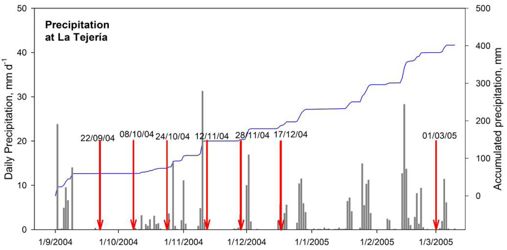
During the research period, the accumulated precipitation was 382 mm, which can be considered normal in the region [
36]. Precipitations were scarce on the first dates and more frequent during winter months (
Figure 1).
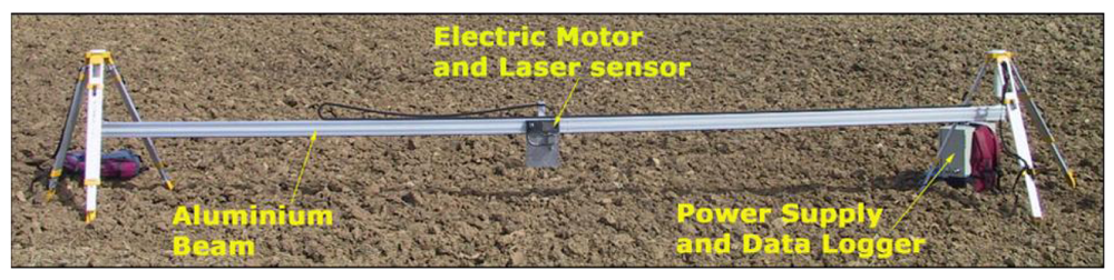
Surface roughness measurements were performed using a non-contact profilometer that incorporates a laser sensor to measure the distance from a reference beam to the soil surface (
Figure 2). The main advantages of the instrument comparing to other roughness measuring methods consist of the facts that the soil surface remains unchanged after the measurement, the profile data are directly downloaded, omitting the need of post-processing, and the very high accuracy of the instrument.
The laser profilometer consists of an aluminium beam, attached to two tripods at both ends (
Figure 2). A laser sensor is placed on a small carriage that is moved along the beam driven by a small electric motor. The laser sensor has a vertical accuracy of 1 mm and is programmed to acquire and store height data every 5 mm. The total length of acquired profiles is 5 m, and the beam can be dismantled in two pieces to be more easily handled and transported. Two plastic racks are attached to the aluminium beam; the former is used by the motor gear to move the carriage and the latter to provide a distance reference to the sensor from which the instrument infers when measurements need to be stored. The instrument is connected to a power supply unit that also contains the data logger.
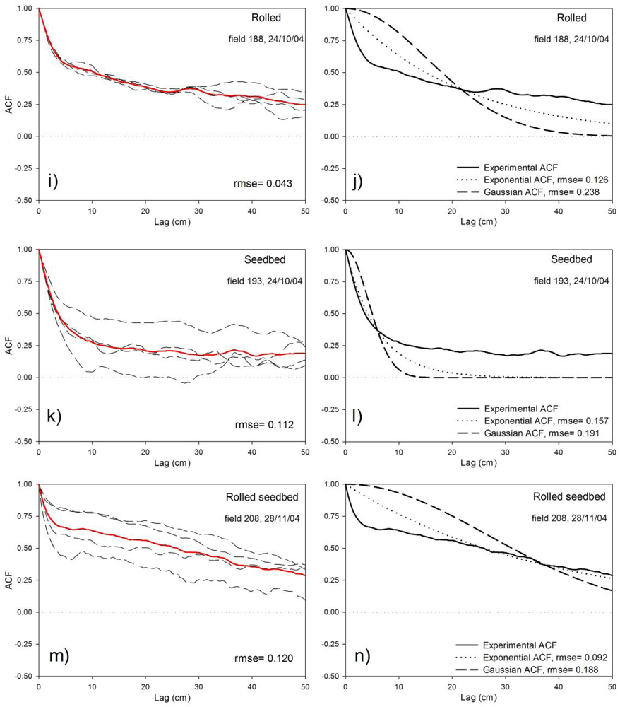
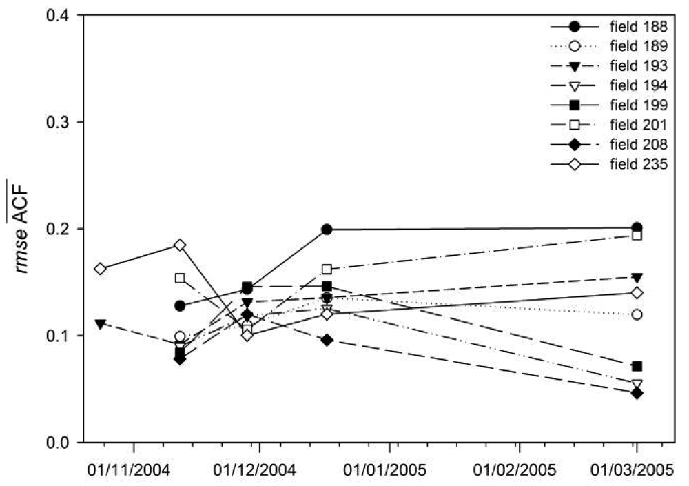
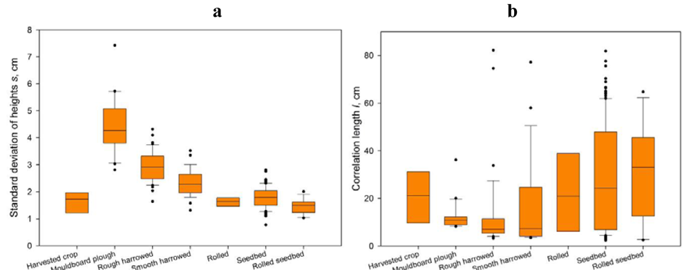
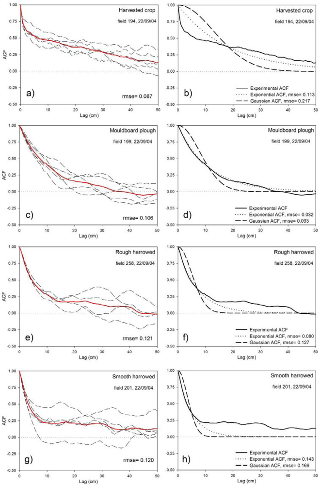
The processing of the profiles acquired is simple and fast. Once profiles are downloaded from the data logger to a PC, the beam deformation is corrected using a parabolic curve fitted to a set of reference measurements acquired in the lab. Afterwards, any shape or trend corresponding to the surface topography is removed. Finally, roughness parameters (s and l) are calculated. Field average s values were obtained as the arithmetic mean of individual s data, whereas average l values were derived from the average autocorrelation function (ACF) calculated using the ACFs of individual profiles.
2.3. Backscatter model
The IEM was used in order to evaluate the influence of roughness variations in the backscattering coefficient of surfaces. In the present research, a simplified version of the IEM was applied which considered only the single scattering term of the backscattered wave [
5,
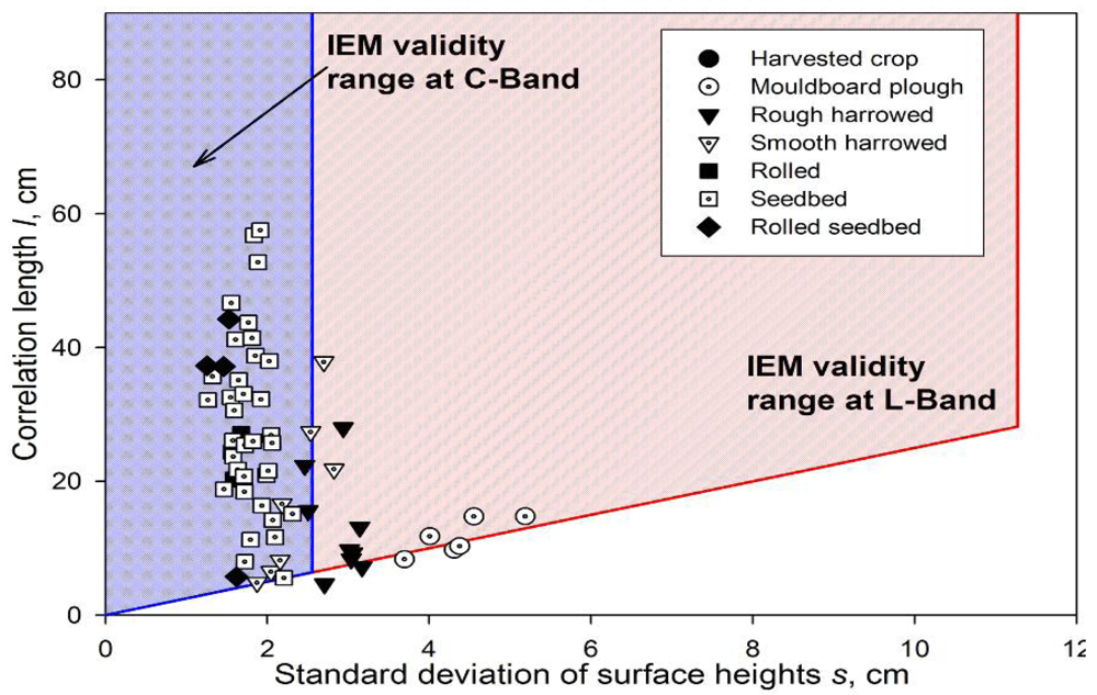
17]. This version is applicable to surfaces with small to moderate roughness conditions or at low to medium frequencies, having a validity range restricted by
ks < 3 and
m < 0.4; with
k being the wave number and
m the surface roughness slope, which for exponentially autocorrelated surfaces equals
s/l. The description of the model can be found in the literature (for instance in [
5,
13,
17]).
It should be remarked that the aim of the study is not to compare the accuracy of IEM estimations with observed SAR data. The intent is to evaluate the importance of roughness variations. Therefore, no actual SAR data were analysed in this study. A basic assumption of the study is that the IEM provides adequate backscatter simulations as long as its applicability conditions are met.
The IEM calculates the backscattering coefficient from a surface given its roughness parameters (
s, l) and exponential
ACF (valid for different soil tillages [
24]), its dielectric constant (
ε) and the scene acquisition parameters: frequency, incidence angle and polarization. In the present research,
εwas calculated through the Dielectric Mixing Model [
37] using
SM, soil texture and temperature data.
After inverting the model, the dielectric constant, and hence SM, can be retrieved from σ0 observations given the roughness parameters. In this paper the inversion was performed using a look-up-table type scheme. In order to prevent the model from predicting physically impossible SM values, the inverted SM values were limited to a range between 0.001 cm3cm-3 and 0.600 cm3cm-3.
2.4. Synthetic analysis
Synthetic analyses based on backscatter models have been used frequently to circumvent the rare availability of extensive SAR observations coincident with high amounts of accurate ground measurements. In the SAR-based soil moisture retrieval literature synthetic studies based on the IEM have been performed with several objectives: (1) to derive or to validate simplified (semi-empirical) models [
6,
7,
9,
10,
38]; (2) to develop statistical retrieval methods based on neural networks [
12,
39-
41]; Bayesian techniques [
28,
42]; or possibilistic algorithms [
43] and fuzzy rule-based models [
44]; (3) to perform sensitivity and error analyses [
10,
13,
17,
20,
23,
45-
48]; and (4) to analyze the influence of roughness measurements' profile length on the calculated backscattering coefficient [
49-
50].
Ideally, synthetic studies should be completed with experimental observations, so the use and interpretation of their results must be cautious. Nonetheless, they are useful to reveal trends or to test different hypothesis, especially in cases where different parameters interact or vary and the interpretation of experimental SAR data becomes difficult.
The synthetic analysis, discussed in this paper, was focused on seedbed fields where the simplifying approaches mentioned in the introduction (constant roughness conditions) could be applied. Several sensor configurations were considered in order to assess their influence on the accuracy of the retrievals. Selected configurations corresponded to those of available spaceborne SAR sensors (i.e. ERS-2, RADARSAT-1/-2, ENVISAT/ASAR and ALOS/PALSAR), thus the results obtained can be linked to different sensors. Regarding polarization, HH and VV configurations were considered since they are more adequate for soil moisture retrieval than cross-polarized configurations [
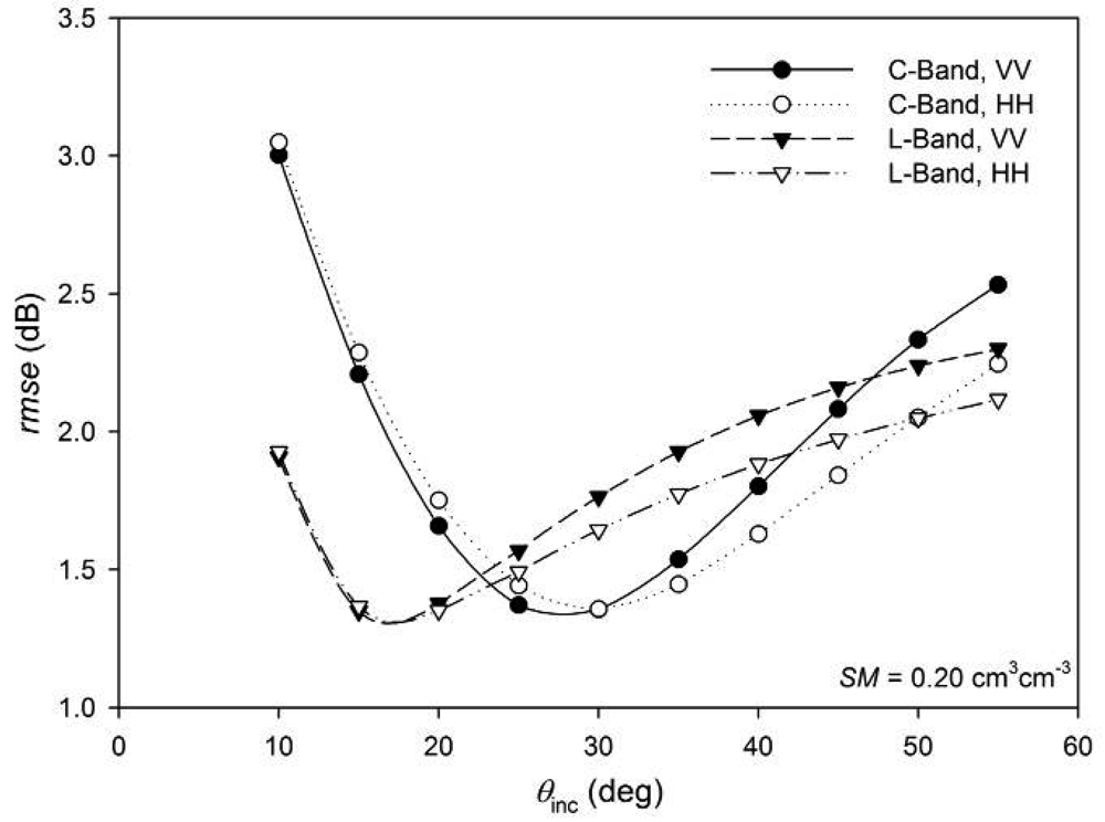
3]. Three incidence angle conditions were used: 15°, 30° and 45°, which correspond to steep, medium and large incidence angles selectable in most sensors. Finally, two frequencies were selected, C-band (5.3 GHz) and L-band (1.27 GHz).
Three different soil moisture conditions were tested: 0.05 cm3cm-3 (dry), 0.20 cm3cm-3 (medium) and 0.35 cm3cm-3 (wet), in an attempt to evaluate whether the influence of roughness was related to the moisture of soils being observed. Finally, the following soil characteristics (necessary to transform SM values to dielectric constant) were considered: sand fraction = 10 %, clay fraction = 35 %, bulk density = 1.4 g cm-3 and soil temperature = 10 °C.
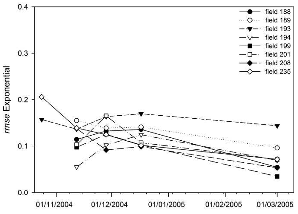
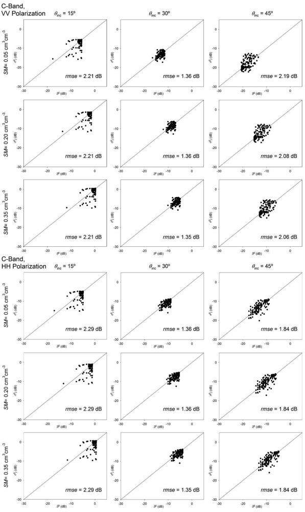
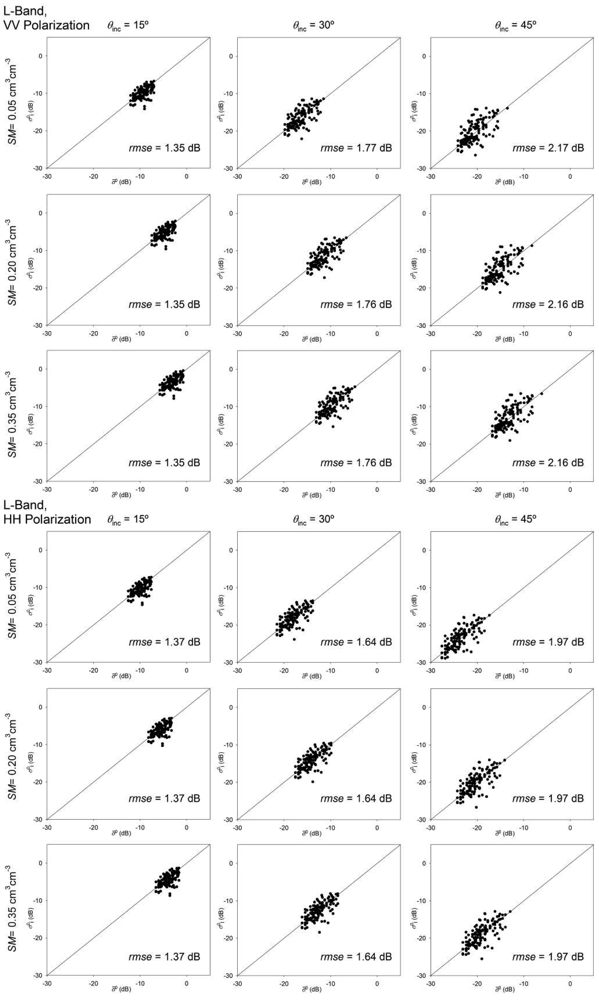
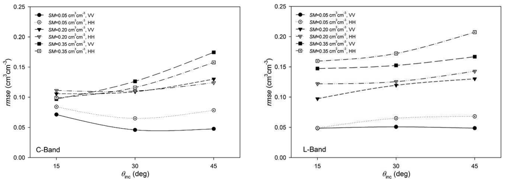
First, IEM simulations were carried out to evaluate the influence of the field scale variability of the roughness parameters on σ0 and on the retrieved SM. Therefore, field average σ0 values were calculated using average roughness parameters which were then compared to the σ0 values calculated from s and l of the individual profiles. The differences were quantified calculating the root mean square error (rmse) in dB. In the inverse simulations, SM was retrieved using field average s and l values and σ0 obtained from individual profile data. The deviations from the initially set SM values (0.05, 0.20 or 0.35) were calculated, those can be an indicator of the influence of field scale roughness variability on the retrieved SM values.
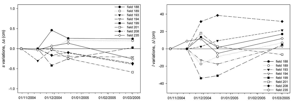
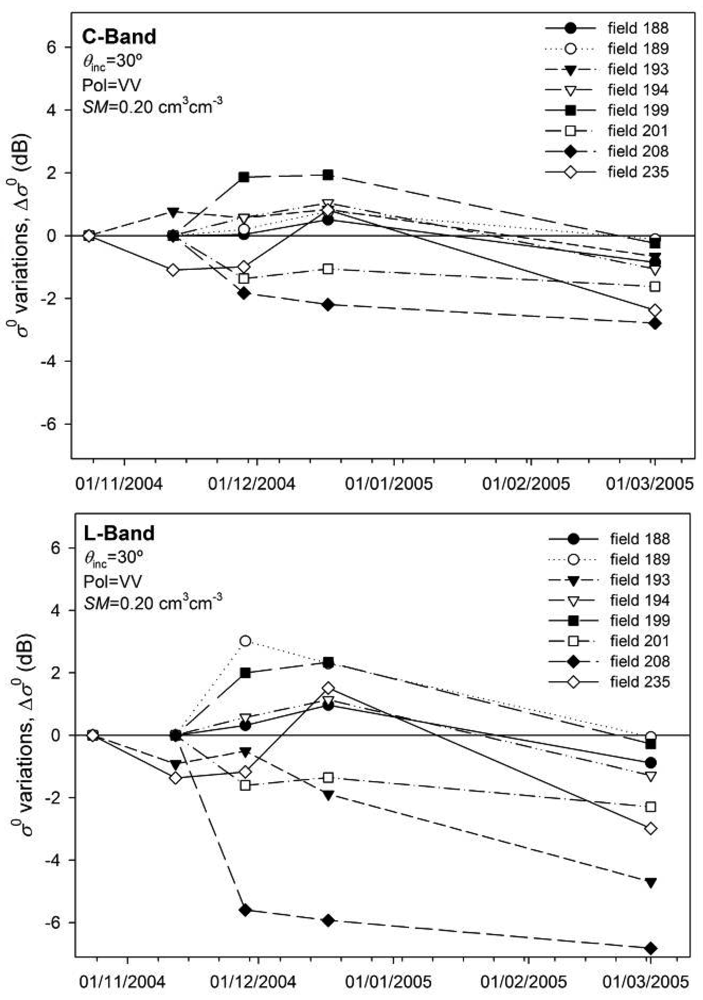
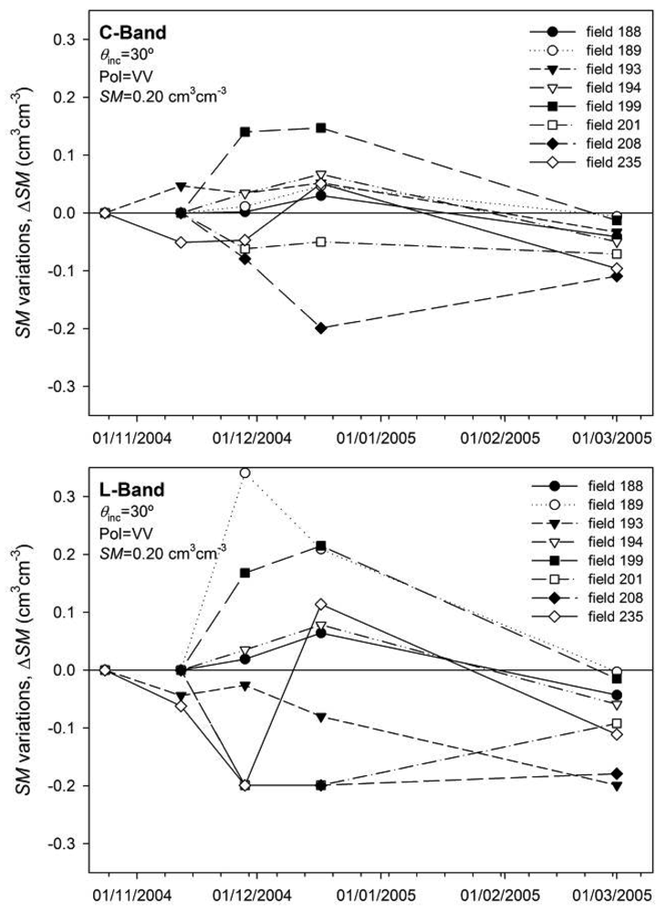
Next, the IEM was used to convert the temporal variations of roughness to variations on the σ0 and on the retrieved SM. In this case, for each field the σ0 calculated for the first seedbed date was compared to those calculated on the subsequent dates. The variations on σ0 calculated this way, were only caused by the temporal variations of roughness since all the other parameters (SM, sensor configuration, etc.) were kept constant. In the inverse mode, SM was retrieved using s and l measurements of the first seedbed date and σ0 values obtained using field average s and l values measured on the subsequent dates. The differences between the retrieved SM values and the ones initially set are a consequence of the temporal variations of roughness.
4. Conclusions
The results of this synthetic study suggest that both field scale roughness spatial variability and precipitation induced temporal variations are aspects that need to be taken into account when inverting backscatter to soil moisture.
In addition, both effects seem to be strongly influenced by the incidence angle and frequency of the observations. The accuracy of the SM retrievals varied also strongly depending on the moisture content of soils, with highest errors observed over wet conditions.
Regarding roughness spatial variability a standard deviation of s and l of respectively 0.30 cm and 19.0 cm was observed. This variability could cause an error in the calculated σ0 of approximately 1-3 dB, depending on the acquisition parameters. Such an error would cause an rmse in the retrieval of SM between 0.05 and 0.20 cm3cm-3, approximately. Lowest errors were observed at intermediate incidence angles of around 25°-30° for C-band and 15°-20° for L-band and dry soil conditions.
Concerning roughness temporal variations, even if the reductions of s and increments of l seem minor, both effects appeared to contribute to a more specular like behaviour of the soil surface, that led to an increase in the σ0 at low incidence angles and a decrease at large angles. As a consequence, significant underestimations of SM (even higher than 0.10 cm3cm-3) could be expected if s and l are considered constant and incidence angles are medium or large. The opposite seems to occur at steep angles where the SM could be overestimated. These results suggest that assuming constant roughness conditions along a growing cycle could cause severe inaccuracies in the retrieved SM values.
In summary, the analysis indicates that both the spatial variability and temporal dynamics of surface roughness could cause severe inaccuracies in the retrieval of soil moisture from SAR observations. So far, a very precise characterisation of roughness needs to be carried out in order to obtain sufficiently accurate moisture estimations from SAR data. The results of this analysis should be completed with experimental observations in future studies.

 ,
, 


