Remote Sensing Data with the Conditional Latin Hypercube Sampling and Geostatistical Approach to Delineate Landscape Changes Induced by Large Chronological Physical Disturbances


Abstract
:1. Introduction
2. Methods and Materials
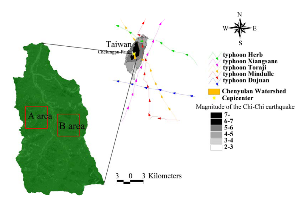
2.1. Study area and remote sensing data
2.2. NDVI
2.3. Variogram and kriging estimation
2.4. Conditional Latin hypercube
- Divide the quantile distribution of X into n strata, and calculate the quantile distribution for each variable, . Calculate the correlation matrix for Z (C).
- Pick n random samples from N; z (i=1,…, n) are the sampled sites. Calculate the correlation matrix of x (T).
- Calculate the objective function. The overall objective function is O = w1O1 + w2O2 + w3O3, , where w is the weight given to each component of the objective function. For general applications, w is set to 1 for all components of the objective function.
- For continuous variables,where is the number of xi that falls between quantiles and
- For categorical data, the objective function is to match the probability distribution for each class of:where η'(xi) is the number of x that belongs to class j in sampled data, and ki is the proportion of class j in X.
- C. To ensure that the correlation of the sampled variables will replicate the original data, another objective function is added:where c is the element of C, the correlation matrix of X, and t is the equivalent element of T, the correlation matrix of x.
- Perform an annealing schedule [50]: M = exp[-ΔO/T], where is the change in the objective function, and T is a cooling temperature (between 0 and 1), which is decreased by a factor d during each iteration.
- Generate a uniform random number between 0 and 1. If rand < M, accept the new values; otherwise, discard changes.
- Try to perform changes: Generate a uniform random number rand. If rand < P, pick a sample randomly from x and swap it with a random site from unsampled sites r. Otherwise, remove the sample(s) from x that has the largest and replace it with a random site(s) from unsampled sites r. End when the value of P is between 0 and 1, indicating that the probability of the search is a random search or systematically replacing the samples that have the worst fit with the strata.
- Go to step 3Repeat steps 3–7 until the objective function value falls beyond a given stop criterion or a specified number of iterations.
2.5. Sequential Gaussian Simulation
- Establish a random path that is visited once and only once, all nodes {ui, i = 1, Λ, N} discretizing the domain of interest Doman. A random visiting sequence ensures that no spatial continuity artifact is introduced into the simulation by a specific path visiting N nodes.
- At the first visited N nodes u1:
- Model, using either a parametric or nonparametric approach, the local ccdf of Z(u1) conditional on n original data {Z (uα), α = 1,Λ, n} FZ (u1; z1|(n)) = prob {Z (u1) ≤ z1|(n)}
- Generate, via the Monte Carlo drawing relation, a simulated value z(l)(u1) from this ccdf FZ (u1: z1|(n)), and add it to the conditioning data set, now of dimension n + 1, to be used for all subsequent local ccdf determinations.
- At the ith node ui along the random path:
- Model the local ccdf of Z(ui) conditional on n original data and the i - 1 near previously simulated values { z(l)(ui), j = 1,Λ, i - 1}:
- Generate a simulated value z(l)(ui) from this ccdf and add it to the conditioning data set, now of dimension n + i.
- Repeat step 3 until all N nodes along the random path are visited.
3. Results and Discussion
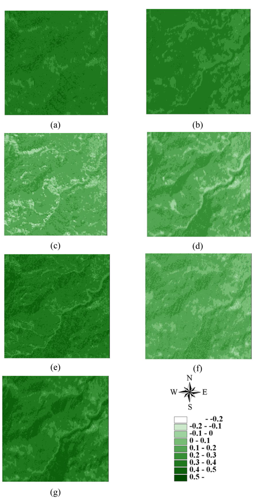
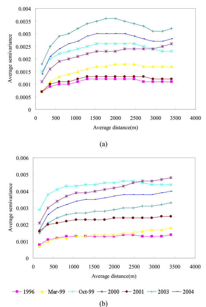
3.1. Statistics and spatial structures of NDVI images
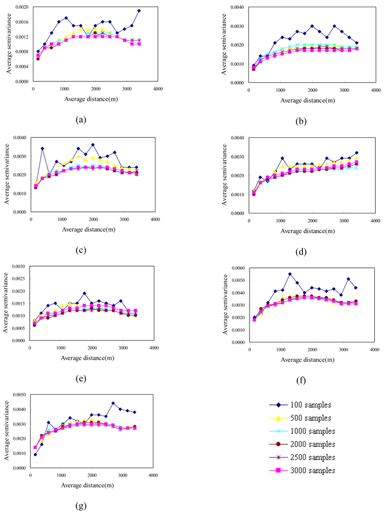
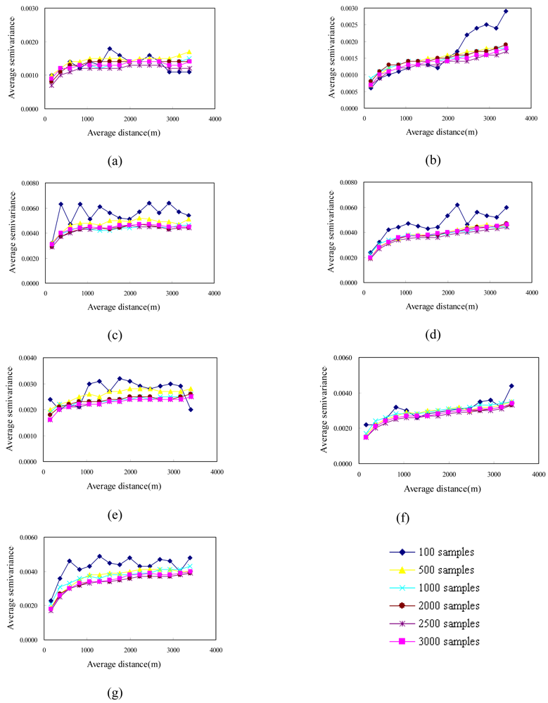
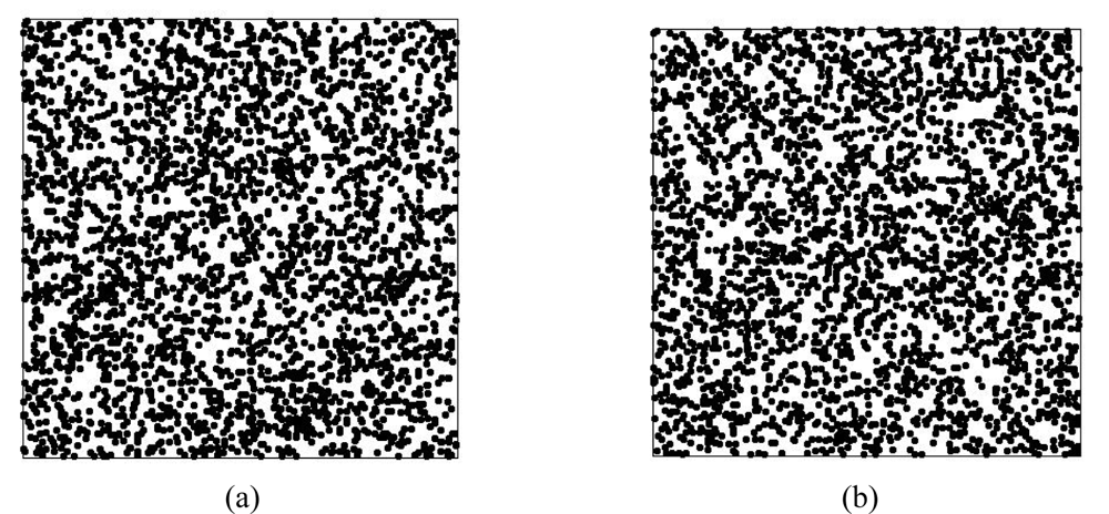
3.2. Latin hypercube sampling for multiple images
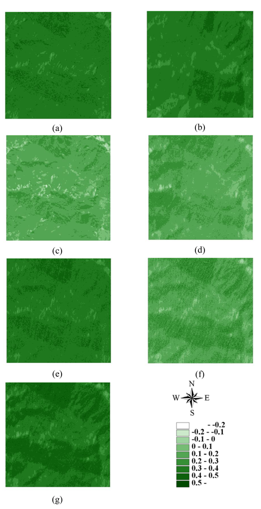
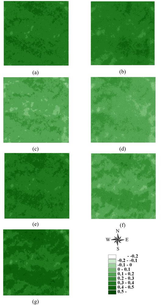
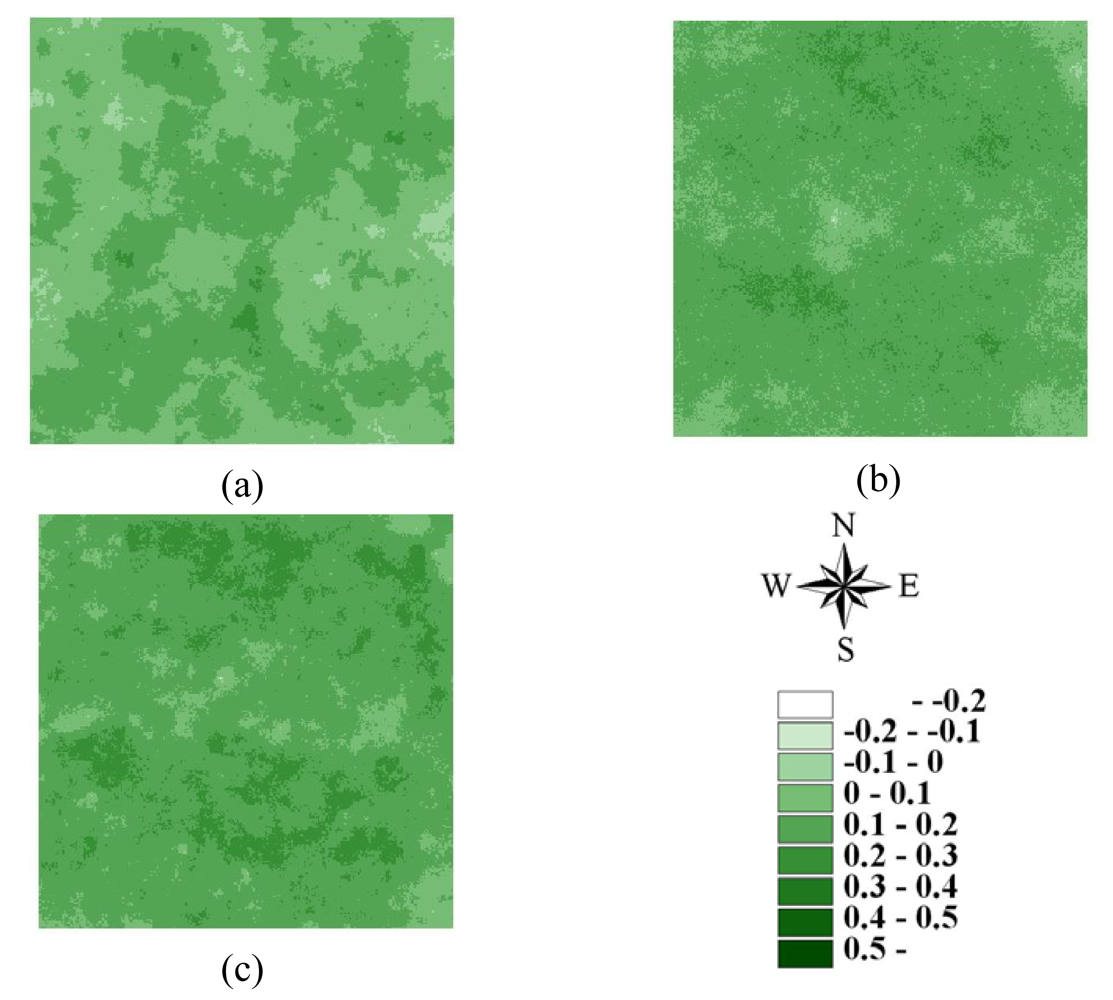
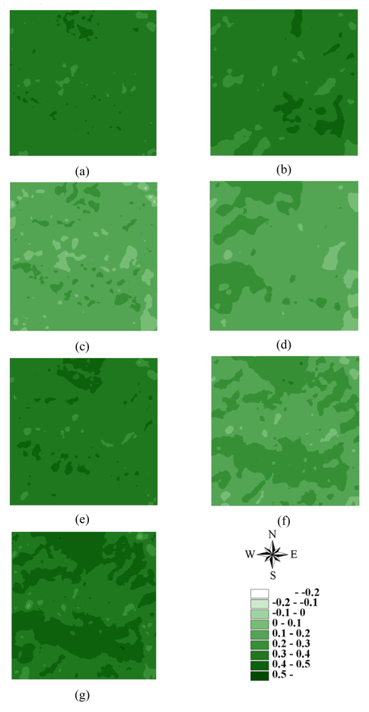
3.3. Estimations and conditional simulations with selected samples
4. Conclusions
Acknowledgments
References
- Foster, D.R.; Knight, D.H.; Franklin, J.F. Landscape patterns and legacies resulting from large, infrequent forest disturbances. Ecosystems 1998, 1, 497–510. [Google Scholar]
- Swanson, F.J.; Johnson, S.L.; Gregory, S.V.; Acker, S.A. Flood disturbance in a forested mountain landscape. Bioscience 1998, 48, 681–689. [Google Scholar]
- Turner, M. G.; Dale, V.H. Comparing large, infrequent disturbances: what have we learned? Ecosystems 1998, 1, 493–496. [Google Scholar]
- Millward, A.A.; Kraft, C.E. Physical influences of landscape on a large-extent ecological disturbance: the northeastern North American ice storm of 1998. Landscape Ecol. 2004, 19, 99–111. [Google Scholar]
- Keefer, D.K. Landslides caused by earthquakes. Geol. Soc. Am. Bul. 1984, 95, 406–421. [Google Scholar]
- Lin, Y.B.; Lin, Y.P; Deng, D.P. Integrating remote sensing data with directional two-dimension wavelet analysis and open geospatial techniques for effective disaster monitoring and management. Sensors 2008, 8, 1070–1089. [Google Scholar]
- Keefer, D.K. The importance of earthquake-induced landslides to long term slope erosion and slope-failure hazards in seismically active regions. Geomorphology 1994, 10, 265–284. [Google Scholar]
- Lee, M.F.; Lin, T.C.; Vadeboncoeur, M.A.; Hwong, J.L. Remote sensing asseeement of forest damage in relation to the 1996 strong typhoon Herb at Lienhuachi Experimental Forest, Taiwan. Forest Ecol. Manag. 2008, 255, 3297–3306. [Google Scholar]
- DeMets, C.; Gordon, R.G.; Argus, D.F.; Stein, S. Current plate motions. Geophys. J. Int. 1990, 104, 425–478. [Google Scholar]
- Lin, C.W.; Liu, S.H.; Lee, S.Y.; Liu, C.C. Impacts of the Chi-Chi earthquake on subsequent rainfall-induced landslides in central Taiwan. Eng. Geol. 2006, 87–101. [Google Scholar]
- Lin, G.W.; Chen, H.; Chen, Y.H.; Horng, M.J. Influence of typhoons and earthquakes on rainfall-induced landslides and suspended sediments discharge. Eng. Geol. 2008, 97, 32–41. [Google Scholar]
- Lin, C.W.; Shieh, C.L.; Yuan, B.D.; Shieh, Y.C.; Liu, S.H.; Lee, S.Y. Impact of Chi-Chi earthquake on the occurrence of landslides and debris flows: example from the Chenyulan River watershed, Nantou, Taiwan. Eng. Geol 2003, 71, 49–61. [Google Scholar]
- Lin, Y.P.; Chang, T.K.; Wu, C.F; Chiang, T.C.; Lin, S.H. Assessing impacts of typhoons and the ChiChi earthquake on Chenyuland watershed landscape patterns in Central Taiwan. Environ. Manage. 2006, 38, 108–125. [Google Scholar]
- Lin, C.Y.; Wu, J.P.; Lin, W.T. The priority of revegetation for the landslides caused by the catastrophic Chi-Chi earthquake at ninety-nine Peaks in Nantoun area. J. Chinese Soil Water Cons. 2001, 32, 59–66. [Google Scholar]
- Sellers, P.J. Modeling the exchange of energy, water, and Carbon between continents and atmosphere. Science 1997, 275, 602–609. [Google Scholar]
- Garrigues, S.; Allard, D.; Baret, F.; Morisette, J. Multivariate quantification of landscape spatial heterogeneity using variogram models. Remote Sens. Environ. 2008, 112, 216–230. [Google Scholar]
- Cohen, W.B.; Goward, S.N. Landsat's role in ecological applications of remote sensing. Bioscience 2004, 54, 535–545. [Google Scholar]
- Hayes, D.J.; Cohen, W.B. Spatial, spectral and temporal patterns of tropical forest cover change as observed with multiple scales of optical satellite data. Remote Sens. Environ. 2007, 106, 1–16. [Google Scholar]
- Tarnavsky, E.; Garrigues, S.; Brown, M.E. Multiscale geostatistical analysis of AVHRR, SPOT-VGT, and MODIS global NDVI products. Remote Sens. Environ. 2008, 112, 535–549. [Google Scholar]
- Lin, W.T.; Chou, W.C.; Lin, C.Y. Earthquake-induced landslide hazard and vegetation recovery assessment using remotely sensed data and a neural network-based classifier: a case study in central Taiwan. Nat. Hazards 2008, 47, 331–347. [Google Scholar]
- Jensen, T.R. Introductory digital image processing: a remote sensing perspective; Prentice Hall: New York, 1996. [Google Scholar]
- Sellers, P.J. Canopy reflectance, photosynthesis and transpiration. Int. J. Remote Sens. 1985, 6, 1335–1372. [Google Scholar]
- Lin, W.T.; Lin, C.Y.; Chou, W.C. Assessment of vegetation recovery and soil erosion at landslides caused by a catastrophic earthquake: a case study in Central Taiwan. Ecol. Eng. 2006, 28, 79–89. [Google Scholar]
- Wiens, J.A. Spatial scaling in ecology. Funct. Ecol. 1989, 3, 385–397. [Google Scholar]
- Urban, D.L.; O'Niell, R.V.; Shugart, H.H. Landscape ecology. Bioscience 1987, 37, 119–127. [Google Scholar]
- Lobo, A.; Moloney, K.; Chic, O.; Chiariello, N. Analysis of fine-scale spatial pattern of a grassland from remotely-sensed imagery and field collected data. Landscape Ecol. 1998, 13, 111–131. [Google Scholar]
- Curran, P.J.; Atkinson, P.M. Geostatistics and remote sensing. Prog. Phys. Geog. 1998, 22, 61–78. [Google Scholar]
- Garrigues, S.; Allard, D.; Baret, F. Modeling temporal changes in surface spatial heterogeneity over an agricultural site. Remote Sens. Environ. 2008, 112, 58–602. [Google Scholar]
- Garrigues, S.; Allard, D.; Baret, F. Influence of the spatial heterogeneity on the non linear estimation of Leaf Area Index from moderate resolution remote sensing data. Remote Sens. Environ. 2006, 106, 286–298. [Google Scholar]
- Fortin, M.J.; Edwards, G. A cognitive view of spatial uncertainty; Hunsaker, C.T., Goodchild, M.F., Friedl, M.A., Case, T.J., Eds.; Springer: New York, 2001; pp. 133–157. [Google Scholar]
- Minasny, B.; McBratney, A.B. The variance quadtree algorithm: use for spatial sampling design. Comput. Geosci. 2007, 33, 383–392. [Google Scholar]
- Edwards, G.; Fortin, M.J. Delineation and analysis of vegetation boundaries, Spatial uncertainty in ecology: implications for remote sensing and GIS application; Hunsaker, C. T., Goodchild, M. A., Friedl, A., Case, T.J., Eds.; Springer: New York, 2001; pp. 158–174. [Google Scholar]
- Thompson, S.K. Sampling; Wiley Interscience: New York, 1992. [Google Scholar]
- Minasny, B.; McBratney, A.B. A conditioned Latin hypercube method for sampling in the presence of ancillary information. Comput. Geosci. 2006, 32, 1378–1388. [Google Scholar]
- McKay, M.D.; Beckman, R.J.; Conover, W.J. A comparison of three methods for selecting values of input variables in the analysis of output from a computer code. Technometrics 1979, 21, 239–245. [Google Scholar]
- Iman, R.L.; Conover, W.J. Small sample sensitivity analysis techniques for computer models, with an application to risk assessment. Commun. Statist. Theory Meth. 1980, A9, 1749–1874. [Google Scholar]
- Lin, Y.P.; Yen, M.H.; Deng, D.P.; Wang, Y.C. Geostatistical Approaches and Optimal Additional Sampling Schemes for Spatial Patterns and Future Samplings of Bird Diversity. Global Ecol. Biogeogr. 2008, 17, 175–188. [Google Scholar]
- Goovaters, P. Geostatistics for Natural Resources Evaluation; Oxford University Press: New York, 1997. [Google Scholar]
- Kyriakidis, P.C. Geostatistical models of uncertainty for spatial data, Spatial uncertainty in ecology: implications for remote sensing and GIS application; Hunsaker, C. T., Goodchild, M. F., Friedl, M.A., Case, T.J., Eds.; Springer: New York, 2001; pp. 175–213. [Google Scholar]
- Deutsch, C.V.; Journel, A. G. GSLIB. Geostatistical Software Library and User's Guide; Oxford University Press: New York, 1992. [Google Scholar]
- Pebesma, E.J.; Heuvelink, G.B.M. Latin hypercube sampling of Gaussian random fields. Technometrics 1999, 41, 303–312. [Google Scholar]
- Zhang, Y.; Pinder, G.F. Latin-hypercube sample-selection strategies for correlated random hydraulic-conductivity fields. Water Resour. Res. 2004, 39. No. 1226. [Google Scholar]
- Xu, C.; He, H. S.; Hu, Y.; Chang, Y.; Li, X.; Bu, R. Latin hypercube sampling and geostatistical modeling of spatial uncertainty in a spatially explicit forest landscape model simulation. Ecol. Model. 2005, 185, 255–269. [Google Scholar]
- Roger, B.; Yu, T.T. The morphology of thrust faulting in the 21 September 1999, Chi-Chi, Taiwan earthquake. J. Asian Earth Sci. 2000, 18, 351–367. [Google Scholar]
- Central Weather Bureau (CWB). 1999. URL: http://scman.cwb.gov.tw/eqv3/eq_report/special/19990921/921 , isomap. GIF.
- Central Weather Bureau. Report on typhoons in 2000; Ministry of Transportation and Communications: Taiwan, 2000; pp. 130–162. [Google Scholar]
- Central Weather Bureau. Report on typhoons in 2001; Ministry of Transportation and Communications: Taiwan, 2001; pp. 84–111. [Google Scholar]
- Central Weather Bureau (CWB). Typhoon Database. 2008. URL: http://rdc28.cwb.gov.tw/.
- Jensen, T.R. Introductory digital image processing: a remote sensing perspective; Prentice Hall: New York, 1996. [Google Scholar]
- Press, W.H.; Flannery, B.T.; Teukolsky, S.A.; Vetterling, W.T. Numerical Recipes in Fortran: The art of Scientific Computing, 2nd ed.; Cambridge University Press: Cambridge, UK, 1992. [Google Scholar]
- Fredericks, A. K.; Newman, K. B. A comparison of the sequential Gaussian and Markov-Bayes simulation methods for small samples. Math. Geol. 1998, 30, 1011–1032. [Google Scholar]
- Ward, D; Phinn, SR; Murray, AT. Monitoring growth in rapidly urbanizing areas using remotely sensed data. Prof. Geogr. 2000, 52, 371–386. [Google Scholar]
- Akiwumi, F.A.; Butler, D.R. Mining and environmental change in Sierra Leone, West Africa: A remote sensing and hydrogeomorphological study. Environ. Monit. Assess. 2008, 142, 309–318. [Google Scholar]
- Giriraj, A; Irfan-Ullah, M; Murthy, MSR; et al. Modelling spatial and temporal forest cover change patterns (1973-2020): A case study from South Western Ghats (India). Sensors 2008, 8, 6132–6153. [Google Scholar]
- Fox, D.M.; Maselli, F.; Carrega, P. Using SPOT images and field sampling to map burn severity and vegetation factors affecting post forest fire erosion risk. Catena 2008, 75, 326–335. [Google Scholar]
- Zomeni, M.; Tzanopoulos, J.; Pantis, J.D. Historical analysis of landscape change using remote sensing techniques: An explanatory tool for agricultural transformation in Greek rural areas. Landscape Urban Plan. 2008, 86, 38–46. [Google Scholar]
- Chang, K.T.; Chiang, S.H.; Hsu, M.L. Modeling typhoon- and earthquake- induced landslides in a mountains watershed using logistic regression. Geomorphology 2007, 89, 335–347. [Google Scholar]


| Area | Date | Mean | Std. | Min. | Max. |
|---|---|---|---|---|---|
| A | 1996/11/08 | 0.36 | 0.04 | 0.11 | 0.48 |
| 1999/03/06 | 0.32 | 0.04 | 0.13 | 0.43 | |
| 1999/10/31 | 0.14 | 0.07 | -0.22 | 0.33 | |
| 2000/11/27 | 0.15 | 0.07 | -0.14 | 0.35 | |
| 2001/11/20 | 0.37 | 0.05 | 0.03 | 0.50 | |
| 2003/12/17 | 0.15 | 0.06 | -0.12 | 0.33 | |
| 2004/11/19 | 0.35 | 0.06 | 0.05 | 0.54 | |
| B | 1996/11/08 | 0.36 | 0.03 | 0.13 | 0.47 |
| 1999/03/06 | 0.36 | 0.04 | 0.14 | 0.48 | |
| 1999/10/31 | 0.16 | 0.05 | -0.20 | 0.38 | |
| 2000/11/27 | 0.17 | 0.05 | -0.09 | 0.33 | |
| 2001/11/20 | 0.37 | 0.04 | 0.14 | 0.48 | |
| 2003/12/17 | 0.20 | 0.06 | -0.08 | 0.44 | |
| 2004/11/19 | 0.39 | 0.05 | 0.10 | 0.57 | |
| Area | Date | Model | Parameters | The fit | Cross-validate |
|---|---|---|---|---|---|
| A | 1996/11/08 | Exponential model | C0=0.000453, C0+C=0.001212, R=1204.000 | (SS=7.774E-08; r2=0.832, C0/C0+C=0.374) | r2 =0.722 |
| 1999/03/06 | Exponential model | C0=0.000147, C0+C=0.001744; R=1278.000 | (SS=3.490E-08; r2=0.978, C0/C0+C=0.084) | r2=0.893 | |
| 1999/10/31 | Exponential model | C0=0.000878, C0+C=0.002496; R=1020.000 | (SS=1.573E-07; r2=0.873,C0/C0+C=0.352) | r2=0.839 | |
| 2000/11/27 | Exponential model | C0=0.000761, C0+C=0.002452; R=1881.000 | (SS=18.597E-08; r2=0.961, C0/C0+C=0.310) | r2=0.894 | |
| 2001/11/20 | Exponential model | C0=0.000518, C0+C=0.001294; R=1497.000 | (SS=5.124E-08; r2=0.878, C0/C0+C=0.400) | r2=0.723 | |
| 2003/12/17 | Exponential model | C0=0.000700, C0+C=0.003370; R=981.000 | (SS=3.420E-07; r2=0.893, C0/C0+C=0.208) | r2=0.737 | |
| 2004/11/19 | Exponential model | C0=0.000229, C0+C=0.002878; R=918.000 | (SS=1.918E-07; r2=0.930, C0/C0+C=0.080) | r2=0.862 | |
| B | 1996/11/08 | Exponential model | C0=0.000138, C0+C=0.001326; R=654.000 | (SS=1.610E-08; r2=0.953, C0/C0+C=0.104) | r2=0.781 |
| 1999/03/06 | Exponential model | C0=0.000712, C0+C=0.001814; R=4620.000 | (SS=6.070E-08; r2=0.945, C0/C0+C=0.393) | r2=0.901 | |
| 1999/10/31 | Exponential model | C0=0.000590, C0+C=0.004440; R=564.000 | (SS=1.678E-07; r2=0.939, C0/C0+C=0.133) | r2=0.849 | |
| 2000/11/27 | Exponential model | C0=0.0001863, C0+C=0.004676; R=2646.000 | (SS=2.474E-07; r2=0.952, C0/C0+C=0.398) | r2=0.908 | |
| 2001/11/20 | Exponential model | C0=0.0001205, C0+C=0.002429; R=1281.000 | (SS=5.621E-08; r2=0.933, C0/C0+C=0.498) | r2=0.728 | |
| 2003/12/17 | Exponential model | C0=0.0001258, C0+C=0.003126; R=2298.000 | (SS=1.567E-07; r2=0.949, C0/C0+C=0.402) | r2=0.820 | |
| 2004/11/19 | Exponential model | C0=0.0001161, C0+C=0.003832; R=1680.000 | (SS=1.186E-07; r2=0.977, C0/C0+C=0.303) | r2=0.902 |
| Area | Date | Mean | Std. | Min. | Max. | Area | Date | Mean | Std. | Min. | Max. | ||
|---|---|---|---|---|---|---|---|---|---|---|---|---|---|
| 100 | A | 1996/11/08 | 0.36 | 0.04 | 0.22 | 0.44 | 1,000 | A | 1996/11/08 | 0.36 | 0.03 | 0.17 | 0.45 |
| 1999/03/06 | 0.36 | 0.05 | 0.22 | 0.45 | 1999/03/06 | 0.36 | 0.04 | 0.17 | 0.47 | ||||
| 1999/10/31 | 0.16 | 0.05 | 0.00 | 0.24 | 1999/10/31 | 0.16 | 0.05 | -0.10 | 0.33 | ||||
| 2000/11/27 | 0.17 | 0.05 | 0.00 | 0.28 | 2000/11/27 | 0.17 | 0.05 | 0.00 | 0.33 | ||||
| 2001/11/20 | 0.37 | 0.04 | 0.19 | 0.44 | 2001/11/20 | 0.37 | 0.04 | 0.20 | 0.46 | ||||
| 2003/12/17 | 0.19 | 0.06 | 0.01 | 0.33 | 2003/12/17 | 0.20 | 0.06 | 0.00 | 0.38 | ||||
| 2004/11/19 | 0.39 | 0.05 | 0.19 | 0.05 | 2004/11/19 | 0.40 | 0.05 | 0.17 | 0.54 | ||||
| B | 1996/11/08 | 0.36 | 0.04 | 0.24 | 0.44 | B | 1996/11/08 | 0.16 | 0.07 | 0.00 | 0.30 | ||
| 1999/03/06 | 0.31 | 0.05 | 0.20 | 0.38 | 1999/03/06 | 0.36 | 0.05 | 0.15 | 0.47 | ||||
| 1999/10/31 | 0.13 | 0.08 | -0.08 | 0.28 | 1999/10/31 | 0.15 | 0.06 | -0.04 | 0.29 | ||||
| 2000/11/27 | 0.15 | 0.07 | 0.00 | 0.28 | 2000/11/27 | 0.36 | 0.06 | 0.12 | 0.50 | ||||
| 2001/11/20 | 0.35 | 0.06 | 0.20 | 0.46 | 2001/11/20 | 0.36 | 0.04 | 0.17 | 0.44 | ||||
| 2003/12/17 | 0.15 | 0.07 | -0.05 | 0.29 | 2003/12/17 | 0.32 | 0.04 | 0.16 | 0.41 | ||||
| 2004/11/19 | 0.35 | 0.08 | 0.16 | 0.49 | 2004/11/19 | 0.14 | 0.07 | -0.12 | 0.29 | ||||
| 500 | A | 1996/11/08 | 0.37 | 0.04 | 0.17 | 0.44 | 3,000 | A | 1996/11/08 | 0.36 | 0.04 | 0.15 | 0.46 |
| 1999/03/06 | 0.36 | 0.04 | 0.19 | 0.46 | 1999/03/06 | 0.36 | 0.04 | 0.16 | 0.48 | ||||
| 1999/10/31 | 0.16 | 0.05 | -0.20 | 0.26 | 1999/10/31 | 0.16 | 0.05 | -0.10 | 0.30 | ||||
| 2000/11/27 | 0.17 | 0.05 | 0.00 | 0.31 | 2000/11/27 | 0.17 | 0.05 | 0.00 | 0.33 | ||||
| 2001/11/20 | 0.37 | 0.04 | 0.19 | 0.45 | 2001/11/20 | 0.37 | 0.04 | 0.15 | 0.48 | ||||
| 2003/12/17 | 0.20 | 0.06 | 0.00 | 0.36 | 2003/12/17 | 0.20 | 0.06 | 0.00 | 0.44 | ||||
| 2004/11/19 | 0.40 | 0.06 | 0.17 | 0.53 | 2004/11/19 | 0.39 | 0.06 | 0.13 | 0.57 | ||||
| B | 1996/11/08 | 0.35 | 0.04 | 0.17 | 0.44 | B | 1996/11/08 | 0.36 | 0.04 | 0.20 | 0.46 | ||
| 1999/03/06 | 0.32 | 0.04 | 0.18 | 0.40 | 1999/03/06 | 0.32 | 0.04 | 0.16 | 0.41 | ||||
| 1999/10/31 | 0.13 | 0.07 | -0.15 | 0.25 | 1999/10/31 | 0.14 | 0.07 | -0.19 | 0.33 | ||||
| 2000/11/27 | 0.15 | 0.06 | 0.00 | 0.30 | 2000/11/27 | 0.15 | 0.07 | 0.00 | 0.32 | ||||
| 2001/11/20 | 0.36 | 0.05 | 0.17 | 0.46 | 2001/11/20 | 0.36 | 0.05 | 0.07 | 0.47 | ||||
| 2003/12/17 | 0.14 | 0.06 | -0.05 | 0.31 | 2003/12/17 | 0.15 | 0.06 | -0.11 | 0.31 | ||||
| 2004/11/19 | 0.35 | 0.06 | 0.15 | 0.49 | 2004/11/19 | 0.35 | 0.06 | 0.12 | 0.52 | ||||
© 2009 by the authors; licensee Molecular Diversity Preservation International, Basel, Switzerland. This article is an open access article distributed under the terms and conditions of the Creative Commons Attribution license (http://creativecommons.org/licenses/by/3.0/).
Share and Cite
Lin, Y.-P.; Chu, H.-J.; Wang, C.-L.; Yu, H.-H.; Wang, Y.-C. Remote Sensing Data with the Conditional Latin Hypercube Sampling and Geostatistical Approach to Delineate Landscape Changes Induced by Large Chronological Physical Disturbances. Sensors 2009, 9, 148-174. https://doi.org/10.3390/s90100148
Lin Y-P, Chu H-J, Wang C-L, Yu H-H, Wang Y-C. Remote Sensing Data with the Conditional Latin Hypercube Sampling and Geostatistical Approach to Delineate Landscape Changes Induced by Large Chronological Physical Disturbances. Sensors. 2009; 9(1):148-174. https://doi.org/10.3390/s90100148
Chicago/Turabian StyleLin, Yu-Pin, Hone-Jay Chu, Cheng-Long Wang, Hsiao-Hsuan Yu, and Yung-Chieh Wang. 2009. "Remote Sensing Data with the Conditional Latin Hypercube Sampling and Geostatistical Approach to Delineate Landscape Changes Induced by Large Chronological Physical Disturbances" Sensors 9, no. 1: 148-174. https://doi.org/10.3390/s90100148