1. Introduction
The advances in Micro Electro-Mechanical Systems (MEMS) and wireless communications resulted in the wireless sensor networks (WSN). These networks are comprised of large numbers of low-cost, low-power and multifunctional sensor nodes. Thus, it is predicted that wireless sensor networks will become conventional in our daily life and recently there have been a lot of hot research topics in this field of study [
1]. Nowadays, a single sensor device can be equipped with audio and visual information collection modules using low-cost hardware such as CMOS cameras, array sensors and microphones. This fostered the development of Wireless Multimedia Sensor Networks (WMSN), in a way that they are able ubiquitously to obtain multimedia content such as video and audio streams, still images, and scalar sensor data from the environment [
2].
Currently wireless sensor networks are used widely in multimedia streaming. Multimedia surveillance sensor networks [
3], advanced health care delivery [
4], automated assistance for the elderly and family monitors [
5], traffic avoidance, enforcement and control systems [
6], and industrial process control [
7] are all instances of new WMSN applications.
Real-time multimedia streaming is used by some applications such as emergency response, video surveillance systems, battlefield, disaster discovery and indoor security, to name but a few. End-to-end delay and loss should be identified for multimedia during network transport [
8]. Most of these applications use WMSN with video sensor nodes (VSN), which are called wireless video-based sensor networks (WVSN).
WVSNs were initially devised as a collection of small, inexpensive, battery operated nodes with the ability to communicate with each other wirelessly over a limited transmission range. These networks are different from traditional wireless sensor networks due to the fact that nodes are equipped with very low power cameras. These camera-nodes have the ability to capture visual information of observed areas at variable rates, process the data on-board and transmit the captured data through the multi-hop communication to the base-station (Sink) [
9].
Generally, the two most important challenges for these systems are energy-efficiency and video Quality of Service. In other words, the main problem is how to simultaneously provide energy efficiency and video quality in WVSN. The huge amount of data generation and transmission by VSNs causes them to consume a lot of energy. Therefore, the limited power supply in sensor nodes becomes the bottleneck in transmitting multimedia in WVSNs [
10]. On the other hand, video quality suffers from the limited power, processor, memory and radio frequency of VSNs.
Most of the previous works are devoted to image transmission [
11-
14] while the research on video transmission over WSN is still in the earlier stages. Therefore, in this article a new architecture for WVSN to transmit video streams, called Energy-efficient and high-Quality Video transmission Architecture (EQV-Architecture) is presented. This architecture is designed with the objectives of extending the lifetime of VSNs and increasing QoS. Thus, EQV-Architecture prolongs lifetime of VSN while preserving video quality. Literature surveys show that most of previous works considered only one of these criteria.
The application, transport, and network layers of the communication stack are customized for video transmission in EQV-Architecture to improve the performance of WVSN. In the customization procedure a new sub-application layer protocol is presented with innovative compression and prioritization algorithms. To provide suitable service for application layer it is necessary to propose new transport and network layer protocols. In the proposed transport protocol, packets are sent as bursts and inter-layer command messages are used in order that it can be aware of the status of network. Data retransmission is omitted to achieve real-time communication. Also, to improve video quality, Forward Error Correction (FEC) is suggested to be used in data link layer for high priority data. Finally, a hierarchical single-path routing protocol and a dropping scheme are invented in network layer. The proposed single-path routing protocol finds a proper path between source and Sink in the network. In order to send data bursty over a reliable path, this approach negotiates with the selected parent hop-by-hop. The dropping scheme uses probability functions for discarding packets along with considering priority level of data packets and hierarchy level of video source node. Also, EQV-Architecture can be used on Mobile Ad-hoc Network (MANET) by applying some little changes in parameters of the architecture.
The rest of this paper is organized as follows: Section 2 presents the related works on the topics of WVSN in all the related layers. The overall design of the architecture is presented in Section 3. The corresponding layers of proposed architecture, the proposed methods and protocols in the application, transport, and network layers are introduced in Sections 4, 5, and 6 respectively. Section 7 provides simulation and experimental results and finally, in Section 8 the paper's conclusions are presented.
3. Overall Design Architecture
The available protocols are not useful for video transmission on WMSN because they do not satisfy all the requirements of WMSN nor are they designed for other network architectures, e.g., ad-hoc networks. Also, available protocols in each layer do not provide proper services to proposed custom layers; therefore, a new architecture should be designed. This new architecture is called EQV-Architecture.
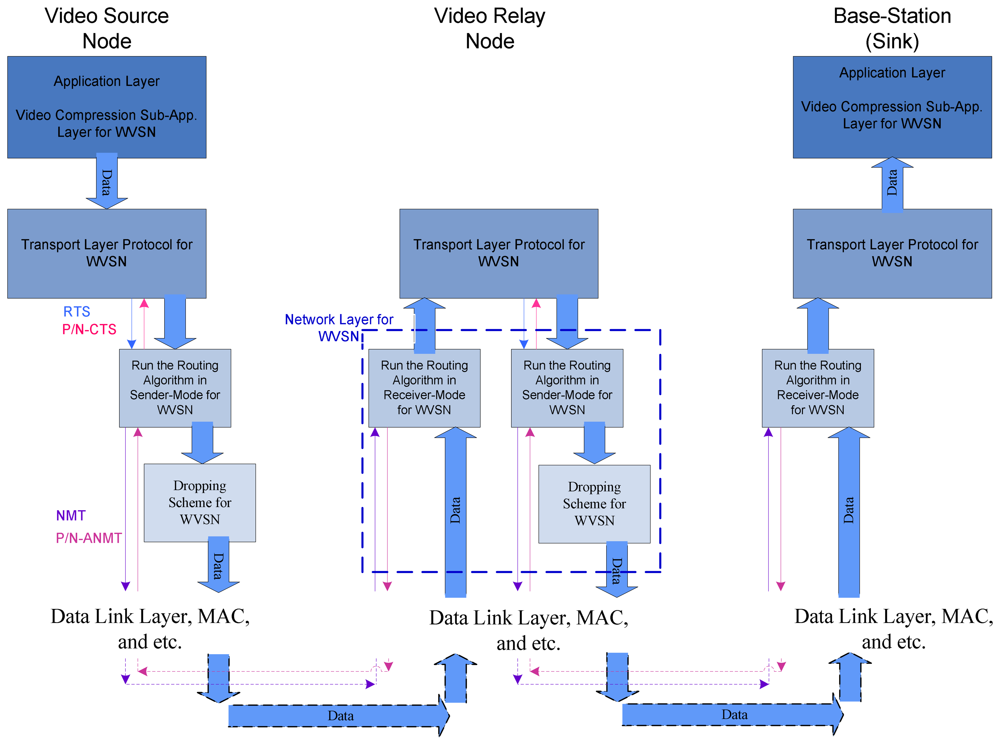
The proposed architecture provides energy efficiency and video Quality by customizing three layers of the wireless sensor networks communication protocol stack. The customized layers are application layer, transport layer, and network layer. Some new policies, algorithms, and protocols in these layers are presented. These three layers and their relations have been shown in
Figure 1, and are discussed briefly in the following subsections.
3.1. Video Compression Sub-Application Layer Protocol for WVSN
Since video requires huge amounts of data in comparison with other kinds of information, reducing its size without interfering video quality decreases bandwidth usage and increases the communication speed. Hence, in the application layer a video compression sub-layer, which consists of a new compression model that differentiates video frames and prioritizes packets, is proposed. This compression sub-layer observes major points of video transmission as far as possible. Also, it provides data with some extra information to be used in other layers. The details of video compression sub-layer are presented in Section 4.
3.2. Real-Time and Reliable Transport Layer Protocol for WVSN
For transport protocol of WMSN reliability, low delay and real-time services are the aspects involved. The proposed protocol in transport layer is aimed to meet the expectation of the concerned aspects by using information which is provided by upper layer. Transport layer protocol forwards data packets without using retransmission techniques while it takes account of reliability. In addition, this protocol provides inter-layer command messages that are used in other layers to achieve real-time transmission. Section 5 explains the proposed transport layer protocol in detail.
3.3. Routing Protocol and Innovative Dropping Scheme in Network Layer for WVSN
Network layers play an important role in delivering the multimedia from video source node to the Sink. As a result, energy-efficiency and video quality are influenced by the approaches of this layer that include routing protocol and dropping scheme. The presented routing protocol forwards packets using a hierarchical architecture topology and an adaptive single-path transmission. In used single-path transmission protocol, energy efficiency increases more remarkably than multi-path transmission protocols which were proposed previously. In this layer, a dropping scheme that causes nodes to save energy and to prolong the lifetime of the network is proposed. On the basis of energy level of each node and information that has been provided by video compression layer inside the received packet, dropping scheme decides to discard data packets. As regards the structure of the network layer, video quality is preserved while energy consumption is distributed fairly among all the nodes. Routing protocol and new dropping scheme are described more in Section 6.
4. Video Compression Sub-Application Layer Protocol for WVSN
This sub-layer, located in application layer (App.), consists of a model for compressing and transmitting video in WMSN. The proposed model is based on MPEG-2 [
34] and is called M-MPEG (Modified-MPEG). M-MPEG model provides facilities to overcome available constraints in VSNs such as bandwidth and energy. It is designed compatible with other layer services; therefore, the generated packets in this model consist of additional information which is used in the services of other layers such as proposed video transport and network layer. The user can adjust the energy consumption, video quality, and bandwidth usage in this sub-layer.
M-MPEG supposed that each video frame is in gray-scale. The resolution of video frames should be adapted to the need of each application. The M-MPEG utilizes two types of video frames. The first type is named Main-Frame (M-Frame), and second is named Difference-Frame (D-Frame). These types and their methods are described below.
4.1. M-Frame
M-Frames are compressed before transmission, using an extended JPEG method [
34]. Compared with JPEG, the extended JPEG method has an additional step that prioritizes image blocks. This step is called priority level step. Details are presented in the next sub-sections.
4.1.1. M-Frames Compression
In M-MPEG, M-Frame compression has been performed in 5 steps sequentially:
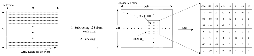
- Step 1:
128 is subtracted from each pixel of M-Frame to put zero in the middle of the range [
34]. Next, each M-Frame is divided up into 8×8 blocks without overlapping. An example is shown in
Figures 2 (a, b, and c).
- Step 2:
DCT [
35] is applied to each block independently. The output of each DCT is an 8×8 matrix of DCT coefficients as shown in
Figure 2.d.
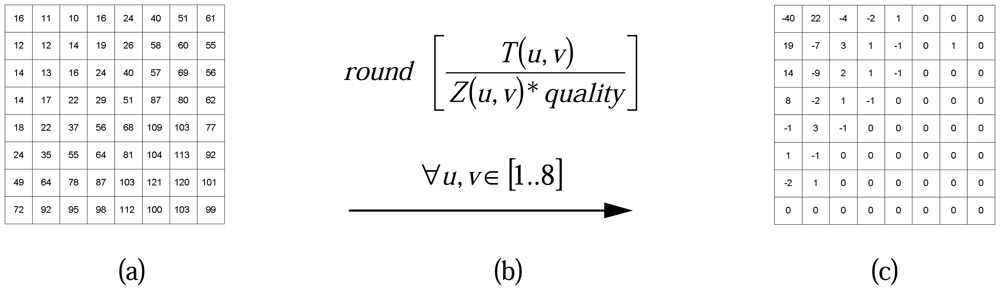
- Step 3:
In this phase that is called quantization phase; the less important DCT coefficients are wiped out using quantization matrix. To do this, each of the coefficients in the 8×8 DCT matrix (
T) is divided by the corresponding standard quantization matrix elements (
Z) [
34]. The
quality coefficient can be used to adjust compression ratio to get the expected video frame quality.
Figure 3 exemplifies this step.
- Step 4:
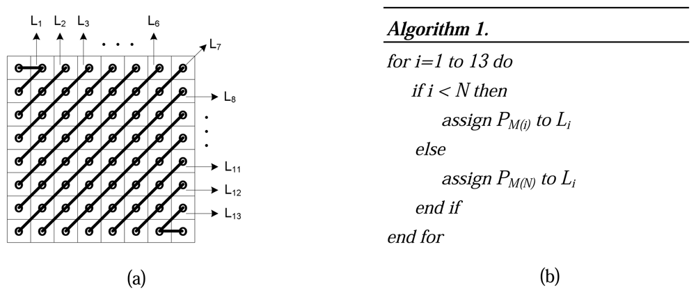
The elements of each block are partitioned into
13 levels as it is shown in
Figure 4.a. This structure is formed in order of importance of DCT quantized coefficients in each block. Also, this scheme facilitates linearization which happens in the next step. Each level has a priority that is assigned to it using the Algorithm.1 in
Figure 4.b.
In
Figure 4.b,
N defines the number of priority levels that are chosen for transmission. This value is selected by the user with regards to the constraints and specified application. It determines the amount of sent pixels, thus,
N has a direct influence on video quality and energy consumption. Since Level-1
(L1) contains a DC component and two major low frequency AC components (as shown in
Figure 4.a), it has a higher priority and, as is shown in
Figure 4.b,
PM(1) is dedicated to it. Thus, it is necessary to send the data packets with priority
PM(1) to the Sink in a more reliable way. To achieve full reliability, all communication stack layers cooperate with each other.
PM(N) is the lowest priority because the most of elements in this level are zero DCT coefficients. Data packets with priority level
PM(N) are discarded immediately because they have not great effects on video quality.
PM(2) to
PM(N-1) are assigned to the other levels from
2 to
N-1, respectively. Data packets with these priority levels are transmitted using semi-reliable policies. These policies have used different probabilities for transmitting data packets. Policies and the way in which probabilities are assigned to each level are described in Sections 6.2.
- Step 5:
The 64 elements of each block are linearized and run-length encoding is applied to the result. ZigZag transform is used to linearize block elements.
After end of these steps M-Frame data packets are transferred to the next communication layers where hop-by-hop transmission is used to deliver them to the base-station (Sink).
4.2. D-Frame
The result of subtracting current frame from M-Frame is called D-Frame. M-Frame in both receiver and transmitter is buffered until the next M-frame is transmitted. Therefore, by using a D-Frame we can construct a new video frame drawing on the buffered M-Frame at receiver end.
4.2.1. D-Frames Compression
The operations performed to transmit the D-Frame are completely different from MPEG-2. D-frame compression and transmission method is described in the following steps:
- Step 1:
D-Frame is generated as explained above. Each D-Frame is divided into 8×8 blocks.
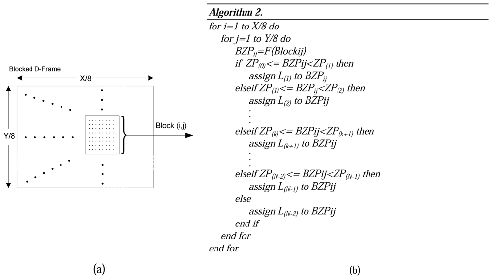
- Step 2:
The number of zero elements of each block
ij (
BZPij) is computed by using function
F(
Blockij). The maximum number of
BZP is
64, which is divided into
N equal parts with
ZP(k) and
ZP(k+1) as boundaries. A level is assigned to each block of
Figure 5.a, using Algorithm.2 presented in
Figure 5.b.
Then a priority is assigned to each leveled block using following relation:
D-Frame packets with priority level (1) (PD(1)) are very important and have the maximum number of dissimilar pixels. They should be delivered to the base-station (Sink). Therefore, M-MPEG uses highly reliable schemes to transmit this type of packets (More details are presented in next sections).
It is not necessary to transmit the packets with priority PD(N) because these types of packets have minimum number of dissimilar pixels and their transmission does not important effect in video quality. The PD(2) to PD(N-1) are delivered to the Sink by using semi-reliable policies. In these policies, each source or relay node in communication transmits the packets to the next hop employing their probabilities. Probability assignment is described in Section 6.2.
- Step 3:
In this step, run-length coding and then Huffman coding are applied to packets. Finally, packets with different priority levels are transmitted to lower layers of communication protocol stack.
4.3. M-Frame Transmission in Dynamic Periods
MPEG-2 transfers I-Frames at regular periods. Thus, it requires extra bandwidth and has high energy consumption. M-MPEG model uses the adapted period to transmit M-Frame because in the WVSNs applications camera and background are often stationary and no fast moving object exists. This idea leads to many constraints of VSNs to be observed on the part of the M-MPEG. These adapted periods are selected in accordance with variations of background that is described in the following.
The proposed adapted M-Frame transmission is based on the number of pixels that should be transmitted in M-Frame and D-frame packets. Therefore, two functions were defined to determine when an M-Frame should be transmitted instead of a D-Frame. These functions are called SPMF (Sending Pixels in M-Frame method) and SPDF (Sending Pixels in D-Frame method).
4.3.1. SPMF
This function is employed to find total number of pixels, which will be sent, with applying M-Frame compression method. It is defined as follows:
In this equation, X and Y are video frame resolution in the columns and rows of video frame respectively. PPM(i) is pixel numbers in priority level (i) of each M-Frame block, and Pi is probability of dropping data packets with priority level (i).
4.3.2. SPDF
The function is used to find total number of pixels which will be sent using D-Frame compression method. It is defined as follows:
In this equation,
BPD(i) is number of blocks with priority level (
i),
APi is the average of priority level range and
Pi is probability of dropping data packets with priority level (
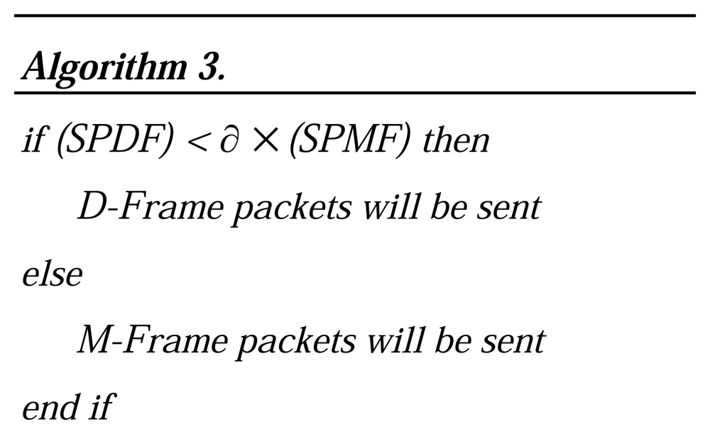
i). The Algorithm.3 in
Figure 6, is used to decide when an M-Frame should be transmitted.
In this algorithm, ∂ ∈ [0, 1] is a coefficient that affects energy saving and video quality. Using a lower value of ∂ leads to M-Frame being sent to a high frequency, which results in more energy and bandwidth consumption. It causes, however, better video quality. Higher values of ∂ causes lower video quality and more energy and bandwidth saving.
5. Real-Time and Reliable Transport Layer Protocol for WVSN
In this article, a new transport layer protocol is designed to satisfy constraints of video sensor nodes and required QoS in video transmission. To support data packets that are generated by video compression sub-layer, priority-based-transport services are provided. New transport layer protocol which is called real-time and reliable video transmission transport layer protocol utilizes upper layer information to provide these services.
To achieve real-time video transmission, proposed video transport protocol does not retransmit data packets. Instead some methods are employed to satisfy the reliability as a substitution. The M-Frame and the first priority level of D-Frames as mentioned in Section 4.2 are the most important data in video transmission. Therefore, transport protocol endeavors frequently to establish a connection for transmitting first priority level of M-Frames. In other priority levels, M-Frame take precedence over D-Frame in the same priority levels. Moreover, it is suggested that data link layer applies reed-Solomon forward error correction [
36] to M-Frames and first priority level of D-Frames. In the following, new protocol transmission operations are discussed in two phases.
Negotiation with Network Layer phase
In this phase, video data frames have been received from sub-application layer (in the case that current node is the capture video node) or network layer (in the case that current node is a relay node). Then, received video frames are extracted in order of priority. For delivering each priority level in a reliable way, three inter-layer command messages are used between transport and network layers: Request To Send (RTS) and Positive/ Negative Clear To Send (P/NCTS).
RTS is used to notify the network layer that there is data with selected priority level of a frame to be sent. RTS contains the type of the frame and priority level of the data. Connection is established separately for each priority level of frames. Before forwarding the whole data of the priority level, an RTS must be sent to every priority level to achieve real-time video transmission.
The RTS response is CTS that network layer forwards to transport layer. The CTS command message contains a positive or negative flag which notifies transport layer of the ability of the network layer to transmit data. The PCTS means that a valid path exists for the selected priority level and NCTS shows the opposite.
In case PCTS is received from network layer, data transmission continues with
Data transmission phase. Otherwise, type of frame and priority level defines next step as following:
Priority level (1) of M-Frame: In this case, if the Number of Retransmissions (NoR) is less than a threshold, another RTS is retransmitted for current priority level to the network layer. Otherwise if NoR passes the threshold; VSN goes to sleep-mode.
Other priority levels of M-Frame: Whole data of current priority level is discarded, and if any other priority level exists in this frame, another RTS is sent for next priority level. In the case that, no other priority level exists, RTS is sent for the first priority level of the next frame. In other cases transmission continues in accordance with the received CTS.
D-Frame: Regardless of priority level, whenever NCTS is received for priority level of D-Frame the entire frame is dropped and negotiation is started for next video frame.
Data Transmission phase
By receiving the PCTS, network layer shows that it finds proper parent for forwarding the specified priority level. Therefore entire data of selected priority level is transmitted bursty through network layer. After data transmission is completed, negotiation is started for next priority level. If sent priority level is the last priority level of the current frame, transmission proceeds to Negotiation with Network layer phase for next video frame.
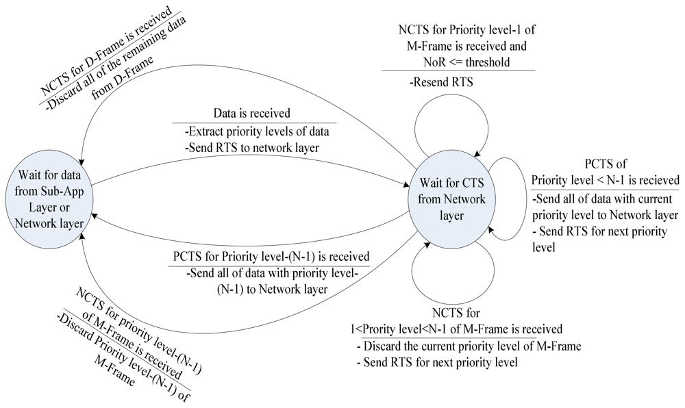
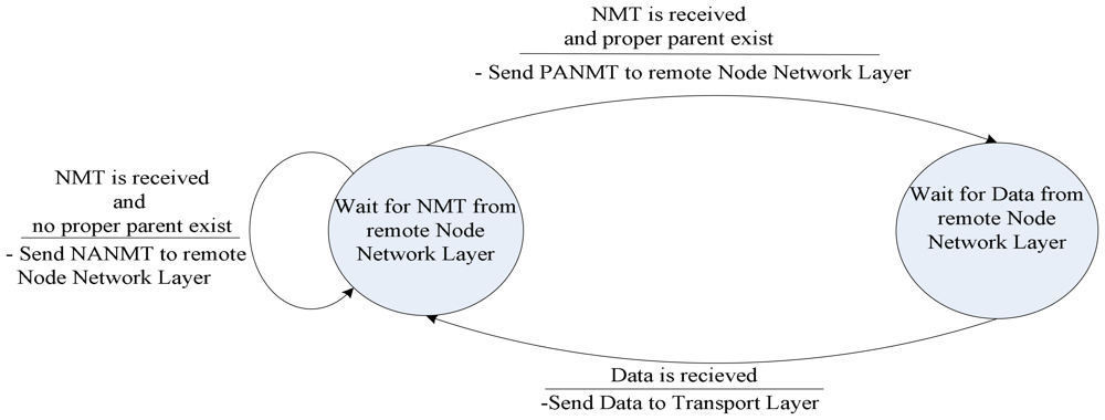
For implementing the proposed transport protocol, a simple state-machine is suggested. In order to describe the operations of the transport protocol two waiting states are presented in the state-machine. The conditions of switching between states beside tasks of each transport protocol phase are mentioned on the edges as shown in
Figure 7.
As regards the fact that RTS can be sent to first priority level of M-Frames several times, if it exceeds the threshold –as was mentioned above– transport layer goes to sleep-mode and notifies networks layer in receiver-mode (relay node) or sub-application layer (source node). Also, when the network layer sender assures that no parent is available for transmission, regardless of the number of RTS retransmission, it forces transport layer to be in sleep-mode. Transport layer stays in sleep-mode until hierarchical network topology is reconfigured (see Section 6.1).
6. Network Layer for WVSN
The proposed network layer provides two services: single-path routing protocol and dropping scheme. Proposed routing protocol finds a single-path adapted with nodes status (energy and topology) and data importance for video transmission. Dropping scheme is a policy for reducing bandwidth and energy consumption of nodes without compromising the quality of services such as video quality. This scheme works by dropping low priority packets with regard to node-Sink distance. Single-path video routing is provided using inter-layer/inter-node command messages which are received from transport layers and negotiating with remote node. Dropping scheme is provided by using information embedded in data packets in compression sub-application layer and routing protocol like priority level of the data and hierarchy level of the capture node.
6.1. New Energy-Efficient and Single-Path Routing Protocol for WVSN
The main task of wireless sensor nodes is to sense and collect data from a target domain, process the data, and transmit the information back to the base-station (Sink) in all applications. Therefore, development of energy-efficient routing protocols is necessary to set up paths between sensor nodes and the Sink. In addition, to use this protocol in wireless video-based sensor networks, it should provide high quality video transmission.
The proposed routing protocol is a single-path routing based on hierarchical network topology. In EQV-Architecture, a Hierarchical Data Aggregation scheme for sensor networks (HDA) [
37] is utilized for configuring hierarchical topology. The routing protocol supposed that in each time Sink requests to receive a specified video from the source node only, and the aim of routing is to find an energy-efficient single-path from the source node to Sink while preserving video quality. This protocol is called Energy-efficient Single-path Routing Protocol.
The proposed routing protocol consists of two kinds of tables: Priority-Table (Pr-T) and Parent-Table (Pa-T). Pr-T is an
N-1 cell array that
i-th cell content shows the parent which can forward packets with
i-th priority level.
N is the maximum priority level that is defined by user in compression layer. As was mentioned in Section 4, only data with priority (
1) to (
N-1) will be transmitted. Every time after reconfiguring the hierarchical network structure, cells of Pr-T are set to zero. This table is shown in
Figure 8 in detail.
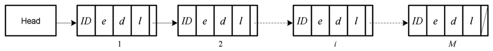
Pa-T is a link list data structure that includes information that a child has about status of its parents. The fields of each node of link list are: parent
ID, energy (
e), distance (
d) and also the minimum priority level (
l) that this parent can transmit as is shown in
Figure 9.
When hierarchical structure of the network is reconfigured, in addition to required information for constructing hierarchical tree, each node sends some data to its children to update their Pa-T. Using this information, fields of Pa-T are filled with updated energy, distance, and minimum priority level values of parents. The priority level value that each node transmits to its children is the result of the following equation:
Where Pk -1 is the maximum priority level that its current parent is able to transmit, and it is computed on the basis of node energy independent from situations of other nodes. The computation method of Pk is explained in Section 6.2.1. Pi stands for priority level that the parent i in Pa-T list of current parent can transmit and M is the number of the node's parents.
In the proposed routing protocol, Pr-T and Pa-T need more memory than does the conventional routing protocols. Unlike energy, memory is a reusable resource. Therefore, it is reasonable to use a little more memory for achieving energy efficiency.
Depending on whether the proposed routing protocol is in sender-mode or in receiver-mode of the VSN, it works differently. Two dissimilar algorithms for mentioned modes are defined below.
6.1.1. Routing protocol for Sender-Mode of VSN
In order to forward the received data in transport layer to next hop in a reliable way, the proposed single-path routing protocol goes through sender-mode phases as is delineated below:
Parent Selection phase
This phase begins when an RTS is received from the transport layer. An appropriate parent is chosen by drawing on Pr-T and Pa-T in accordance with priority level which was mentioned in RTS. If any value other than zero exists in cell of Pr-T pointed to by priority (l) (Pr-T [l]), the value shows the relevant parent ID. Node selects this parent as a node to communicate with. In a case that Pr-T [l] content is zero, algorithm refers to Pa-T. Considering the parents which Pa-T[l] has the lowest priority level, the most appropriate parent according to energy and distance is selected by computing the value of f(e,d). Therefore, the parent with maximum value of f(e,d) is chosen and the ID of the chosen parent will be put in all zero cells of Pr-T and Remote Negotiation phase begins. If no acceptable parent exists in Pa-T, NCTS is sent as a notification to the transport layer and the algorithm waits for another RTS from Parent Selection phase.
In order to distributing the energy consumption in the network and having fair energy management,
e is used as the major factor for parent selection, and
d is taken in to account to decrease hop-by-hop delay. Therefore,
f(e,d) is defined as
e2/d. Also, some other literatures deployed energy and distance as two parameters for choosing next hop node as well in similar manner [
38] and [
39].
Remote Negotiation phase
Three inter-node command messages are utilized for negotiating with remote node (selected parent) in transmission. After selecting a proper parent a message called Negotiation Message for Transmission (NMT) is forwarded to the selected parent. Next operation of routing protocol is influenced by Answer to NMT (ANMT) which could be positive (PANMT) or Negative (NANMT). Three conditions could occur at this stage:
Receiving PANMT: In this case, a PCTS is forwarded to transport layer to notify it and routing continues from Preparing Data for Remote Transmission phase.
Receiving NANMT: Both Pa-T and Pr-T are updated by receiving NANMT. Priority field of selected parent in Pa-T is updated with value of priority level field of NANMT. Pr-T also changes; all cells with the ID of selected parent are set to zero. Also, NCTS is sent to transport layer and routing proceeds from Parent Selection phase.
Timeout: When selected parent does not respond to NMT in a specified time interval, the timer times out; then Pa-T and Pr-T become updated. Selected parent is eliminated from PaT and also all cells of Pr-T which contain the ID of this parent are revalued to zero. Moreover, NCTS is forwarded to transport layer and routing starts from Parent Selection phase.
Preparing Data for Remote Transmission phase
In this phase, data is received from transport layer and is put through dropping scheme (see Section 6.2.). Then, all data from current priority level is forwarded to the selected parent bursty. The routing is started from Parent Selection phase after sending entire data to remote parent.
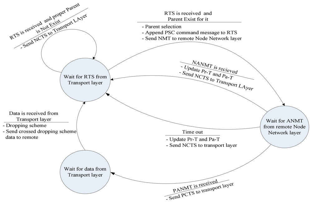
Figure 10, shows a three-state state-machine which is used to reveal routing protocol in sender-mode. In this state-machine, conditions and operations are laid at the edges.
Assuming the condition that no parent exists in Pa-T, routing protocol in sender-mode notifies transport layer and goes to sleep-mode. Whenever hierarchical network topology is reconfigured, routing protocol changes its mode and starts from Remote Negotiation phase.
6.1.2. Routing protocol for Receiver-Mode of VSN
Checking for Proper Parent phase
When NMT is received from the remote node, routing protocol responds to it either by PANMT or NANMT depending on its energy status and Pa-T. In a case that it has a suitable parent it responds by PANMT and goes to the next phase. Otherwise, the priority level field of NANMT should be filled using the result of
Equation 4. Then NANMT is forwarded to remote node and routing waits for another NMT.
Receiving Data phase
In this phase, whole data of the same priority level is received and delivered to transport layer. The routing operation begins from Checking for Proper Parent phase.
Routing protocol in receiver-mode also can go to sleep-mode under specified condition. When transport layer is in sleep-mode it also notifies routing protocol to go to sleep-mode and not to respond to NMT. Routing protocol in receiver-mode keeps on routing whenever hierarchical network topology is reconfigured. The operation of routing protocol in receiver-mode is clarified by the state-machine in
Figure 11.
6.2. Dropping Scheme
Dropping process consists of two stages; at the first stage, each node decides which priority level should be sent and at the second stage each node drops some packets randomly while taking account of the priority level of the packets and distance between current node-Sink.
6.2.1. Energy Aware Dropping
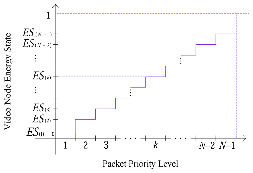
Clearly the energy of each active video node decreases over time. Therefore, discarding priority level is calculated on the basis of normalized energy level of a node. All received packets with this priority level and lower are discarded. As shown in
Figure 12, each priority levels
P1, P2, …, Pk, …, PN-1, is associated with a normalized energy level
ES(1),
ES(2), …,
ES(k), …,
ES(N-1) respectively. These levels should be specified by the user regarding to the application.
Pk stands for both
PM(k) and
PD(k) as mentioned in Section 4.1.1 and 4.2.1, respectively and for each priority level (
k) ∈ N, there exists
ES(k) ∈ [0,1) such that
ES(k) <
ES(k+1). For example, if energy of a node becomes less than
ES(k), then packets with priority level (
k) and lower priority levels are not transmitted.
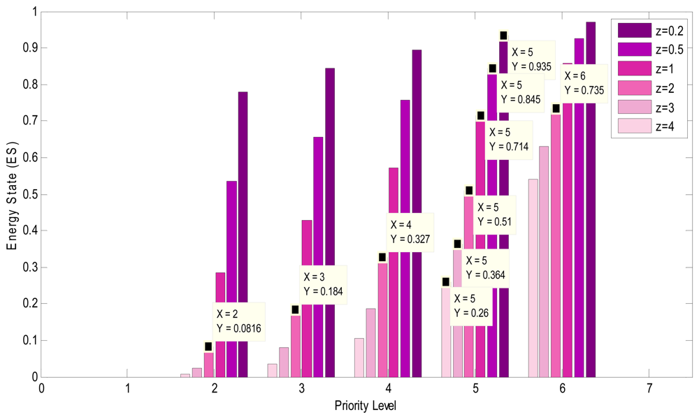
In order to reach a proper energy level for each priority level that is compatible with the requirement of application as well,
Equation (5) is suggested:
In this equation,
N is the maximum number of priority levels and (
l) is the current priority level.
z is used to make
Equation (5) adaptable with different applications. For instance, if in an application, lifetime of the network is the major point and normal video quality is sufficient, choosing
z <
1 in the equation will lead to high values for
ES(l). Consequently, nodes start to drop priority levels more quickly. Therefore, video quality decreases when lifetime of network improves significantly. Conversely, for applications whose concerning point is video quality, values greater than
1 for
z causes nodes to begin dropping in lower level of energy. In all simulations
z is considered
2.
Figure 13, shows different
ES(l) calculated for various values of
z.
The energy-aware dropping scheme uses
Equation (5) to define the priority level which can be sent. This scheme first maps the domain of the nodes energy between
0 and
1, and then calculates the result of
Equation (5) according to current priority level (
ES(l)). After comparing the mapped energy with
ES(l), it will be determined whether or not this priority level can be transmitted. If mapped energy of the node is greater, node is allowed to send the data of the priority level; otherwise the node is unable to send the priority level. For example by choosing the value
2 for
z in
Figure 13, if a mapped energy of a node equals
0.4 then
ES(4) is
0.327 for data packets with priority level (
4). In this example since
ES(4) is less than mapped energy, node passes them to the next stage. Unlike for priority level (
5) which calculated
ES(5) is
0.5, the node drops packets.
If a node cannot transmit packets with specific priority level and lower than that, its child is not allowed to send packets with this priority level and lower to this node. The node notifies its children by ANMT when they ask for communication. If all parents of a node cannot send packets with specific priority level and lower, that node itself cannot send packets as well.
6.2.2. Random Early Dropping
Some packets are dropped before arriving at energy aware dropping so that the quality of video is still satisfactory. Applying random early dropping to data packets which are not dropped in energy aware dropping also helps increase the lifetime of the network. Early dropping of the data packets occur on the basis of node energy and hierarchical level with considering the priority and influence of these packets on video quality. Packet selection for early dropping consists of two phases: energy level and hierarchical level. All packets selected in both energy level and hierarchical level selection phases are early dropped. In the following, two packet selection policies are described.
A. Energy level based packet selection
This selection benefits from video compression layer prioritization. The probability that a packet is dropped depends on the priority level of the packet and energy level of the node. The packet with first priority level never drops.
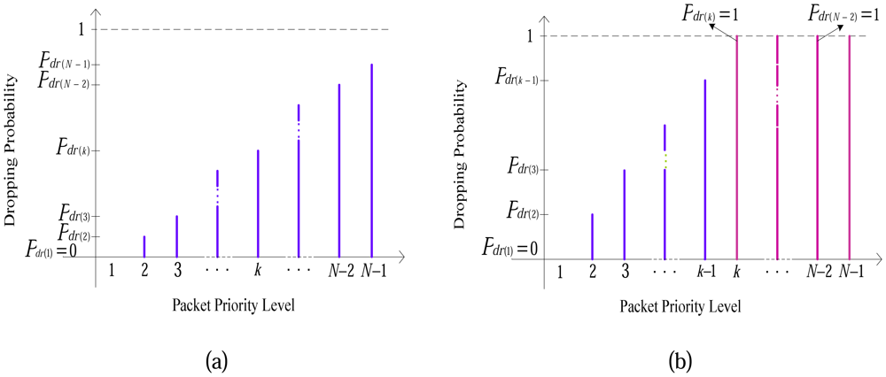
Dropping probabilities Pdr(1), Pdr(2), …, Pdr(k),…, Pdr(N-1) are assigned to each priority level P1, P2, …, Pk, …, PN-1 respectively. Where Pk stands for both PM(k) and PD(k) and for all (k) ∈ N, Pdr(1)=0, Pdr(k) ∈ [0,1]. Since the content of packets with priority level (k) is most important than content of packets with priority level (k+1) then Pdr(k)<Pdr(k+1).
Furthermore, the values of dropping probabilities and energy state of the node have negative correlation in a way that when battery level decreases, dropping probability increases. When the energy level of a node is more than
ES(N-1) (node has enough energy) the packet is selected with probability as shown in
Figure 14.a. When the energy decreases to less than
ES(k) the dropping probability increases as shown in
Figure 14.b. The selection probability is constant between two consequent normalized energy levels and changes when it passes an energy threshold level (as has been shown in
Figure 12).
The packet selection probability function can be defined with regards to application requirements. The function used for probabilities calculation should have a domain based on priority levels that node is allowed to send, and range between
0 and
1. Also, it should be strictly increasing. The suggested function is:
In this equation,
Pdr(l) is the dropping probability for packet with priority level (
l),
Pk is the maximum priority level that VSN can transmit see Seccion 6.2.1,
l is the priority level of current packet, and
β is a coefficient which improves the flexibility of the
Equation (6) which is defined between [0, 1]. After specifying dropping probability (
Pdr) for each packet, a random number
R selected from [0, 1], if
R<=
Pdr(l) packet is eligible for dropping, otherwise the packet is transmitted.
B. Hierarchical level based packet selection
In an energy level based scheme, the probability of discarding a packet is independent from the number of nodes that packet passed. Dropping a packet that is close to Sink (passed a lot of nodes) wastes more energy than dropping a packet close to the source node (only a few nodes passed) does. Thus, it is unfair to drop packets only on the basis of node energy. Consequently, an efficient packet discarding policy should consider preceding invested energy of each node. To achieve same drop probability for all packets (with the same priority level) received in the Sink, which originated from any node of the network, a fair drop selection policy should be defined. This motivates to find another probability factor to modify energy based drop probability. Therefore, the following equations should be satisfied:
In these equations,
is the probability of receiving a packet in the base-station (Sink), where
l is the number of levels that a packet should pass,
k is packet priority level,
a is the relying video node level,
b is the source video node level, and
λ is the constant that shows the specified dropping probability. It is optimistic to have functions that generate the related probabilities in the mentioned equations. Therefore, a close function is defined to calculate a probability that in conjunction with energy based packet drop probability results in a reasonable fair drop probability that somehow satisfies
Equation (7). The proposed four-variable function is presented in
Equation (8).
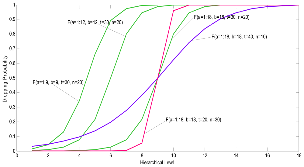
The presented function gives the second drop probability of each packet. In this equation t and n are two positive constant values that should be specified with regards to application. Both a and b are related to hierarchical levels (see Section 6.1. above) of relay and video capture node respectively.
Using this probability function along with energy based dropping probability, increases the receiving chance of the packets which passed more nodes than others. In other words, the receiving chance of packets generated by nodes close to the Sink is somehow the same as packets generated by nodes far from the Sink.
To drop a packet, a random number
R ∈ [0, 1] is chosen. In case of
R =<
F (a, b, t, n), the received packet will be dropped if it has energy based dropping condition, otherwise the packet is forwarded.
Figure 15, illustrates the effect of some parameters on the function
F(
a,
b,
t,
n) at a network with
18 hierarchical levels.
7. Simulation
The performance of proposed architecture was evaluated by MATLAB using Communication Toolbox and Video and Image Processing Block-set. Also, the required functions are generated by M-Files. The hierarchical network topology had
18 levels and
1000 video sensor nodes. All sensor nodes are considered homogeneous and their energy is supplied with two
1.5 V batteries. The video resolution is
320×240. To perform the simulation it is assumed that all nodes have full battery, i.e., more than
ES(N-1). The parameter
∂ in algorithm 3 is set to
0.5 and the retransmission threshold value is
3. Also in
Equation 5 the parameter
z is set to
2, in
Equation 6 the coefficient
β is
0.5 and in
Equation 8 the parameters
t and
n are set to
30 and
20, respectively.
Moreover, Energy-Efficient and High Throughput MAC Protocol for Wireless Sensor Networks (ET-MAC) [
40] is used in data link layer for simulations. In order to get precise results from the simulations the parameters of CC2420 [
41] Chipcon transceiver listed in
Table 1, were used.
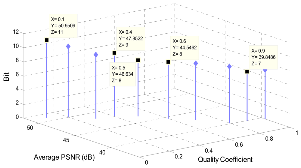
7.1. Selecting Quality Coefficient
The
quality coefficient parameter affects the value of each element in quantization luminance matrix [
34]. As mentioned in Section 4.1, an M-Frame block is prepared for transmission by dividing blocked DCT matrix with the quantization luminance matrix. Hence,
quality influences the value of each pixel in M-Frame blocks. Choosing an appropriate value for
quality coefficient is so important, since small value for it leads to a greater number of bits required for transmitting the data of each block pixel. On the other hand, high value for
quality results in a greater number of zeros in each M-Frame block. This means more data loss in M-Frame compression method. As a result, defining
quality coefficient encounters the bit-loss trade off.
The approach used for defining
quality is examining different values for it. By analyzing average Peak Signal-to-Noise Ratio (PSNR) [
42] and required bit in different
qualities in various video frames, it is shown that some
quality values require
8 bits for transmitting each pixel of M-frame blocks. Since
8 bits are earmarked for each pixel, the value with negligible loss (proper PSNR) is selected. As
Figure 16 shows,
0.5 is the best value for bit-loss trade off which also used in our simulations.
7.2. Selecting Maximum Priority Level
The parameter
N is the number of priority levels which are selected for transmission. Each one of the mentioned priority levels includes some pixels of a frame. High values for
N result in forwarding a large number of pixels for M-Frame blocks. This causes increase in energy consumption and bandwidth usage, as well as improvement in video quality. On the other hand, transmitting few priority levels has opposite consequences. Comparing the average PSNR and pixels for all values of
N from
1 to
13, we concluded that
7 is an acceptable value for
N and this value is used in simulations.
Table 2, contains these results.
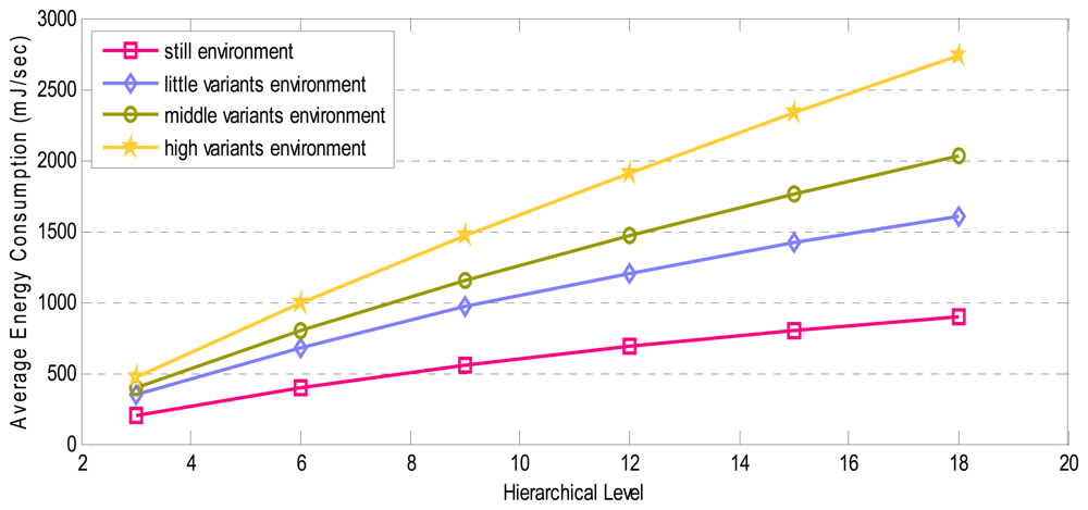
7.3. Analyzing Energy Efficiency and Video Quality for Different Environments
In this section, we evaluated the performance of presented architecture. The behaviors of designed architecture should be considered with the aim of having actual results for our simulation. As mentioned in Section 4.3, the period of forwarding M-Frames depends on the number of the pixels which are used for delivering M-Frames and D-frames. Moreover, priorities assigned to D-Frame blocks are related to the difference between pixels of current D-Frame and saved previous M-Frames. Thus, the performance of the architecture is associated with the variation degree of the environment. Owing to this fact, examined environments are divided into four categories: still environment, little-variant environment, middle-variant environment, and high-variant environment. The performance is calculated in each of these categories.
In the following, the average result of five video samples captured by video nodes located in hierarchical levels from
3 to
18 during
10 seconds in each environment is presented.
Figure 17, shows the relation between the energy consumed and hierarchical levels for tested environments. Having analyzed simulation results, we concluded that energy consumption depends on the variants in the examined environment. When variation degree of the environment increases, M-Frames are forwarded with higher frequency because of more different pixels between captured frame and saved M-Frame. This leads to more pixels of D-Frames to be sent. Consequently, the average energy consumption increases and high-variant environments consume more energy in comparison with other environments (as shown in
Figure 17).
Also, the level of the source node in the hierarchical topology influences the energy consumption of the whole network. Since the location of the source node determines the number of contributed intermediate nodes in delivering video frames, energy consumption increases when number of relaying nodes grows.
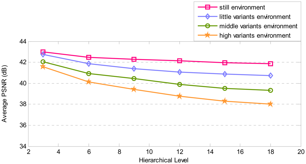
Another factor to be analyzed is video quality which is inspected by average PSNR.
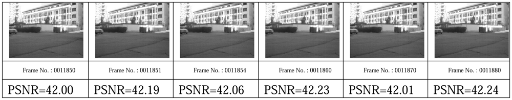
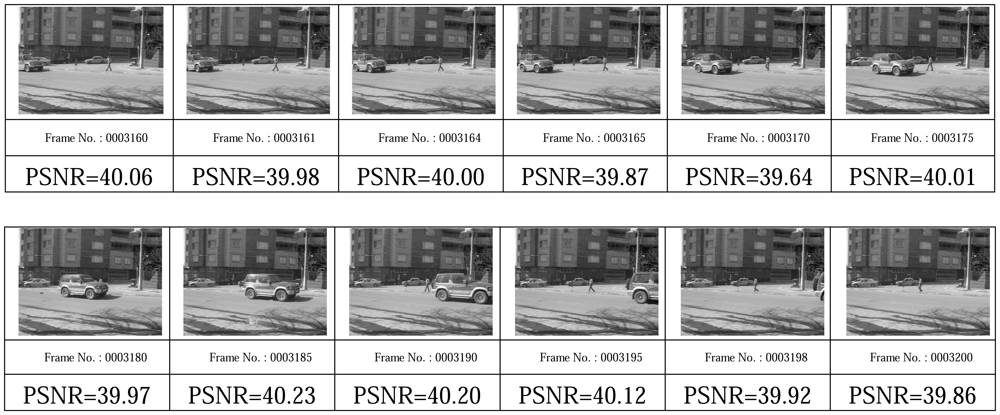
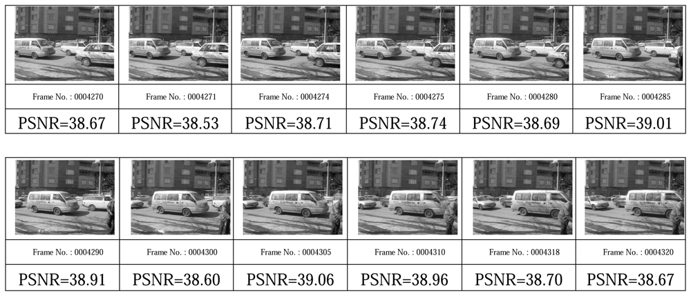
Figure 18, elucidates the correlation between average PSNR and hierarchy level. Average PSNR changes in associated with variants in the environment and hierarchy level of video source node like consumed energy. The major reason of this fact is the impacts that dropping scheme has on average PSNR. In high-variant environment, more pixels change; thus, sending more pixels for a frame is needed. Therefore, on the same probability of packet dropping, more pixels of the frame are dropped through transmission and smaller number of frame's pixels is received in Sink. As a result, average PSNR is lesser than other categories of environments. Interpretation of the result of simulation in EQV-Architecture shows satisfactory functionality.
Figures 19,
20,
21, and
22 show some video frames from different categories of environments with their PSNRs in receiver side. These frames are samples that were used to calculate average PSNRs in
Figure18.
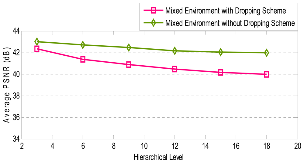
7.4. Effect of Random Early Dropping Method on Energy and Video Quality
Random early dropping is presented in Section 6.2.2 as an approach for extending the lifetime of the WVSN. Although this scheme has various benefits, it influences the video quality. In this section, two criteria are utilized for evaluating the performance of dropping scheme. The criteria are average bytes which are forwarded from source to Sink and average PSNR in receiver side. Video is transmitted first by using dropping scheme and then without using this scheme. It is assumed that all nodes have full batteries and the environment examined is a mixture of all four categories of environments. Furthermore, simulation lasted for 10 seconds.
The simulation results shown in
Table 3, are evidence that the number of sent bytes in dropping scheme decreases. According to
Equation (9), the optimization of the sent bytes in the dropping scheme is
24%.
In this equation, i is the hierarchical level that video capture node is situated on.
On the other hand,
Figure 23 shows that average PSNR is reduced by approximately
1.51 dB. The resulted value, however, is a satisfactory average PSNR for video transmission. Based on the achieved results, it is reasonable to use dropping method for achieving energy efficiency. Dropping scheme takes account of energy and hierarchical levels of nodes and data importance for dropping. Therefore, it drops low-priority data while having in view the level of source node. In short, average PSNR does not change a lot even when about one quarter of the data is dropped.
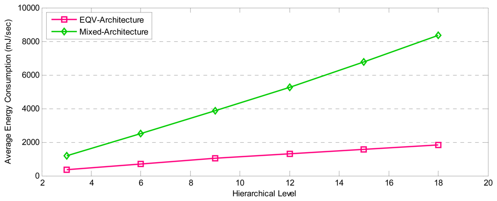
7.5 Comparing EQV-Architecture with Other Protocols
In order to evaluate the EQV-Architecture effectively, it is compared with another architecture composed of three different protocols. In the set of selected protocols, there were protocols compatible with real-time transmission and multi-path routing. The chosen protocols were: MPEG-2 in application layer, MRTP [
24] in transport layer, and MMSPEED [
31] in network layer. The simulation performed in 5 sample of mixed environment.
Figure 25, shows the comparison of average energy consumption in these two architectures. EQV-Architecture saved more energy than Mixed-Architecture does. That is due to the fact that Mixed-Architecture sends I-Frames periodically [
34] and delivers packets in multi-paths, while EQV-Architecture utilizes dynamic period for transmitting M-Frames in single-path hand in hand with dropping scheme. Therefore, EQV-Architecture saves approximately
75% of energy.
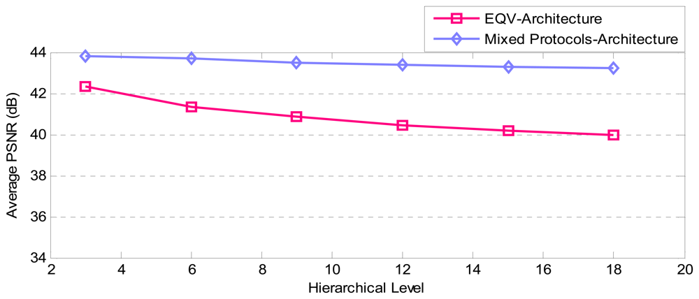
Another point for comparison is video quality based on average PSNR which is illustrated in
Figure 26. It shows that however EQV-Architecture provides less PSNR than Mixed-Architecture, the resulted PSNRs are satisfactory.
8. Conclusions
In this article the EQV-Architecture for video transmission in wireless multimedia sensor networks is presented. Battery awareness and video quality issues are considered in application, transport and network layers of communication protocol stack. A prioritized video compression protocol in application layer and new transport layer protocol along with two dropping schemes and single-path routing protocol in network layer are introduced in this architecture. The algorithms, methods, and protocols presented here are in accordance with WVSN and support two mentioned issues.
Simulation for presented architecture is applied in various environments with different variants from the perspectives of both energy-efficiency and video quality. Simulation results indicate that the optimization of energy consumption and also video quality in proposed architecture differ in disparate environments, but this architecture has better performance than other conventional architectures. In other words: EQV-Architecture extend the lifetime of the networks while providing sufficient video quality. In the future, architecture with ability to correspond multi-video requests from Multi-Sinks will be investigated.


