LQER: A Link Quality Estimation based Routing for Wireless Sensor Networks

State Key of Industrial Control Technology, Zhejiang University, Hangzhou 310027, P.R.China
*
Author to whom correspondence should be addressed.
Sensors 2008, 8(2), 1025-1038; https://doi.org/10.3390/s8021025
Submission received: 11 January 2008
/
Accepted: 11 February 2008
/
Published: 15 February 2008
(This article belongs to the Special Issue Energy Efficiency and Intelligent Signal Processing for Wireless Sensing)
Abstract
:Routing protocols are crucial to self-organize wireless sensor networks (WSNs), which have been widely studied in recent years. For some specific applications, both energy aware and reliable data transmission need to be considered together. Historical link status should be captured and taken into account in making data forwarding decisions to achieve the data reliability and energy efficiency tradeoff. In this paper, a dynamic window concept (m, k) is presented to record the link historical information and a link quality estimation based routing protocol (LQER) are proposed, which integrates the approach of minimum hop field and (m, k). The performance of LQER is evaluated by extensive simulation experiments to be more energy-aware, with lower loss rate and better scalability than MHFR [1] and MCR [2]. Thus the WSNs with LQER get longer lifetime of networks and better link quality.
1. Introduction
Recent technology developments on low-power and low-rate wireless communication, micro-sensor, microprocessor hardware etc., have made wireless sensor networks (WSNs) one of the dominant research trends in the last few years. It can be potentially applied in target tracking, habit monitoring, environment observation, structural detection, physiological tele-monitoring and even drug administration, etc. [3][4][5][6][7]. To enable high performance of WSNs, there exists a number of challenges in research as well as in practice due to its wireless nature, node density, limited resources, low reliability of the sensor nodes, distributed system architecture and frequent mobility. These issues are different from those of classical wireless ad hoc networks [6][8]. The above characteristics result WSNs in an unreliable and unpredictable behavior. Therefore, Quality of Service (QoS) supporting such as data reliable transmission is actually as a big challenge as energy efficiency for WSNs.
However, current research works on routing algorithms mostly focused on protocols that are energy aware to maximize the lifetime of network, scalable for large number of sensor nodes and tolerate to sensor damage and battery exhaustion. But there are many applications including real-time mobile target tracking in the battle environments and emergent event triggering in monitoring applications etc, which require not only energy-efficient but data-reliable routing. So the dynamics and loss behavior of wireless connectivity poses major challenges to the low-power radio transceivers found in WSNs and raises new issues that routing protocols must address.
In this paper, a dynamic windows concept (m, k) is introduced to capture the historical link states and estimate link quality before routing decision making. A link quality estimation based routing estimation based routing protocol (LQER) protocol is designed, which creates a connectivity graph based on minimum hop count field and (m, k). Our proposed protocol considers both energy and link quality to avoid poor link connectivity and reduce the possibility of retransmissions. Therefore, the lifetime of WSNs can be prolonged and an improved data reliability is obtained.
The remainder of this paper is organized as follows. Section 2 introduces some related work including typical routing protocols. In section 3, LQER protocol is designed in detail, which includes dynamic windows concept (m, k), link quality estimation based on (m, k), minimum hop field establishment and description of LQER Protocol. Section 4 does the simulation experiments based on WSNsim environment that is developed by us and evaluates the performance of LQER. Finally, we make some concluding remarks and outline some future work.
2. Related Work
The growing interest in WSNs and the continual emergence of new techniques inspired some efforts to design communication protocols for this area. Communication protocols take the task of data transmission in the large scale network and are important to achieve possible better performance. Normally, current routing can be typically classified into four main categories, namely data-centric protocols, hierarchical protocols, location-based protocols and flow-based and QoS-aware protocols [9]. Of course, there are also some hybrid protocols that fit under more than one category.
The typical data-centric routing protocols proposed for WSNs include SPIN [10] and Directed Diffusion [11], which are obviously different from traditional address-based routing; location-based protocols such as MECN [12], GAF [13] and GEAR [14] require location information for sensor nodes, which are energy-aware. Hierarchical protocols are scalable for a larger number of sensors covering a wider region of interest, which overcome the defects of single-gateway architecture. LEACH is one of the first hierarchical routing approaches for WSNs [15].
Although the above three categories are promising in term of energy efficiency, more attentions should be paid to address the issues of network flow and QoS posed by real-time applications[16]. One of the protocols for WSNs that includes some notions for QoS in its routing decisions is the Sequential Assignment Routing (SAR) [17]. The SAR protocol creates trees routed from one-hop neighbor of the sink by taking into account the QoS metric, the energy resource on each path and the priority level of each data packet. By using created trees, multiple paths from sink to sensors are formed. One of these paths is selected according to the energy resources and achievable QoS on each path. Akkaya et al extend SAR by selecting a path from a list of candidate paths that meet the end-to-end delay requirement and maximizing the throughput for best effort traffic [18]. Their protocol does not require sensors involved in route setup so that the overhead problems in SAR approach can be avoided.
Minimum cost forwarding protocol is a kind of flow-based routing protocol [19]. It aims at finding the minimum cost path in a large scale sensor networks, which will be simple and scalable. The data flows over the minimum cost path and resources on the nodes are updated after each flow Ye et al also propose a cost field based protocol to Minimize Cost forwarding Routing (MCR) [2]. In the design, they present a novel backoff-based cost field setup algorithm that finds the optimal cost of all nodes to the sink with one single message overhead at each node. Once the field is established, the message, carrying dynamic cost information, flows along the minimum cost path in the cost field. Each intermediate node forwards the message only if it finds itself to be on the optimal path, based on dynamic cost states. Ma et al improve the cost field based protocol and proposed minimum hop field based routing (MHFR) protocol [1]. This protocol can be used in large scale sensor networks and ensure that the data is forwarded along shortest path and message number is least. Simulation experiments validate the effectiveness of the design.
The proposed protocol in this paper is inspired by the approach in [2] and [1]. In the proposed protocol, a connectivity graph based on hop count field is built and the concept of dynamic window (m, k) is introduced to well estimate link quality before making routing decisions. The idea of link estimation has been studied by Woo et al. in [20]. They designed and evaluated different link estimators and find WMEWMA (Window Mean with Exponentially Weighed Moving Average) is the best one for WSNs. However, it might be too complicated for resource-constrained sensor nodes to be used for routing decision. So the simple historical status of data packet is record according to (m, k), which means that if m data packets out of window k data packets in the same network flow successfully transmission to ensure adequate QoS. The link table only records historical k states and can be updated dynamically with a low computing cost and complexity.
3. Link Quality Estimation Routing Protocol Design
LQER protocol makes path selecting based on historical states of link quality after minimum hop field is established. Firstly, dynamic window concept (m, k) is presented to evaluate link reliability in subsection 3.1, and then subsection 3.2 describes how to establish minimum hop field. The path selecting of proposed LQER is described in detail in subsection 3.3.
3.1. Dynamic Window Concept (m, k)
(m, k) is firstly proposed in [21], which is a sliding window with length k to record historical states of data. It is designated Σ as the alphabet {0,1}. Σ+ denotes the sequences of length greater than 0. Σk(k > 1) denotes the sequences of length k. For a given sequence ω, the notation l(ω)=k is to denote the length of ω ∈ Σ+. Additionally, lα (ω)=m, α ∈ Σ denotes the number of α in ω. We call a sequence ω ∈ Σk a k-sequence. For i > 1, ω(i) denotes the ith element of ω.
Normally, a binary k-sequence ω (ω(k),…, ω(2), ω(1)) is used to denote the context in the window.
A word of k bits orders from the most recent to the oldest data in which each bit keeps memory of whether the data is transmitted unsuccessfully (bit=0) or successfully (bit=1). In this paper, the leftmost bit represents the oldest historical information. Each new transmitted data causes a shift of all the bits towards left, the leftmost exits from the word and is no longer considered, while the rightmost will be 1 if the packet has been transmitted successfully or 0 otherwise.
So in the most recent window k, m = lα(ω), is the number of data transmitted successfully. The quality of link can be gotten by
. The value p can be updated by the k-sequence. The current link quality can be deduced from the value p. In the minimum hop field routing protocol, the hop is selected randomly from forward hop set. LQER will make decision according to link quality.
Example: Given a ω given with most current state 11100110, l(ω)=k=8 and m = lα(ω) = 5. If next packet is transmitted successfully, the sequence will be switched to 11001101, otherwise, 11001100.
3.2. Minimum Hop Field Establishment
MHFR can provide optimal path to send data to the sink. In WSNs, let the hop count of the sink node be 0. For other nodes, the minimum hop count is defined as the number of intermediate nodes from that node to the sink on the optimal path plus 1. We use the flooding algorithm to establish the hop count field as shown in Table 1. Initially, each node sets its hop count to, for example 1000, more than the maximum hop count reachable in the network. After the sink broadcast an ADV (advertisement) message containing its own hop count (0 initially), the message propagates through the network. Upon hearing the an ADV message from node M, node N has a path with hop count HM + 1, where HM is the hop count of node M. Node N then compares its current hop count HN with HM + 1. If the new hop count is smaller, it sets HN to HM + 1 and broadcasts an ADV message with its new hop count. If the new hop count equals to its current one, it adds node M to its forwarding node set but does not broadcast any ADV message. If the new hop count is larger, it just rejects the message data. Eventually, every node may calculate the minimum hop to the sink through flooding and get each own forwarding node set.
Suppose the message forwarding time of each node is the same T, it can be proved that however long the node is apart from the sink, it will hear a message with minimum hop only once [1]. However, in above design, some practical issues have been ignored such as delays from transmission, propagation, processing and channel error. For example, for a message with 30 bytes, if the transmission rate is 9600bps, the transmission time is
. If the delays are near to or lager than transmission time, some nodes may receive more than one message containing minimum hop count. To reduce the total number of messages in the network, we introduce a random delay Tw. When the node hears a message containing smaller hop count, it defers the broadcast to the time Tw. In that case, it may broadcast only once, carrying its minimum hop count.
| Algorithm 1: Minimum Hop Field Establishment Algorithm |
| node N receives a message |
| if the received hop count < current hop count then |
| update current hop count; |
| add the sender to the forwarding node; |
| add the sender to the forwarding node |
| else if received hop count = current hop count then |
| add the sender to the forwarding node set |
| else |
| reject the message data |
| end |
| end |
3.3. Link Quality Based Routing Protocol
LQER protocol integrates the approach of minimum hop count field and (m, k), which makes the routing energy-aware and low loss rate. Thus the whole network may obtain a longer lifetime and a better link quality.
| Algorithm 2: Link Quality Table Maintenance Algorithm |
| choose the path and transmit the data packet |
| update the information in the link table |
| if data packet successful transmitted then |
| shift all bits in k-sequence towards left and add 1 to the rightmost |
| else |
| do shift and add 0 to the rightmost |
| end |
| end |
| Algorithm 3: Link Quality Estimation Routing Algorithm |
| 1: receive the routing data |
| 2: list all the nodes that are 1 hop count less than the current node |
| 3: choose the node in the list that have largest value of |
| 4: broadcast routing data |
| 5: finish |
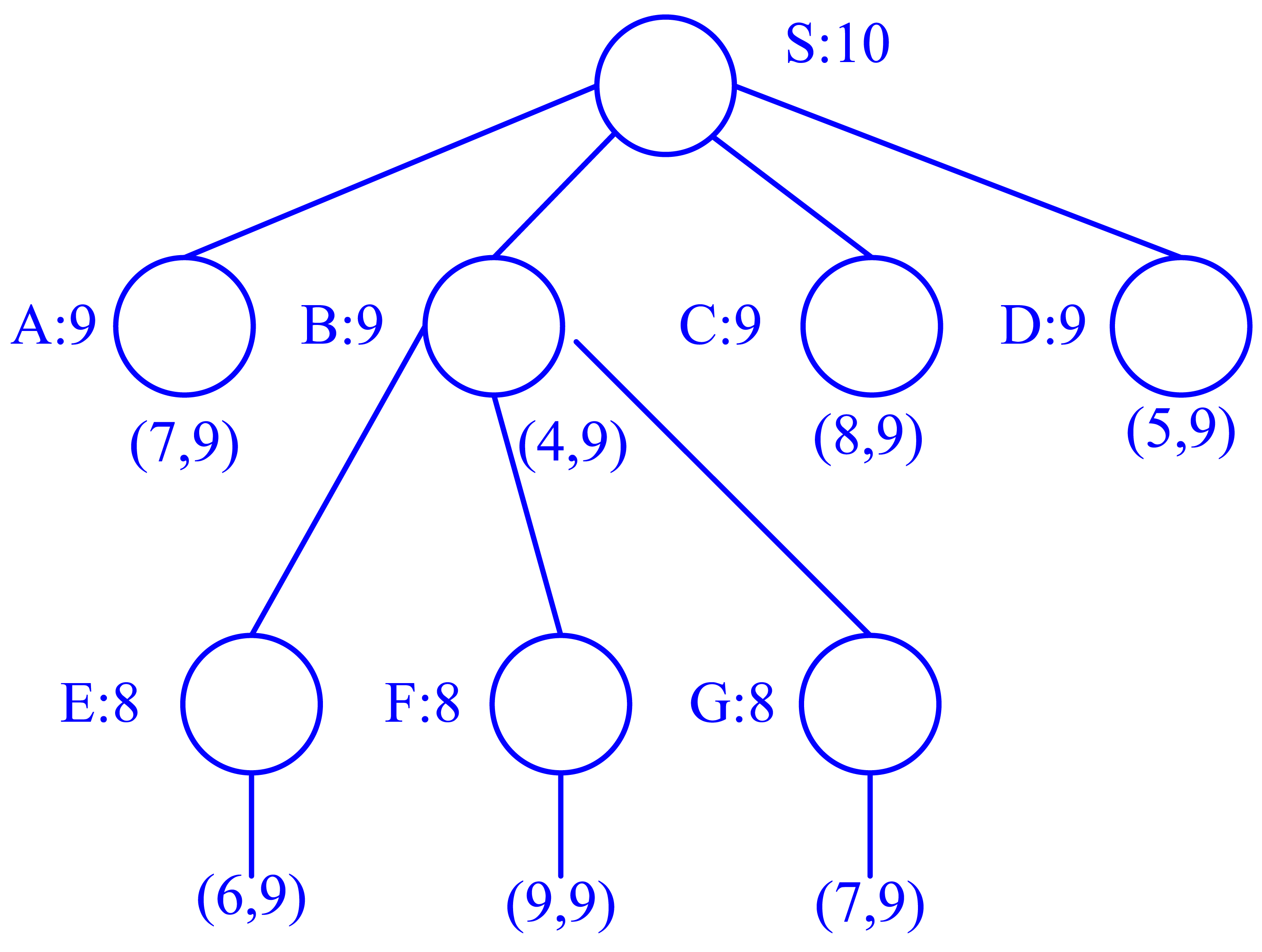
The algorithm of link quality table maintenance and link quality estimation based routing is described in Table 2 and Table 3. We take the example in Figure 1 to illustrate the LQER. Suppose minimum hop field has been established and the minimum hop count of node S is 10. Its forwarding node set includes A, B, C and D with the same hop count 9. The forwarding node set of node B includes E, F and G with hop counts 8. When node S has data packet to send to the sink, it first chooses the node from its forwarding set, the one with the largest value of
, which means the best link quality in history. Not like MHFR, the forwarding node is selected randomly from forwarding set. In this example, node B has the largest value of
and is chosen to forward the packet. The same way is adopted by node B to choose its forwarding nodes. Obviously, node F is the victor. In this way, all the data packets can be forwarded through the shortest and most effectively reliable path and will not generate any extra information. When a node is forwarding the data, all the neighbors with 1 hop less can hear the message. But only the node designated in the message will forward the data. Thus the number of nodes participating in data forwarding is the least and the energy consumption is optimized.
4. Simulation and Evaluation
To evaluate the performance of these routing protocols, we develop a simulation environment named WSNSim, which is based on the energy model of Mote platform and the operation of each node can be defined. We perform the simulation in WSNSim and compare the average energy consumption and packet success rate of MHFR, LQER and MCR. The scalability of LQER is also evaluated. The simulation environment is introduced simply in the subsection and followed by simulation results.
4.1. Simulation Environment: WSNSim
WSNSim developed by Lin et al is a component based, event driven runtime and mote power modeling simulation environment to simulate the energy usage in each node for certain applications [22][23]. The components in WSNSim are similar to Mote developed by University of California at Berkeley, which include CLOCK, SENSOR, ADC, LED, RADIO and APPLICATION. The function of each component is defined as follows.
- -CLOCK:
- in charge of timing, can offer the current simulating time, is the basic of the simulating events.
- -SENSOR:
- provides the sensor data according to the requirement in the application.
- -ADC:
- collects the SENSOR data.
- -LED:
- shows the status of the node.
- -RADIO:
- communicates with other nodes and base station.
- -APPLICATION:
- performs specific application.
The power model used in WSNSim is from Mote MICA2 node with sensor board in a 3V power supply. Table 1 presents the power model for the Mica2 hardware platform. As the table shows, the different CPU power modes cover a wide range of current level, from 103μA in the power-down state up to 8mA when actively executing instructions. Likewise, the choice of radio transmission power affects current consumption considerably, from 3.7mA at -20dB to 21.5mA at +10dBm. However, in many of our applications the radio is almost always listening for incoming messages, which consumes 8mA regardless of transmission activity.
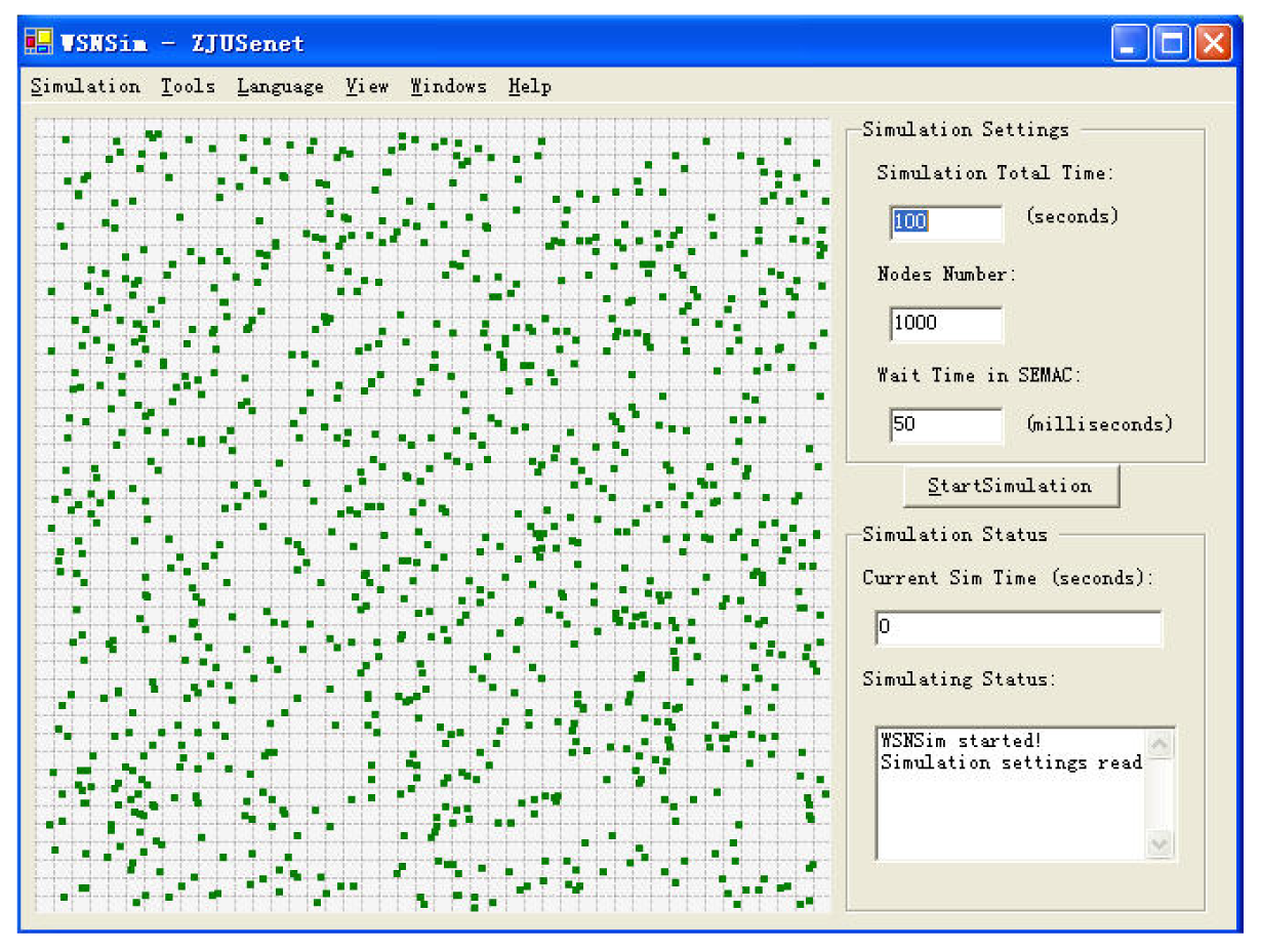
In our simulation, it is assumed that, the power supply for each mote is a constant 3V; when the node is sending messages, the CPU is in the Active state, LED lights up and radio transmission power is averagely at +4dBm thus it consumes 12mA; when the node is listening for messages, the CPU is in the Active state; when the node is receiving messages, the CPU is in the Active state and the radio current is 8mA. When a node goes into sleep, the CPU is in standby state. The initial energy of each node is set to be the same. When the power assumption of one node exceeds the limit, the node is supposed to be disabled. To simplify the model for simulation, we do not consider the CPU cycle power consumption and consider the battery model a linear one. There are two main simulating parameters to be set, that is, the nodes number, N, and the simulating time, T. When the simulating starts, the nodes are randomly deployed in a square with density of 100 nodes per km2 shown in Figure 2 and WSNSim will generate the sensor data in some random distribution according to different applications. The clock is timing, when a timer is fired, an event will occur and WSNSim will check the task queue to perform related operation. The power consumption is calculated and stored for each operation in each node. When the simulation finishes, the energy used in each node will be recorded into files for further analysis.
4.2. Performance Evaluation
In our simulation, Bernoulli loss process model is used to simulate link characteristics [20]. Each node periodically transmits packet to the sink. If the sink does not receive any data, it launches a requirement for retransmission. The node number N is set from 100 to 1000 for different window k. Performance metric of energy efficiency and packet success rate are collected.
4.2.1. Energy Efficiency
There t is the left work time of node i, so the average residual energy of WSNs Ē can be obtained from Equation 2.
For different routing protocols, lager Ē means more energy efficiency after WSNs experience same time under the same conditions.
Figure 3 shows the comparison of average energy consumption over 10000 seconds, where node number N=100, k=9. As a result, it is obvious that LQER can save more energy than MHFR and MCR, especially with time passed. This is because it is not enough to consider only cost and hop count in case the link quality is poor. If the poor link is chosen to deliver the data, loss rate will be high and retransmission will cause extra energy consumption, at the cost of lifetime of WSNs.
4.2.2. Scalability
The number of sensor nodes deployed in studying a phenomenon may be up to thousands or more. For some special application, the number may reach an extreme value of millions. The new routing algorithms must be able to work with such number of nodes. So it is very important and necessary to test the scalability of protocols for a larger scale of WSNs.
Figure 4 shows the difference of average energy consumption of MHFR and LQER over time with k=9, node number from 0 to 1000. As the node number increases, the difference value between MHFR and LQER also increases, which indicates that LQER has a good scalability of energy efficiency. Results are similar in Figure 5, which shows the difference value of average energy consumption of MCR and LQER.
4.2.3. Data Delivery Efficiency
The success rate is the ratio of number of successfully received data packets at a sink to the total number of data packets generated by a source. This metric shows how effective the data delivery is. Also, it is one of most important parameters of QoS. In some applications such as target tracking, data delivery efficiency outweighs energy efficiency. Unless enough reliable data is transmitted to the base station, the target can not be well tracked and controlled.
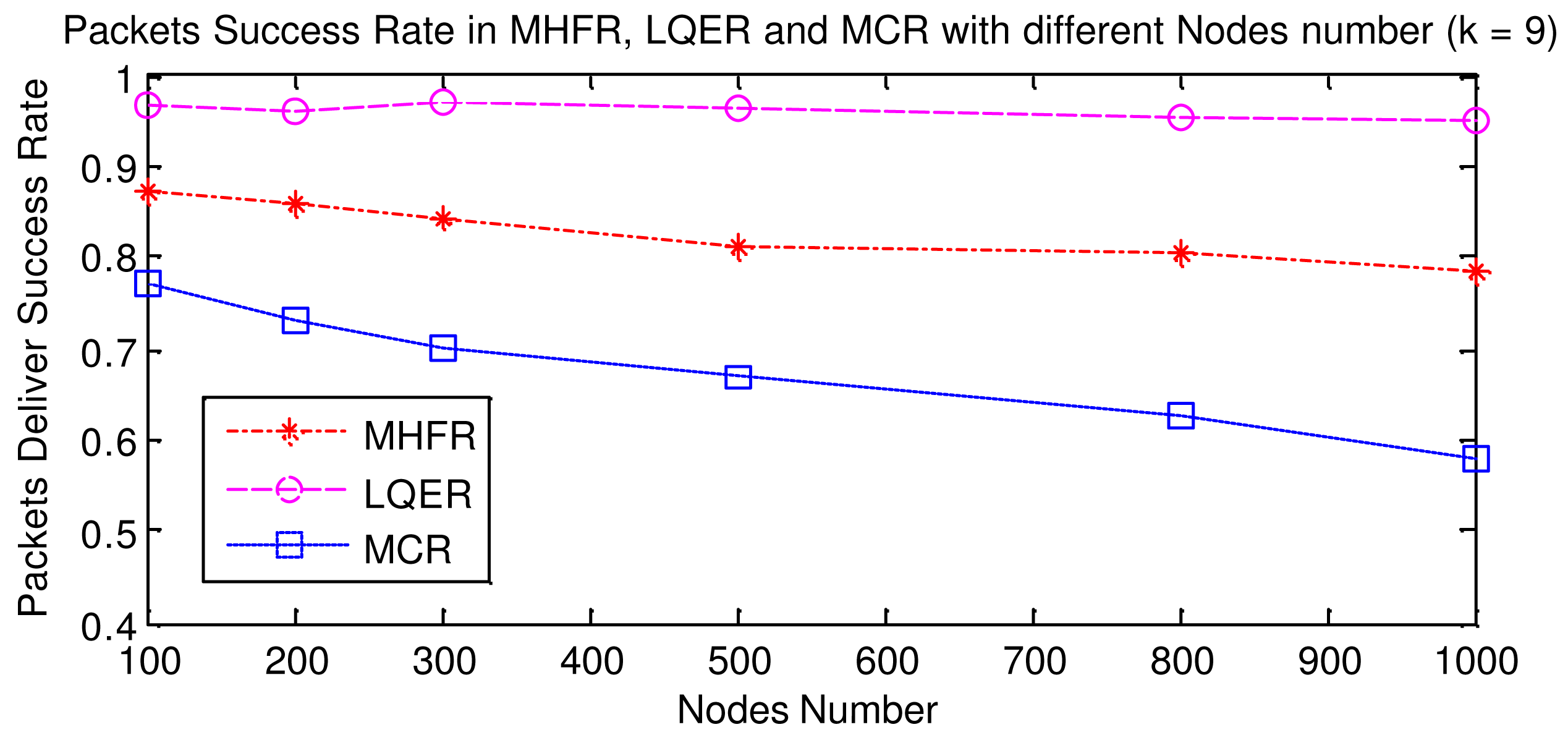
Figure 6 shows the comparison of success rate in LQER, MHFR and MCR with different node number, where k equals to 9. It is clear that the success rate in LQER is higher than that in MHFR and MCR, and when node number increases, the variation is small, which indicates a good scalability of data delivery efficiency. The success rate of MHFR and MCR decline as the node number increases and that of MCR declines more quickly. Particularly, when number of nodes equals to 1000, LQER (95.01%) results in percent of success rate that are more than 21.23% higher than those in MHFR (78.37%), and 86.99% higher than those in MCR (50.81%)
4.2.4. Impact of Window K
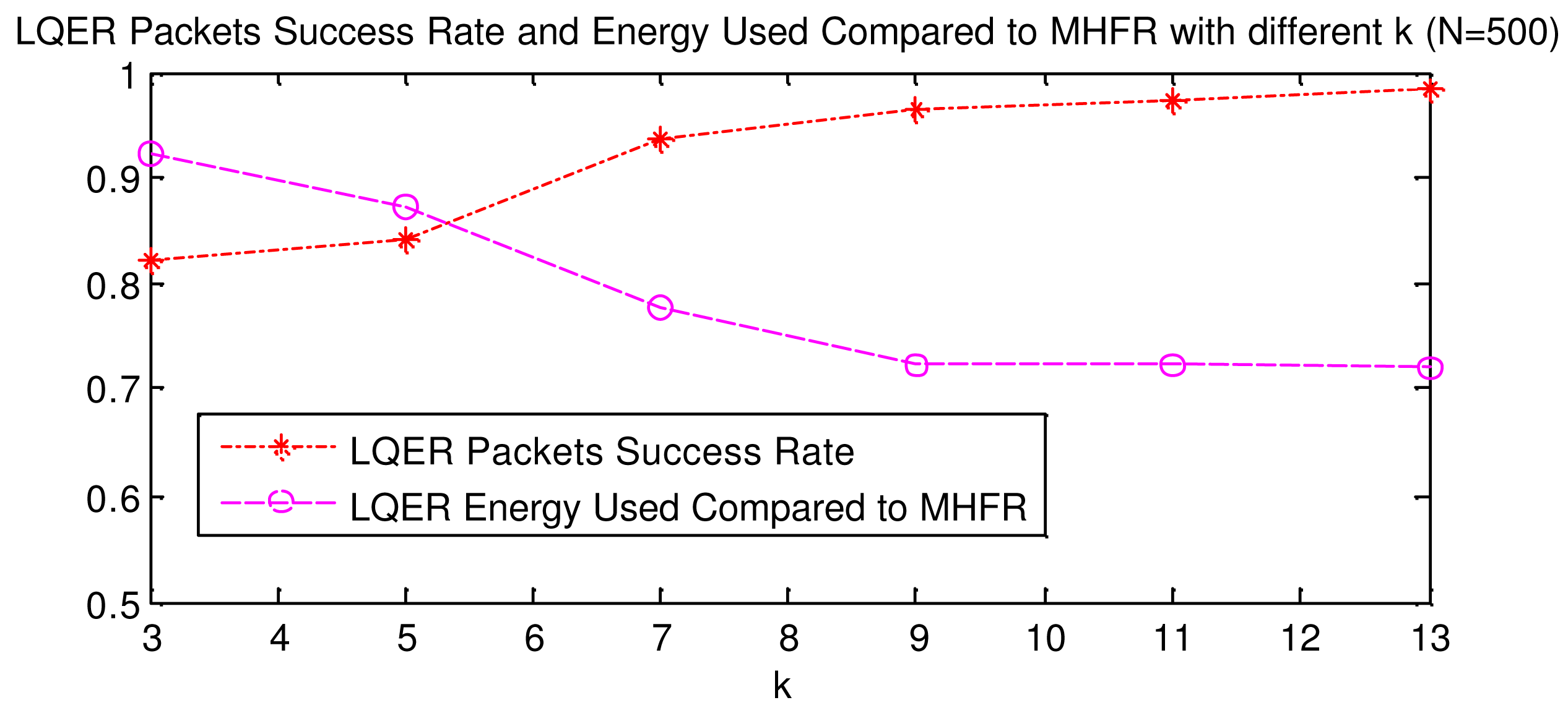
The simulation experiments above have been done with k equal to 9. However, as the value of k reflects how much attention is paid to the historical link quality, different values of k result in different simulation result. Figure 7 shows the success rate of LQER and energy consumption of LQER compared to MHFR with the values of k from 3 to 13, where the node number is 500. It is not that the larger k is, the better the protocol performs. If k is too large, it requires for more storage. From Figure 7, we can see that success rate keeps increasing while k is no larger than 9. After 9, the increase is not so obvious and seems stable. Similar is the energy consumption. It tends not to decline when k is larger than 9. Thus k=9 may be a best choice for link quality estimation.
5. Conclusion
Routing in WSNs has attracted a lot of research attention in last few year. In this paper, the main original contributions includes following parts:
- Propose LQER protocol including hop count field establishment, link table maintenance, link quality estimation with (m, k).
- Show that LQER protocol with proper k can save more energy, have higher success rate and better scalability than MHFR and MCR by simulating in the WSNSim, an environment developed for a large scale of WSNs simulation.
- Find the best k for link quality estimation.
The improvement of energy efficiency is made with a very low computing cost or complexity. Consider of loss rate can meet some special application needs. Furthermore, other performance metrics such as end-to-end delay are to be studied and a real network rather than simulation should be established to further evaluate our routing protocol.
Acknowledgments
This work is supported by Joint Funds of NSFC-Guangdong under grants U0735003; Natural Science Foundation of China under grants No.60604029, 60702081; Natural Science Foundation of Zhejiang Province under grants No.Y106384; the Science and Technology Project of Zhejiang Province under grants No.2007C31038 and the Scientific Research Fund of Zhejiang Provincial Education Department under grants No.20061345.
References
- Ma, Z.; Sun, Y. Research on routing protocol of large wireless sensor network. Computer Engineering and Applications (in chinese) 2004, 165–168. [Google Scholar]
- Ye, F.; Chen, A.; Lu, S.; Zhang, L. Scalable solution to minimum cost forwarding in large sensor networks. Proceedings of 10th International Conference on Computer Communications and Networks.
- Wang, X.; Bi, D.; Ding, L.; Wang, S. Agent collaborative target localization and classification in wireless sensor networks. Sensors 2007, 7, 1359–1386. [Google Scholar]
- Chen, J.; Li, S.; Sun, Y. Novel deployment schemes for mobile sensor networks. Sensors 2007, 7, 2907–2919. [Google Scholar]
- Chen, J.; Cao, K.; Sun, Y.; Yang, X. a. Continuous drug infusion for diabetes therapy: A closed-loop control system design. EURASIP Journal on Wireless Communications and Networking 2008. to appear. [Google Scholar]
- Akyildiz, I.; Su, W.; Sankarasubramaniam, Y.; Cayirci, E. Wireless sensor networks: A survey. Computer Networks 2002, 38, 393–422. [Google Scholar]
- Du, S.; Shi, Z.; W, Z.; Chen, K. Using interacting multiple model particle filter to track airborne targets hidden in blind doppler. Journal of Zhejiang University-Science A 2007, 8(8), 1277–1282. [Google Scholar]
- Akyildiz, I.; Su, W.; Sankarasubramaniam, Y.; Cayirci, E. A survey on sensor networks. IEEE Communications Magazine 2002, 40(8), 102–116. [Google Scholar]
- Akkaya, K.; Younis, M. A survey on routing protocols for wireless sensor network. Ad Hoc Networks 2005, 3(3), 325–349. [Google Scholar]
- Heinzelman, W.; Kulik, J.; Balakrishnan, H. Adaptive protocols for information dissemination in wireless sensor networks. Proceedings of the 6th Annual ACM International Conference on Mobile Computing and Networking 1999, 174–185. [Google Scholar]
- Intanagonwiwat, C.; Govindan, R.; Estrin, D. Directed diffusion: A scalable and robust communication paradigm for sensor networks. Proceedings of the 6th Annual ACM International Conference on Mobile Computing and Networking.
- Rodoplu, V.; Ming, T. Minimum energy mobile wireless networks. IEEE Journal of Selected Areas in Communications 1999, 17(8), 1333–1344. [Google Scholar]
- Xu, Y.; Heidemann, J.; Estrin, D. Geography-informed energy conservation for ad hoc routing. Proceedings of the 7th Annual ACM/IEEE International Conference on Mobile Computing and Networking.
- Yu, Y.; Estrin, D.; Govindan, R. Geographical and energy aware routing: A recursive data dissemination protocol for wireless sensor networks. In Technical Report UCLA-CSD TR-01-0023, UCLA; Computer Science Department, May 2001. [Google Scholar]
- Heinzelman, W.; Chandrakasan, A.; Balakrishnan, H. Energy-efficient communication protocol for wireless sensor networks. Proceeding of the Hawaii International Conference System Sciences.
- Stankovic, J.; Abdelzaher, T.; Lu, C.; Sha, L.; Hou, J. Real-time communication and coordination in embedded sensor networks. Proceedings of The IEEE 2003, 91(7), 1002–1022. [Google Scholar]
- Sohrabi, K.; Gao, J.; Ailawadhi, V.; Pottie, G. Protocols for self-organization of a wireless sensor network. IEEE Personal Communications 2000, 7(5), 16–27. [Google Scholar]
- Akkaya, K.; Younis, M. Energy and QoS aware routing in wireless sensor networks. Cluster Computing 2005, 8(2-3), 179–188. [Google Scholar]
- Chu, M.; Haussecher, H.; Zhao, F. Scalable information-driven sensor querying and routing for ad hoc heterogeneous sensor networks. International Journal of High Performance Computing Applications 2002, 393–313. [Google Scholar]
- Woo, A.; Tong, T.; Culler, D. Taming the underlying challenges of reliable multihop routing in sensor networks. Proceedings of the 1st International Conference on Embedded Networked Sensor Systems 2003, 14–27. [Google Scholar]
- Hamdaoui, M.; Ramanathan, P. A dynamic priority assignment technique for streams with (m,k)- firm deadlines. IEEE Transaction on Computers 1995, 44(4), 1443–1451. [Google Scholar]
- Lin, R. Study of Target-Tracking Oriented Wireleess Sensor Networks. PhD thesis, Zhejiang University, 2005. [Google Scholar]
- Chen, J.; Lin, R.; Sun, Y. Development of simulation environment WSNSim for wireless sensor networks. Chinese Journal of Sensors and Actuators 2005, 19(2), 1–6. [Google Scholar]
Figure 1.
Routing Tree Example

Figure 2.
1000-Nodes Random Network

Figure 3.
Average Energy Consumption of MHFR, LRER and MCR
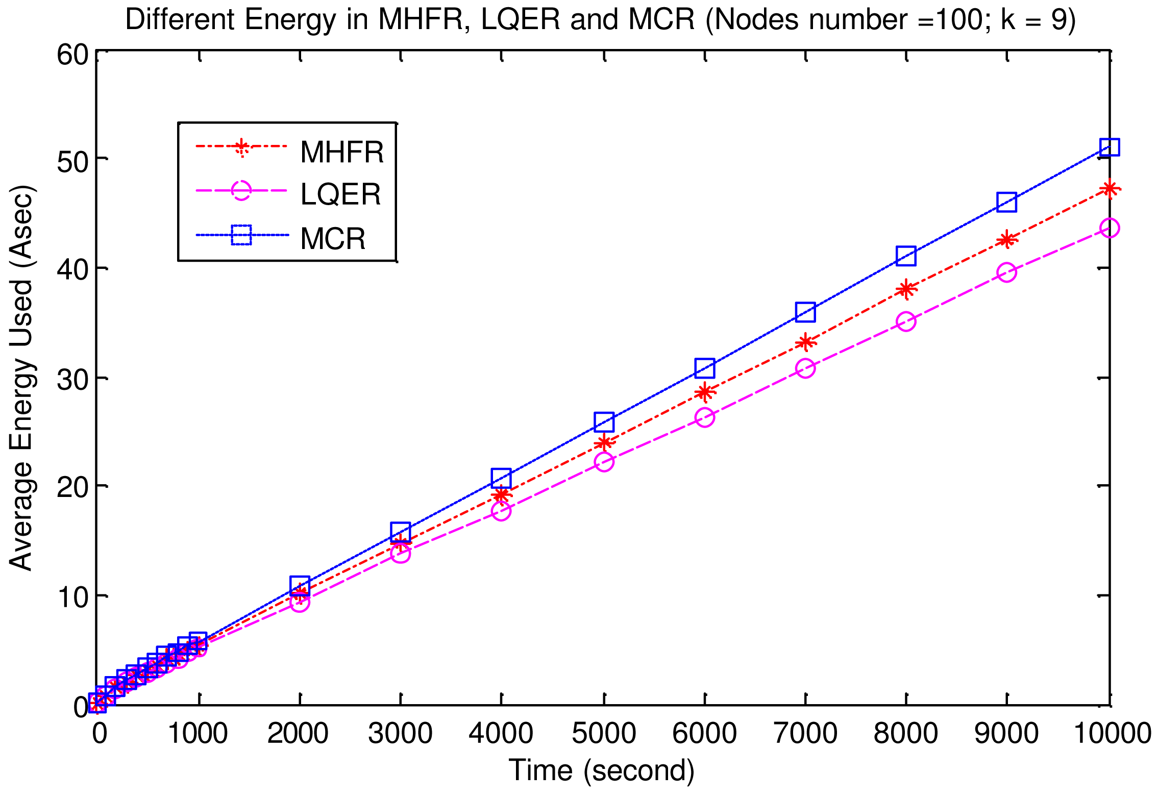
Figure 4.
Difference of Average Energy Consumption in MHFR and LQER
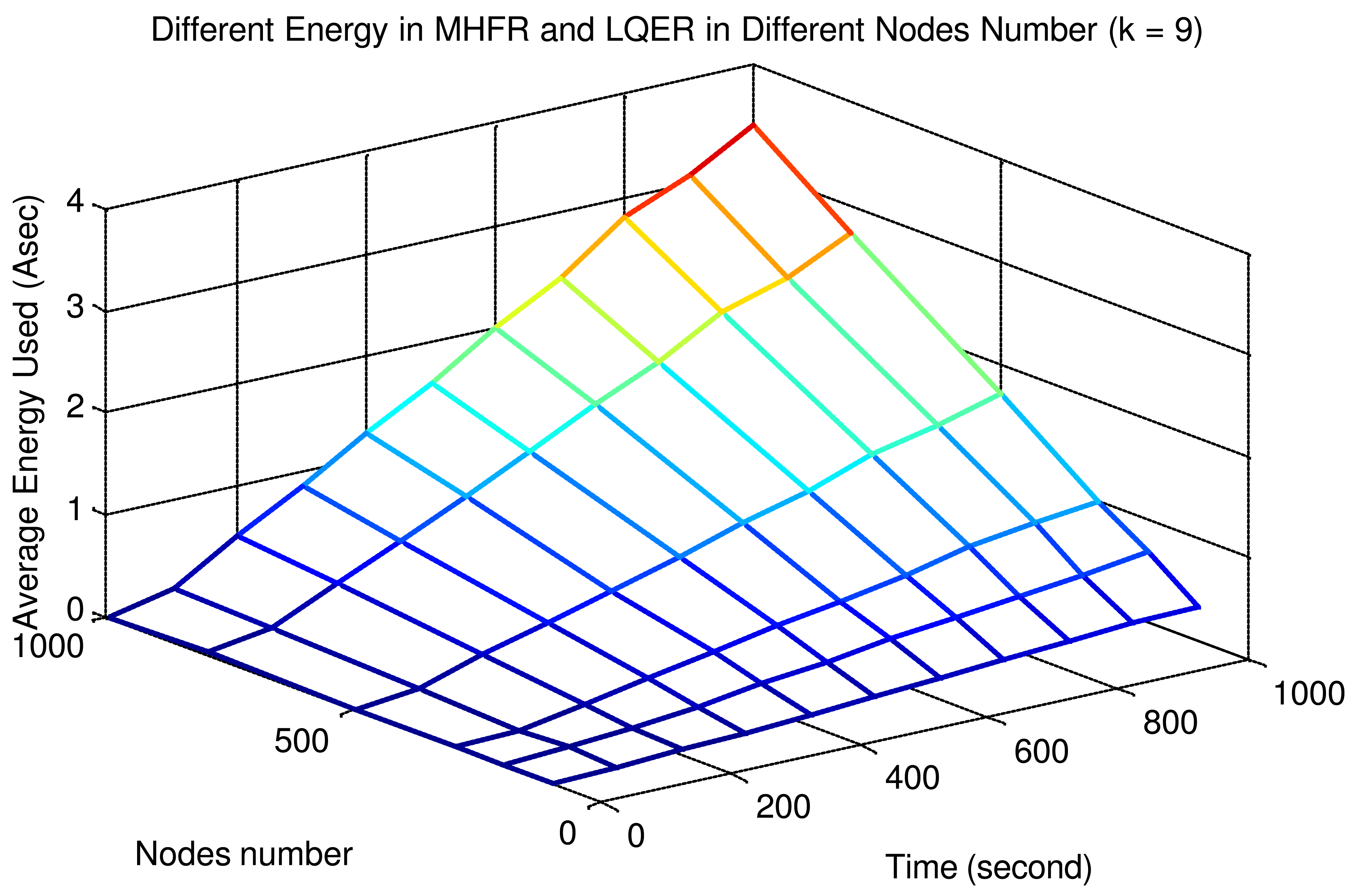
Figure 5.
Difference of Average Energy Consumption in MCR and LQER
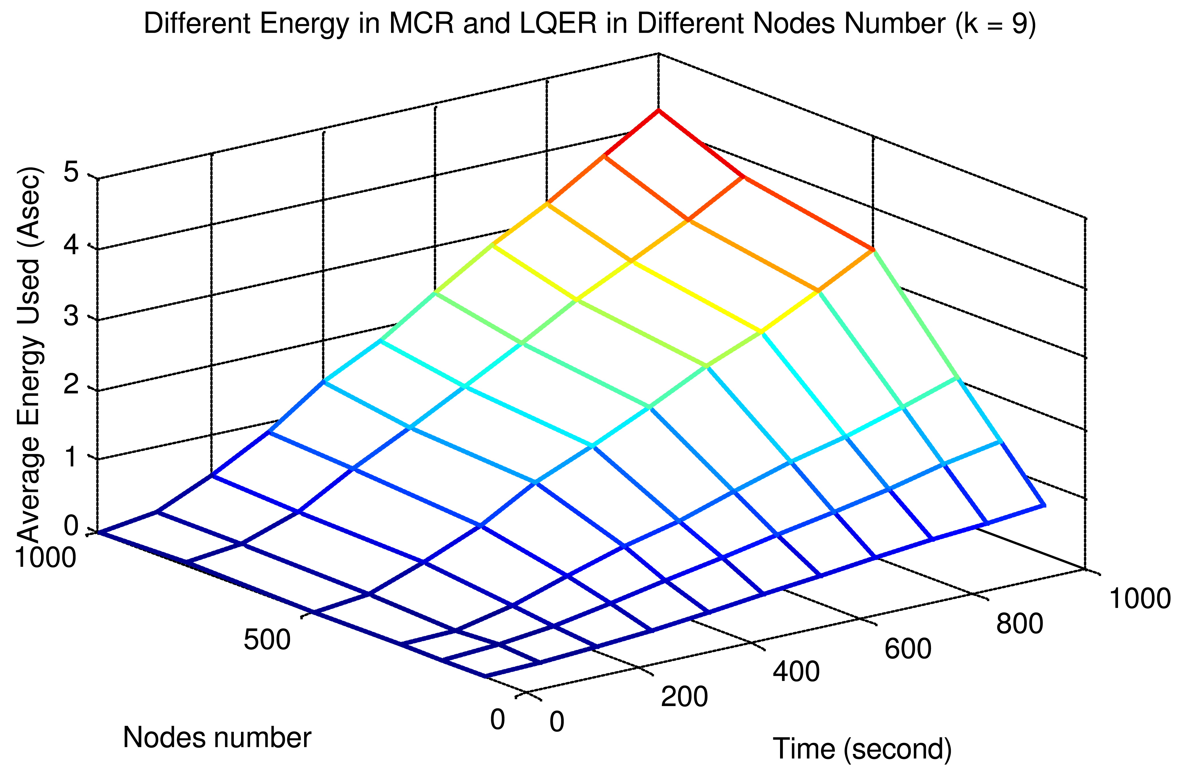
Figure 6.
Success Rate of MHFR, LQER and MCR

Figure 7.
Success Rate of LQER and Energy Consumption of LQER Compared to MHFR

| Mode | Current |
|---|---|
| CPU | |
| Active | 8.0mA |
| Power-down | 103μA |
| ADC Noise Reduce | 1.0mA |
| Standby | 216μA |
| Extended Standby | 223μA |
| LEDS | 2.2mA |
| MICA2 Sensor Board | 0.7mA |
| EEPROM access | |
| Read | 6.2mA |
| Read Time | 565μA |
| Write | 18.4mA |
| Write Time | 12.9μA |
| Radio | |
| Rx | 8mA |
| TX | 12mA |
© 2008 by MDPI Reproduction is permitted for noncommercial purposes.
Share and Cite
MDPI and ACS Style
Chen, J.; Lin, R.; Li, Y.; Sun, Y. LQER: A Link Quality Estimation based Routing for Wireless Sensor Networks. Sensors 2008, 8, 1025-1038. https://doi.org/10.3390/s8021025
AMA Style
Chen J, Lin R, Li Y, Sun Y. LQER: A Link Quality Estimation based Routing for Wireless Sensor Networks. Sensors. 2008; 8(2):1025-1038. https://doi.org/10.3390/s8021025
Chicago/Turabian StyleChen, Jiming, Ruizhong Lin, Yanjun Li, and Youxian Sun. 2008. "LQER: A Link Quality Estimation based Routing for Wireless Sensor Networks" Sensors 8, no. 2: 1025-1038. https://doi.org/10.3390/s8021025