1. Introduction
Linear discrete time system with random state transition and observation matrices arise in many areas such as radar control, missile track estimation, satellite navigation, digital control of chemical processes, economic systems. Koning [
1] gave the Linear Minimum Variance recursive estimation formulae for the linear discrete time dynamic system with random state transit and measurement matrices without detailed rigorous derivation. Such system can be converted to a linear dynamic system with deterministic parameter matrices and state-dependent process and measurement noises. Therefore, the conditions of standard Kalman Filtering are violated and the recursive formulae in [
1] can not be derived directly from the Kalman Filtering Theory. In this paper, a rigorous analysis (mainly in the
appendix) shows that under mild conditions, the converted system still satisfies the conditions of standard Kalman Filtering; therefore, the recursive state estimation of this system is still of the form of a modified Kalman filtering. Reference [
5] shows that this result can be applied to Kalman filtering with uncertain observations, as well as randomly variant dynamic systems with multiple models.
Many advanced systems now make use of large number of sensors in practical applications ranging from aerospace and defense, robotics and automation systems, to the monitoring and control of a process generation plants. An important practical problem in the above systems is to find an optimal state estimator given the observations.
When the processing center can receive all measurements from the local sensors in time, centralized Kalman filtering can be carried out, and the resulting state estimates are optimal in the Mean Square Error (MSE) sense. Unfortunately, due to limited communication bandwidth, or to increase survivability of the system in a poor environment, such as a war situation, every local sensor has to carry on Kalman filtering upon its own observations first for local requirement, and then transmits the processed data-local state estimate to a fusion center. Therefore, the fusion center now needs to fuse all received local estimates to yield a globally optimal state estimate.
Under some regularity conditions, in particular, the assumption of independent sensor noises, an optimal Kalman filtering fusion was proposed in [
11-
12], which was proved to be equivalent to the centralized Kalman filtering using all sensor measurements; therefore, such fusion is globally optimal. Then, Song [
7] proved that under a mild condition the fused state estimate is equivalent to the centralized Kalman filtering using all sensor measurements.
In the multisensor random parameter matrices case, sometimes, even if the original sensor noises are mutually independent, the sensor noises of the converted system are still cross-correlated. Hence, such multisensor system seems not satisfying the conditions for the distributed Kalman filtering fusion given in [
11-
12]. In this paper, it was proved that when the sensor noises or the random measurement matrices of the original system are correlated across sensors, the sensor noises of the converted system are cross-correlated. Even if so, similarly with [
7], centralized random parameter matrices Kalman filtering, where the fusion center can receive all sensor measurements, can still be expressed by a linear combination of the local estimates. Therefore, the performance of the distributed filtering fusion is the same as that of the centralized fusion under the assumption that the expectations of all sensor measurement matrices are of full row rank. Numerical examples are given which support our analysis and show significant performance loss of ignoring the randomness of the parameter matrices.
The remainder of this paper is organized as follows. In Section 2, we present the concept of random parameter matrices Kalman filtering. In Section 3, we present an optimal Kalman filtering fusion with random parameter matrices and show that under a mild condition the fused state estimate is equivalent to the centralized Kalman filtering with all sensor measurements. In Section 4, we show that the result can be applied to Kalman filtering with uncertain observations as well as randomly variant dynamic systems with multiple models. More importantly, we will see that the Kalman filtering with false alarm probability is a special case of Kalman with random parameter matrices. A simulation example is given in Section 5. And finally, in Section 6, we present our conclusions.
2. Random Parameter Matrices Kalman Filtering
Consider a discrete time dynamic system:
where
xk ∈
Rr is the system state,
yk ∈
RN is the measurement matrix,
vk ∈
Rr is the process noise, and
ωk ∈
RN is the measurement noise. The subscript
k is the time index.
Fk ∈
Rr×r and
Hk ∈
RN×r are random matrices.
We assume the system has the following statistical properties: {Fk, Hk, vk, ωk, k = 0,1,2,…} are all sequences of independent random variables temporally and across sequences as well as independent of x0. Moreover, we assume xk and {Fk, Hk, k =0,1,2,…} are mutually independent. The initial statex0, the noises vk, ωkand the parameter matrices Fk, Hk have the following means and covariance.
Where
and
are the (
i,
j)
th entries of matrices
Fk and
Hk, respectively.
Rewriting
Fkand
Hk as:
And substituting
(7),
(8) into
(1),
(2) converts the original system to:
where
System
(9),
(10) has deterministic parameter matrices, but the process noise and observation noise are dependent on the state. Therefore, this would not satisfy the well-known assumptions of the standard Kalman filtering apparently.
In the
appendix, we give a detailed proof that system
(9) and
(10) satisfy all conditions of the standard Kalman filtering and derive the recursive state estimate of the new system as follows:
Theorem 1. The Linear Minimum Variance recursive state estimation of system
(9),
(10) is given by:
where the superscript “+” denotes Moore-Penrose pseudo inverse,
xk+1|k denotes the one-step prediction of
xk+1,
Pk+1|k denotes the covariance of
xk+1|k,
xk+1|k+1 denotes the update of
xk+1 and
Pk+1|k+1 denotes the covariance of
xk+1|k+1.
Compared with the standard Kalman filtering and noting the notations in
(5),
(6), the random parameter matrices Kalman filtering has one more recursion of
as follows:
where
and where
is the (
i,
j)
th entries of
.
3. Random Parameter Matrices Kalman Filtering with Multisensor Fusion
In this section, a new distributed Kalman filtering fusion with random parameter matrices is proposed. The framework of the distributed tracking system is the same as those considered in [
12-
15]. The advantages of transmitting sensor estimates other than sensor measurements can be seen in [
12-
15]. We will show that under a mild condition the fused state estimate is equivalent to the centralized Kalman filtering using all sensor measurements. Therefore, it achieves the best performance.
The
l-sensor dynamic system is given by:
where
xk ∈
Rr is the state,
is the measurement matrix in
i-th sensor,
vk ∈
Rr is the process noise, and
is the measurement noise. Parameter matrices
Fk and
are random. We assume that
,
i,
j =, …
l, is a sequence of independent variables. Every single sensor satisfies the assumption in the last section.
Convert system
(12) to the following one with deterministic parameter matrices:
where
The stacked measurement equation is written as:
where
and the covariance of the noise
ω̃k is given by:
Consider the covariance of the measurement noise of single sensor in new system. By the assumption above, we have:
As shown in the last part of Section 2, every entry of the last matrix term of the above equation is a linear combination of
. Hence, when
and
are correlated, in general,
. Therefore, even if
, i.e., the original sensor noises are mutually independent, the sensor noises of the converted system are still cross-correlated, i.e., R̃k is non-diagonal block matrix.
Luckily, when sensor noises are cross-correlated, in [
7], it was proven that under a mild condition the fuse state estimate is equivalent to the centralized Kalman filtering using all sensor measurments.
According to Theorem 1 and the Kalman filtering formulae given in [
8-
10], the local Kalman filtering at the
i-th sensor is:
where
with covariance of filtering error given by:
or
where
We assume that the system has the following properties: the row dimensions of all sensor measurement matrices
to be less than or equal to the dimension of the state, and all
to be of full row rank. In many practical applications, this assumption is fulfilled very often. Thus, we know
.
According to [
7] and Theorem 1, the centralized Kalman filtering with all sensor data is given by:
where,
is the
i-th column block of
. The covariance of filtering error given by:
or
Where
Using
(15) and
(18), the estimation error covariance of the centralized Kalman filtering is given by using the estimation error covariance of all local filters:
To express the centralized filtering
xk|k in terms of the local filtering, by
(14) and
(15), we have
That is to say that the centralized filtering
(23) and error matrix
(20) are explicitly expressed in terms of the local filtering. Hence, the performance of the distributed random parameter matrices Kalman filtering fusion is the same as that of the centralized random parameter matrices fusion.
4. Applications of Random Parameter Matrices Kalman Filtering
In this section, we will see that the results in the last two sections can be applied to the Kalman filtering with uncertain observations as well as randomly variant dynamic systems with multiple models.
4.1. Application to a General Uncertain Observation
The Kalman filtering with uncertain observation attracted extensive attention [
2-
4]. There are two types of uncertain observations in practice. The first one is that the estimator can exactly know whether the observation fully or partially contains the signal to be estimated, or just contains noise alone (for example, see [
2]). By directly using the optimal estimation theory, the Kalman filter for the first type of uncertain observations can be derived easily. The other uncertain observations belong to the second type, i.e., the estimator cannot know whether the observation fully or partially contains the signal to be estimated or just contains noise alone, but the occurrence probabilities of each case are known. Clearly, the latter is more practical. By applying the random measurement matrix Kalman filtering, we can derive the Kalman filter with the second type of uncertain observations, which is much more general than that in [
2-
4].
Consider a system:
where all the parameter matrices are non-random and a set of multiple observation equations is selected to represent the possible observation case at each time. The random variable
γk is either observable or unobservable. If
γk =
i, the measure matrix is
and the observation noise corresponds to
. When the value of
γk is observable at each time
k, this is an uncertain observation of the first type and the state estimation with measurement
Equation (25) is converted to:
which is obviously the classical Kalman filtering, i.e., the least mean square estimate using the various available observation of
yk. To show the applications of the random measurement matrix Kalman filtering, we focus on the second type of uncertain observation, i.e., in
(25),
γk is unobservable at each time
k, but the probability of occurrence of every available measurement matrix is known.
Consider that in
(25),
γk is unobservable at each time
k, but the probability of the occurrence of each measurement is known. Obviously,
(2) is a more general form of
(25) because only expectation and covariance of
Hk in
(2) are known other than its distribution. The expectation of
Hk can be expressed as:
All that remains in order to apply the random measurement matrix Kalman filtering is just to calculate:
Substituting (
27}) and
(29) into Theorem 1 can immediately obtain the random measurement matrix Kalman filtering of model
(1) and
(25).
In the classical Kalman filtering problem, the observation is always assumed to contain the signal to be estimated. However, in practice, when the exterior interference is strong, i.e., total covariance of the measurement noise is large; the estimator will mistake the noise as the observation sometimes. In radar terminology, this is called a false alarm. Usually, the estimator cannot know whether this happens or not, only the probability of a false alarm is known. In the following, we will show that the Kalman Filtering with a false alarm probability is a special case of the uncertain observations of the above model
(1),
(25) are given.
Consider a discrete dynamic process:
where {
Fk,
hk,
vk,
ωk,
k = 0, 1, 2, …} satisfy the assumptions of standard Kalman filtering.
Fk and
hk are deterministic matrices. The false alarm probability of the observation is 1 –
pk.
Then,we can rewrite the measurement equations as follows:
where the observation matrix
Hk is a binary-valued random with:
In the false alarm case, the state transition matrix is still deterministic, but the measurement matrix is random, by
(35),
(36) and
(37), the covariance of the process and observation noises can be written as follows:
Thus, the Kalman filtering with false alarm probability in this case is given by:
In this section, we consider the application to a general uncertain observation for one sensor case. In a manner analogous to the derivation of Section 4.1, we can also give an application to a general uncertain observation for multisensor case using Section 3. The procedure is omitted here.
4.2. Application to a Multi-Model Dynamic Process
The multiple-model (MM) dynamic process has been considered by many researchers. Although the possible models considered in those papers are quite general and can depend on the state, but no optimal algorithm in the mean square error (MSE) sense was proposed in the past a few decades. On the other hand, when some of the MM systems satisfy the assumptions in this paper, they can be reduced to dynamic models with random transition matrix and thus the optimal real-time filter can be given directly according to the random transition matrix Kalman filtering proposed in Theorem 1.
Consider a system:
where
Fk and
vk are independent sequence, and
Hk is non-random. We use random matrix
Fk to stand for the state transition matrix. The expectation of
Fk can be expressed as:
A necessary step for implementing the random Kalman filtering is to calculate:
Thus, all the recursive formulas of random Kalman filtering can be given by:
5. Numerical Example
In this section, three simulations will be done for a dynamic system with random parameter matrices modeled as an object movement with process noise and measurement noise on the plane. The simulations give the special applications of results in the last section and show that fused random parameter matrices Kalman filtering algorithms can track the object satisfactorily.
Remember that we have rigorously proved in Section 3 that the centralized algorithm using all sensor observations
at the fusion center can be equivalently converted to be distributed algorithm using all sensor estimates
. In addition, the computer simulations we have done show that the simulation results of two algorithms are exactly the same. It turns out that in the following numerical examples, we only compare the distributed random Kalman filtering and the corresponding standard Kalman filtering that ignores the randomness of the parameter matrices. Without loss of generality our examples assume the local sensors send updates each time when they receive a measurement.
Firstly, we consider a three-sensor distributed Kalman filtering fusion problem with false alarm probabilities.
Example 1
The object dynamics and measurement equations are modeled as follows:
where
satisfy the assumptions of standard Kalman filtering. The state transition matrix
Fkis a constant. The measurement matrix is given by:
The false alarm probability of the
l-th sensor is given by:
The initial state
x0 = (50, 0),
. The covariance of the noises are diagonal, given by
Rv =1,
Rωi = 2 ,
i = 1,2,3. Using a Monte-Carlo method of 50 runs, we can evaluate tracking performance of an algorithm by estimating the second moment of the tracking error, given by:
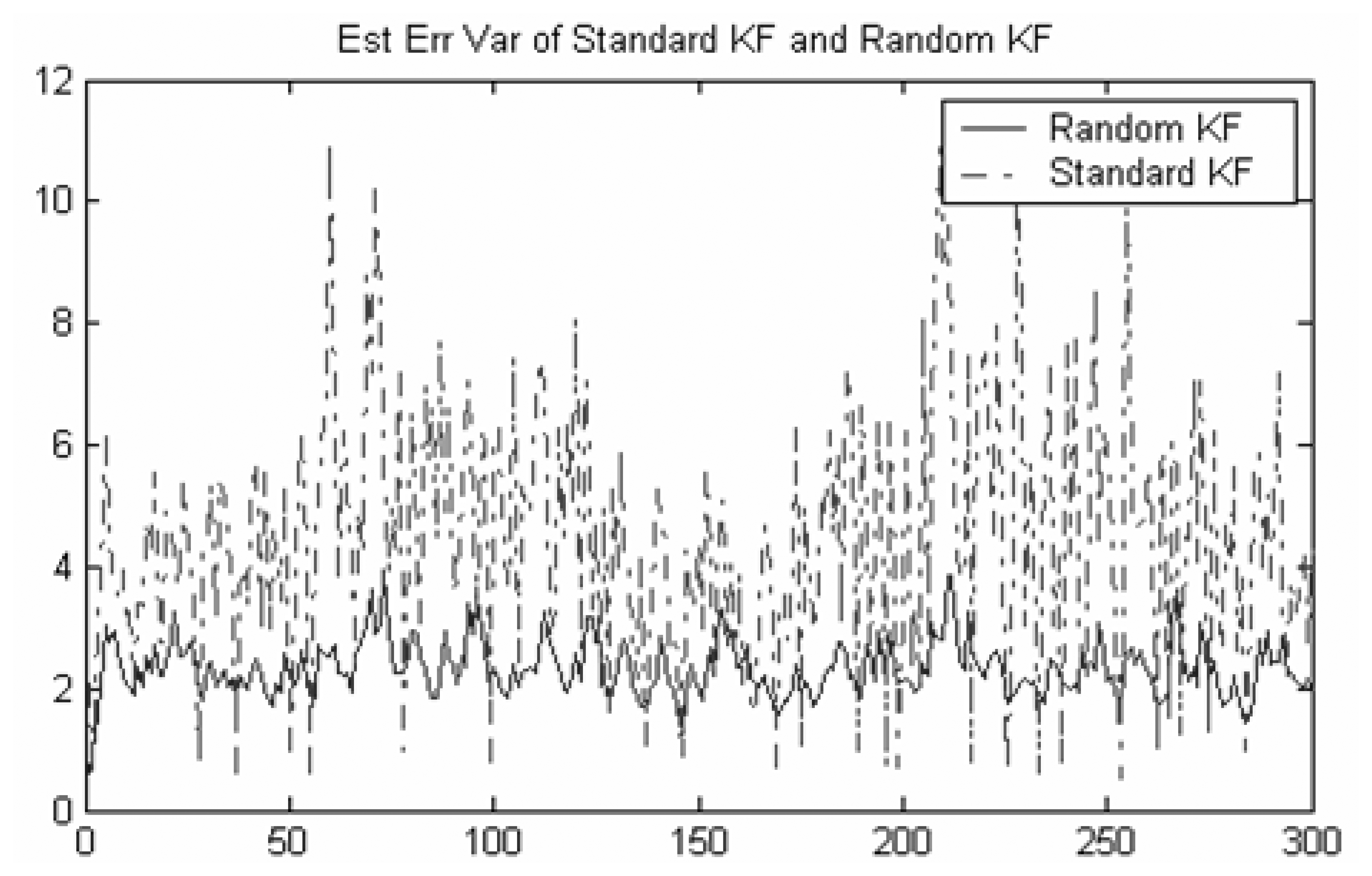
Figure 1 shows that the second moments of tracking error for three sensors Kalman filtering fusion without considering the false alarm (i.e. standard Kalman filtering) and three sensors random Kalman filtering fusion considering the false alarm (i.e. random Kalman filtering), respectively. It can be shown that even if the false alarm probability is very small, the distributed Random Kalman filtering fusion performs much better than the standard Kalman filtering.
In Example 1, both the sensor noises and the random measure matrices of the original system are mutually independent, so the sensor noise of the converted system are mutually independent. Now, we consider another example that both the noises and the random measure matrices of the original system are cross-correlated.
Example 2
The object dynamics and measurement equations are modeled as follows:
where
satisfy the assumptions of standard Kalman filtering. The state transition matrix
Fk and the measurement matrices
are the same as Example 1 and
ωk is a large transition noise. When it happens, the sensors will mistake the transition noise as the observation. The false alarm probability of the transition noise is given by1 −
pk = 0.05. Though the sensor noises
are mutually independent and independent of
ωk, but the total measurement noises
are cross-correlated here. The covariance of the noises are diagonal, given by
Rv = 1,
Rω = 2
Rωi = 0.5,
i = 1,2,3. The initial state
x0 = (50, 0),
.
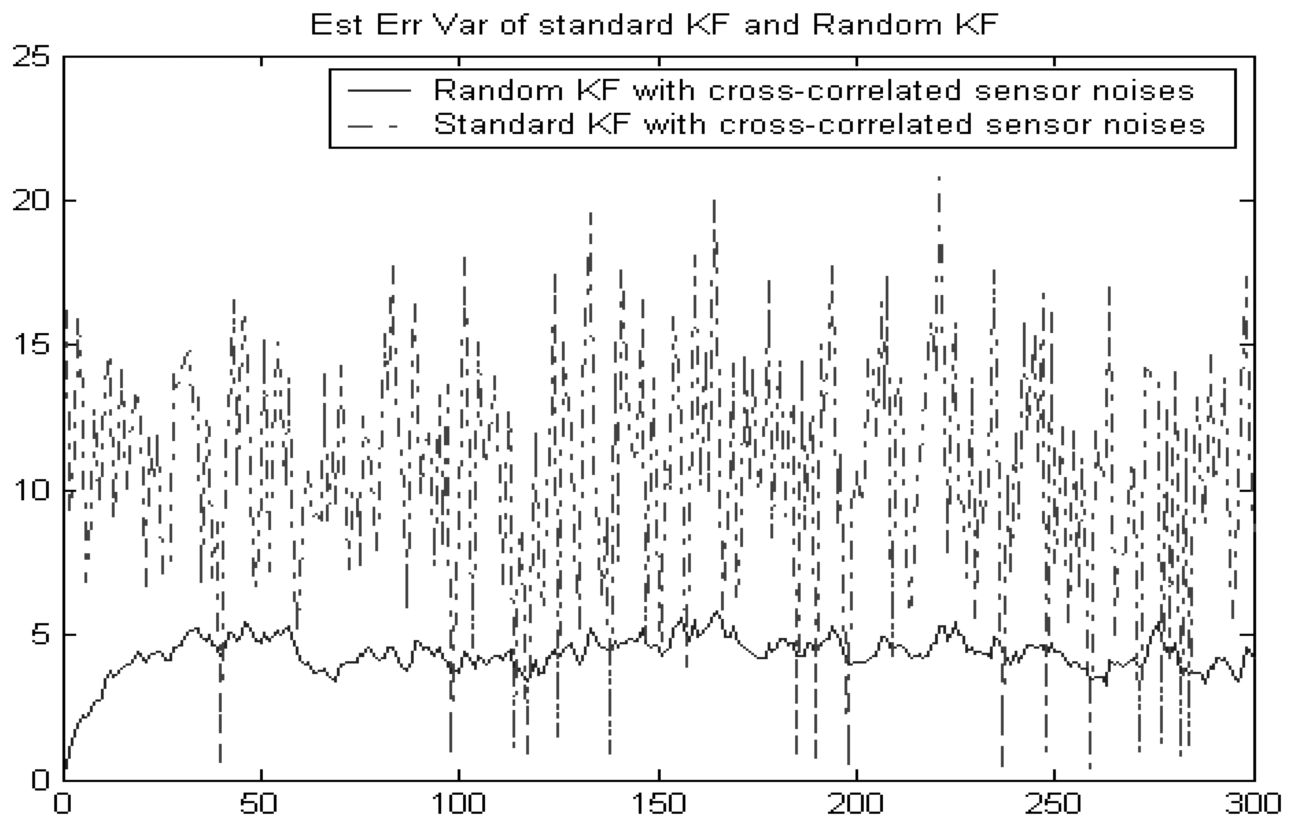
In this example, both the measurement noises and the random measure matrices of the original system are cross-correlated. Hence, the sensor noises of the converted system are cross-correlated.
Figure 2 shows that the random Kalman filtering fusion given in Section 3 still works better than the standard Kalman filtering without considering the false alarm. This implies that the standard Kalman filtering incorrectly assumes that sensor noises are independent.
Example 3
In this simulation, there are three dynamic models with the corresponding probabilities of occurrence available. The object dynamics and measurement matrix in
(40) are given by:
The covariance of the noises are diagonal, given by
Rv = 2,
Rω = 1. In the following, we compare our numerical results with the IMM. Since in this example, the occurrence probability of each model at every time
k is known and mutually independent, it is also the transition probability in the IMM. Therefore, the transition probability matrix ∏ at each time in the IMM is fixed and given by:
Π(
i,
j) here means the transition probability of model
i to model
j . This assumption also implies that the model probability in the IMM is fixed as follows:
Figure 3 shows that the random Kalman filtering given in section 4.2 still works better than the IMM with the fixed transition probability and model probability. This makes sense since the former is optimal in the MSE sense but the latter is not. However, in practice, the occurrence probability of each model is very often dependent on state or observation, and therefore not independent of each other in time. In this case, our new method offers no advantage.
6. Conclusions
In the multisensor random parameter matrices case, it was proven in this paper that when the sensor noises, or the measurement matrices of the original system are correlated across sensors, the sensor noises of the converted system are cross-correlated. Hence, such multisensor system seems not to satisfy the conditions for the standard distributed Kalman filtering fusion. This paper propose a new distributed Kalman filtering fusion with random parameter matrices Kalman filtering and proves that under a mild condition the fused state estimate is equivalent to the centralized Kalman filtering using all sensor measurements, therefore, it achieves the best performance. More importantly, this result can be applied to Kalman filtering with uncertain observations as well as randomly variant dynamic systems with multiple models. The Kalman filtering with false alarm is a special case of Kalman filtering with uncertain observations. Numerical examples are given which support our analysis and show significant performance loss of ignoring the randomness of the parameter matrices.
