Mining the Urban Sprawl Pattern: A Case Study on Sunan, China

Abstract
:
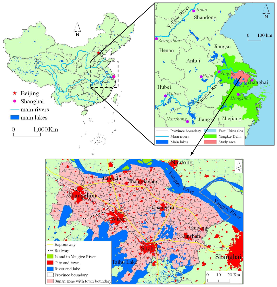
1. Introduction
2. Data
- (a)
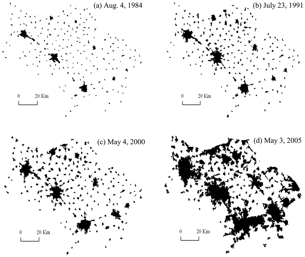
- taking the 1:50,000 scale topographic map from the 1980s as reference, the urban boundaries were digitized based on the 1984 Landsat MSS image (Figure 2a);
- (b)
- taking the boundaries in 1984 as reference, the boundaries in 1991 were digitized based on the Landsat TM image in 1991 (Figure 2b);
- (c)
- taking the boundaries in 1991 as reference, the boundaries in 2000 were drawn out based on the Landsat ETM image in 2000 (Figure 2c);
- (d)
- taking the boundaries in 2000 as reference, the boundaries in 2005 were outlined on the basis of the 23 m spatial resolution IRS-P6 multi-spectral image acquired on May 3, 2005 (Figure 2d).
- (e)
- Finally, for the analysis of fractal dimension, the urban area for each town was exported into a black and white color 4,724 × 4,724 pixel bmp file (each pixel 250 m × 250 m), respectively, representing the urban area and non-urban areas.
3. Methodology
3.1 Fractal dimension
a. Radius method
b. Correlation method
c. Boundary method (or area-perimeter method)
3.2 Compactness index
3.3 Sprawl intensity
3.4 Spatial autocorrelation
a. Global Moran I
b. Global Getis-Ord G
c. Local Moran I
d. Local Getis-Ord G
4. Results
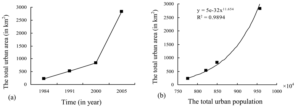
4.1 General situation
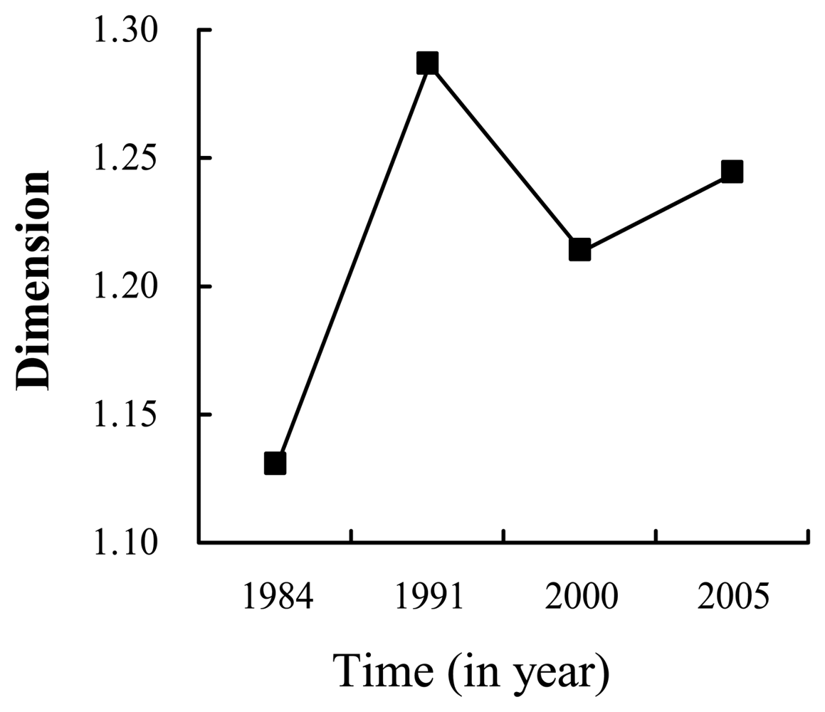
4.2 Homogeneity and compactness
4.3 Sprawl pattern
5. Discussion
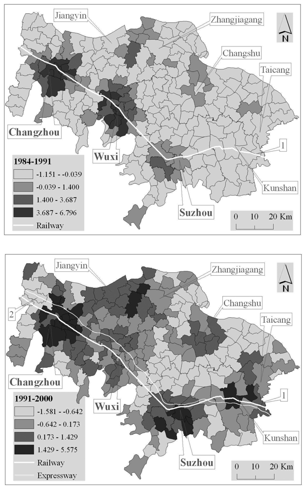
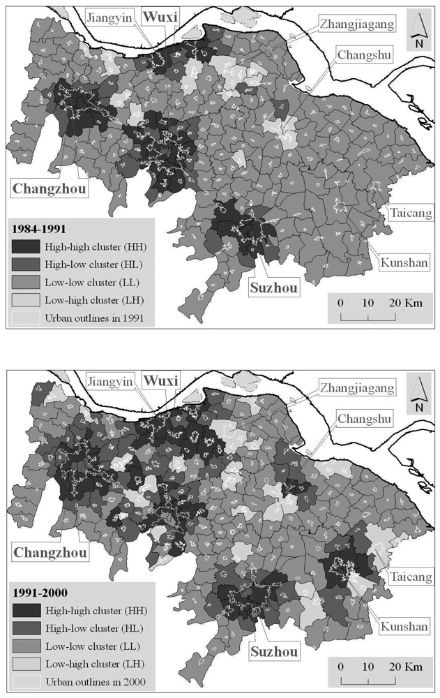
- (a)
- In 1984-1991, there were four hot spots, which were concentrated, respectively, at the four cities, i.e. Changzhou, Wuxi, Suzhou and Jiangyin. The former three are connected directly by the Huning railway (from Nanjing to Shanghai) and the fourth lies along the Yangtze River;
- (b)
- In 1991-2000, the hot spots located at Changzhou and Jiangyin, respectively, still existed but dispersed into a big connected patch; the hot spot located at Suzhou was enlarged and a new one grew up at Kunshan; the one located at Wuxi became weaker;
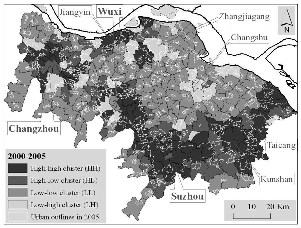
- (c)
- In 2000-2005, the hot spot located at Changzhou still existed, but was becoming weaker and weaker, so did the big connected patch; the one located at Wuxi was enhanced again; noticeably, a zonal hot spot had grown up from Wuxi, through Suzhou, to Kunshan along Huning railway and Huning expressway; additionally, a new one emerged at Taicang along the Yangtze River;
- (d)
- Wholly and generally, the hot spots of urban sprawl were concentric mainly at big cities in the initial stage, where the urban sprawl were self-governed and did not have strong influence on each other; and then, the hot spots gradually spread to their surrounding towns, or they were joined into other hot spots into a big connected patch; with economic and social development, the hot spots spread and dispersed continuously and some were joined into a zonal region along the important transportation axes.
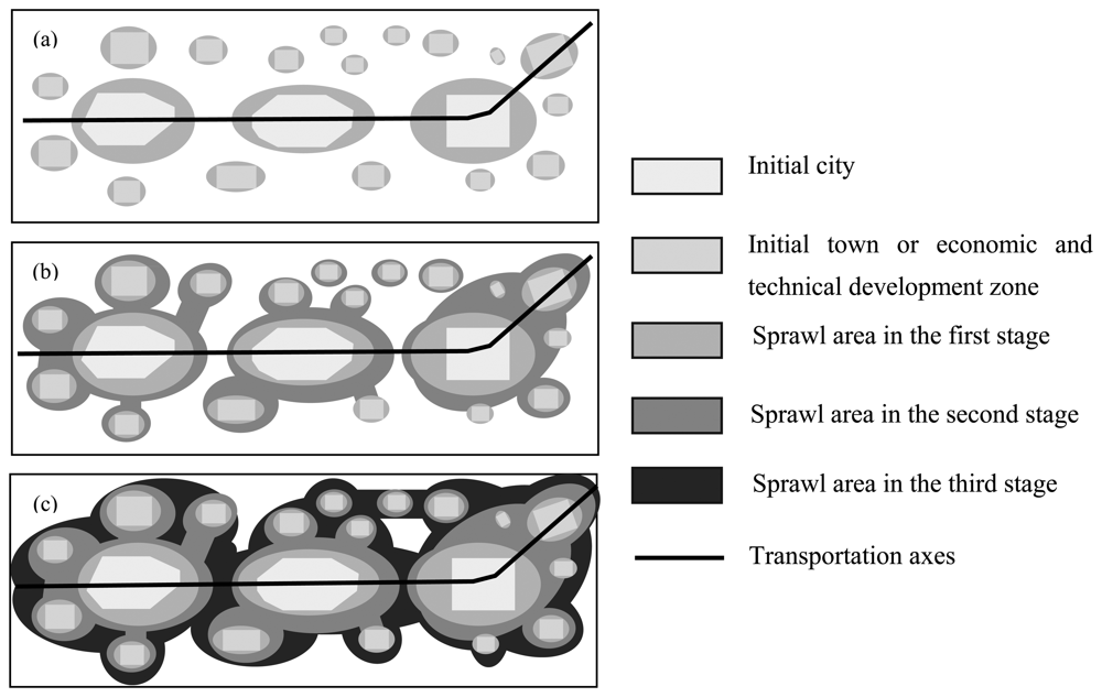
- (a)
- Some big cities benefiting from the preferential policy in the reform and opening-up environment firstly began to grow up at the initial stage, but their sprawls were unconnected to each other (Figure 11);
- (b)
- With the development of economy and the establishment of suitable policies, more and more urban sprawls fused with their surrounding towns, industrial development zones or economic and technical development zones and others; there are more attractions to each other between different cities by more strengthening functions of the important transportation axes or more explicit economic complementarities including city functions (Figure 11b);
- (c)
- The transportation axes are increasingly important in economic development and regional cities are establishing more explicit functional divisions. Gradually, some cities and/or towns were joined together and began to be fused into a big city group or an urban cluster (Figure 11c).
6. Conclusions
Acknowledgments
References and Notes
- Gu, C.; Yu, T.; Chen, J. New characteristics of development of extended metropolitan regions in the time of globalization. Urban Planning 2002, 18, 16–20. (in Chinese). [Google Scholar]
- Tannier, C.; Pumain, D. Fractals in urban geography: a general outline and an empirical example. Cybergeo 2005, 307, 22. [Google Scholar]
- Frankhauser, P. Comparing the morphology of urban patterns in Europe a fractal approach. In European Cities Insights on outskirts, Report COST Action 10 Urban Civil Engineering; Borsdorf, A., Zembri, P., Eds.; Structures: Brussels, 2004; Volume 2, pp. 79–105. [Google Scholar]
- Batty, M.; Longley, P. Fractal Cities: A Geometry of Form and Function; Academic Press: London, 1994; p. 394. [Google Scholar]
- Frankhauser, P. La fractalité des structure urbaines.; Collection Villes, Anthropos: Paris, 1994. [Google Scholar]
- Batty, M.; Kim, S.K. Form follows function: reformulating urban population density functions. Urban Studies 1992, 29, 1043–1070. [Google Scholar]
- Frankhauser, P.; Pumain, D. Fractales et géographie. In Modèles en analyse spatiale; Sanders, L., Ed.; Collection IGAT, Hermes-Lavoisier: Paris, 2001; p. 28. [Google Scholar]
- Longley, P.A.; Mesev, V. Measurement of density gradients and space-filling in urban systems. Pap. Reg. Sci. 2002, 81, 1–28. [Google Scholar]
- Kim, K.S.; Benguigui, L.; Marinov, M. The fractal structure of Seoul's public transportation system. Cities 2003, 20, 31–39. [Google Scholar]
- Portnov, B.A.; Erell, E. Urban clustering: the benefits and drawbacks of location; Ashgate: Aldershot, 2001. [Google Scholar]
- Cliff, A.D.; Ord, J.K. Spatial autocorrelation; Pion: London, 1973. [Google Scholar]
- Ord, J.K.; Getis, A. Local spatial autocorrelation statistics: distributional issue and an application. Geography Analysis 1995, 27, 286–306. [Google Scholar]
- Rey, S.J.; Montouri, B.D. US regional income convergence: a spatial econometric perspective. Reg. Stud. 1999, 33, 143–156. [Google Scholar]
- Matisziw, T.C.; Hipple, J.D. Spatial clustering and state/county legislation: the case of hog production in Missouri. Reg. Stud. 2001, 35, 719–730. [Google Scholar]
- Zhu, C.; Gu, C.; Ma, R.; Zhang, W.; Zhen, F. The influential factors and spatial distribution of floating population in China. ACTA Geogr. Sinica. 2001, 56, 549–560. (in Chinese). [Google Scholar]
- Cohen, J.; Tita, G. Diffusion in homicide: exploring a general method for detecting spatial diffusion processes. J. Quant. Criminol. 1999, 15, 451–493. [Google Scholar]
- Chakravorty, S.; Pelfrey, W.V. Exploratory data analysis of crime patterns: Preliminary findings from the Bronx. In Analyzing Crime Patterns: Frontiers of Practice; Goldsmith, V., Mcguire, P.G., Mollenkopf, J.B., Ross, T.A., Eds.; Sage Publications: Thousand Oaks, CA, 2000; pp. 65–76. [Google Scholar]
- Talen, E. The social equity of urban service distribution: an exploration of park access in Pueblo, Colorado, Macon, Georgia. Urban Geogr. 1997, 18, 521–541. [Google Scholar]
- Gleditsch, K.S.; Ward, M.D. War and peace in space and time: the role of democratization. Int. Stud. Quart. 2000, 44, 1–29. [Google Scholar]
- Schweitzer, F.; Steinbrink, J. Estimation of megacity growth: Simple rules versus complex phenomena. Appl. Geogra. 1998, 18, 69–81. [Google Scholar]
- Carter, H. The study of urban geography; Edward Arnold: Victoria, Australia, 1981. [Google Scholar]
- Ji, W.; Ma, J.; Twibell, R.W.; Underhill, K. Characterizing urban sprawl using multi-stage remote sensing images and landscape metrics. Computers Environment and Urban systems 2006, 30, 861–879. [Google Scholar]
- Mandelbrot, B. The fractal geometry of nature; Freeman: San Francisco, 1977. [Google Scholar]
- De Keersmaeker, M.L.; Frankhauser, P.; Thomas, I. Using Fractal Dimension for characterizing intra-urban diversity. The example of Brussels. Geogr. Anal. 2003, 35, 310–328. [Google Scholar]
- Batty, M.; Xie, Y. Preliminary evidence for a theory of the fractal city. Environment and Planning A. 1996, 28, 1745–1762. [Google Scholar]
- Shen, G. Fractal dimension and fractal growth of urbanized areas. Int. J. Geogr. Inf. Sci. 2002, 16, 419–437. [Google Scholar]
- Frankhauser, P. The fractal approach: a new tool for the spatial analysis of urban agglomerations. Population: An English Selection, special issue New Methodological Approaches in Social Sciences 1998, 205–240. [Google Scholar]
- Johnson, G.D.; Tempelman, A.; Patil, G.P. Fractal based methods in ecology: a review for analysis at multiple spatial scales. Coenoses 1995, 10, 123–131. [Google Scholar]
- Mandelbrot, B. The Fractal Geometry of Nature.; Freeman: San Francisco, 1982. [Google Scholar]
- Li, X.; Yeh, A.G. Analyzing spatial restructuring of land use patterns in a fast growing region using Remote Sensing and GIS. Landscape Urban Plan. 2004, 69, 335–354. [Google Scholar]
- Cliff, A.D.; Ord, J.K. Spatial Processes, Models and Applications; Pion: London, 1981. [Google Scholar]
- Getis, A.; Ord, J.K. The analysis of spatial association by the use of distance statistics. Geogr. Anal. 1992, 24, 189–206. [Google Scholar]
- Anselin, L. Local indicators of spatial association—LISA. Geogr. Anal. 1995, 27, 93–115. [Google Scholar]
- Ma, R.; Pu, Y.; Ma, X. Mining spatial association pattern from GIS database; Science Press of China: Beijing, China, 2007. (in Chinese) [Google Scholar]
- Ord, J.K.; Getis, A. Testing for local spatial autocorrelation in the presence of global autocorrelation. J. Regional Sci. 2001, 41, 411–432. [Google Scholar]
- Ord, J.K.; Getis, A. Distributional Issues Concerning Distance Statistics. Working Paper; The Pennsylvania State University and San Diego State University Presses: Pennsylvania and San Diego, 1994. [Google Scholar]
- Lu, X.; Huang, J.; Sellers, J.M. A global comparative analysis of urban form. 2006. (manuscript).Wong, K.; Shen, J.; Feng, Z.; Gu, C. An Analysis of Dual-Track Urbanization in the Pearl River Delta Since 1980. Tijdschr. Econ. Soc. Ge. 2003, 94, 205–218. [Google Scholar]
- Shen, J. The political economy of dual urbanization in China. The 2nd East Asian Regional Conference in Alternative Geography, Hong Kong; 2000. [Google Scholar]
- Hall, P. Out of control? Urban development in the age of virtualization and globalization. Europaishes Forum Alpbach, Communication and Networks Conference, Alpbach, Tyrol, Austria, August 2002; pp. 15–31. Source: http://www.alpbach.org/deutsch/forum2002/vortraege/hall.pdf (Accessed March 3, 2007).
- Fishman, R. America's New City: Megalopolis Unbound. Wilson Quarterly 1990, 14, 25–45. [Google Scholar]


| Threshold distance = 5,000 m | Threshold distance = 10,000 m | |||||
|---|---|---|---|---|---|---|
| 1984-1991 | 1991-2000 | 2000-2005 | 1984-1991 | 1991-2000 | 2000-2005 | |
| I(d) | 1.620 | 0.200 | 0.456 | 0.707 | 0.167 | 0.222 |
| E(d) | -0.005 | -0.005 | -0.005 | -0.005 | -0.005 | -0.005 |
| Z Score | 15.317 | 1.878 | 4.165 | 18.517 | 4.363 | 5.666 |
| Threshold distance = 5000 m | Threshold distance = 10000 m | |||||
|---|---|---|---|---|---|---|
| 1984-1991 | 1991-2000 | 2000-2005 | 1984-1991 | 1991-2000 | 2000-2005 | |
| G(d) (×10-6) | 9.234 | 2.165 | 1.517 | 19.57 | 7.300 | 5.689 |
| E(d) (×10-6) | 1.034 | 1.034 | 1.034 | 4.454 | 4.454 | 4.454 |
| Z Score | 17.053 | 3.475 | 2.441 | 19.084 | 5.229 | 3.668 |
© 2008 by the authors; licensee Molecular Diversity Preservation International, Basel, Switzerland. This article is an open-access article distributed under the terms and conditions of the Creative Commons Attribution license (http://creativecommons.org/licenses/by/3.0/).
Share and Cite
Ma, R.; Gu, C.; Pu, Y.; Ma, X. Mining the Urban Sprawl Pattern: A Case Study on Sunan, China. Sensors 2008, 8, 6371-6395. https://doi.org/10.3390/s8106371
Ma R, Gu C, Pu Y, Ma X. Mining the Urban Sprawl Pattern: A Case Study on Sunan, China. Sensors. 2008; 8(10):6371-6395. https://doi.org/10.3390/s8106371
Chicago/Turabian StyleMa, Ronghua, Chaolin Gu, Yingxia Pu, and Xiaodong Ma. 2008. "Mining the Urban Sprawl Pattern: A Case Study on Sunan, China" Sensors 8, no. 10: 6371-6395. https://doi.org/10.3390/s8106371
APA StyleMa, R., Gu, C., Pu, Y., & Ma, X. (2008). Mining the Urban Sprawl Pattern: A Case Study on Sunan, China. Sensors, 8(10), 6371-6395. https://doi.org/10.3390/s8106371