Validating Evapotranspiraiton Equations Using Bowen Ratio in New Brunswick, Maritime, Canada

Abstract

Three methods including the Penman-Monteith (PM), Priestley-Taylor (PT), and 1963 Penman equation (PE) for calculating daily reference evapotranspiration (ETo) were evaluated in the Maritime region of Canada with the data collected from 2004 to 2007. An automatically operated meteorological station located on the Potato Research Centre, Agriculture and Agri-Food Canada, Fredericton, New Brunswick, Canada, was used to collect required meteorological data for evapotranspiration modeling. A Bowen Ratio system (BR) was setup near the Environment Canada grade one weather station to provide evapotranspiration observations for the validation research of reference evapotranspiration models. The results showed that the prediction from each of the tested models had a certain degree of offset in comparison with the observations obtained by the BR method. All of the tested models slightly overestimated evapotranspiration compared to the BR system by 5-14%, depending on the method. However, the PM generated a better fit to the pooled dataset while the PT produced the best prediction for the 2007 validation dataset. The PM generated the best estimation of evapotranspiration for year 2004 during a inter-annual comparison. The BR revealed that the average daytime ET for the site was around 2.5 mm day^-1(±0.1) averaged for Julian day 157-276 in 2004 to 2006 and possible condensation was 0.16 mm day^-1 for the same period. Crop coefficient (Kc) varied with different models, for example, 0.42 for the PM, 0.44 for the PT, and 0.67 for the PE with a slight yearly variation. With this set of Kc values, a validation with additional dataset collected in 2007 indicated that all three equations achieved a good fit with observations using the above Kc values. The PT performed slightly better than the other two models. A single factor analysis did not show any statistically significant difference between predicted and measured ET. With a consideration of simplicity and application for scaling up to landscape, this research suggested that the PT is the preferable method for estimating ET values in this region.

1. Introduction

Evapotranspiraiton (ET) is the process by which water is released into the air by evaporation from the soil and transpiration from plant surfaces. Reliably quantifying ET is not only an important task for agriculture managers who deal with water resource management, but also a challenge to scientists working in agriculture and environmental studies, in particular, system modelers, because ET is difficult to directly measure and must be estimated through theoretical modelling. To obtain ET, a reference evapotranspiraiton (ETo) is first estimated through a calibrated ETo model, then the ETo model is modified by a crop coefficient (Kc) to estimate actual ET. Before being applied into a specific region to provide an estimation of ET, ETo models must be calibrated or validated with real ET values obtained by either weighing-lysimeters or other methods such as evaporation pan, eddy covariance, and Bowen ratio (BR).

Lopez-Urrea et al. [1] did a relatively complete comparison among seven evapotranspiration equations for calculating ETo using lysimeter observations in a semiarid climate and concluded that the Penman-Monteith (PM ([2], PM hereafter)) was the most accurate equation among other assessed equations such as Hargreaves [3], FAO-24 Corrected Penman [4;5], and Penman equation (PE, [6]). Several similar studies [7;8] also found that the PM performed well in semiarid climates. On the other hand, other studies found that the PE performed better in humid regions [9] and Priestley-Taylor (PT, [10]) worked better in a nonirrigated pasture site in Florida, USA. While the difference of model configuration may be responsible for the controversial results, the prevailing climate factors could make some models perform better than others for a specific climatic region. Furthermore, the difficulties to obtain real ET values could complicate the comparison and may also be partially responsible for the conflicting reports. Although a report indicated that PM performed better in the Maritime region based on an evaporation pan study [11], a possible comparison of the PM with other ETo models by using measured ET data could provide valuable information with regard to the application and selection of ETo models. Moreover, the PM method has a weakness in predicating ET because it has the highest input demand among other models, which could greatly discourage the application of the model in the real world, particularly, when a scaling-up to landscape is intended.

Up to now, the most standard ET values are considered to be obtained through weighing-lysimeters [2;7;12-15]. However, high cost to set up the system has limited its application and, therefore, the data from lysimeters are not readily available. The Class A pan method is an inexpensive method for measuring potential evapotranspiration. However, the PAN method has some inherited problems and was found to have high uncertainty in validating ETo models [16,11]. Moreover, a further uncertainty will be introduced during derivation of ET from ETo because Kc value must be determined in advance and Kc was found to have daily, seasonal, and regional variations [2]. Very recently, Eddy covariance has been used to estimate ET. However, the expense of this instrumentation has extensively limited its application. Also, there is a lack of comparisons between this method and traditional weighing-lysimeter method. As an alternative, the BR method has been widely used to measure actual ET values, and the collected data can be used for the validation and selection of ETo models [12;14;15;17-19] for a specific region.

There is a concern regarding the accuracy of the BR method, which relates to a particular weather condition or the theory. For example, in semiarid advective environments, the potential errors of the BR method have been found between 5-15% during day time [20;21] and 25-45% in night time [20] compared with the lysimeter method. Todd et. al.'s research [20] indicated that the greatest bias of the BR method occurred on days that were hot, dry, and windy or when the latent heat flux exceeded the available energy.

The uncertainty of the BR method mostly occurs when the Bowen ratio (β = sensible heat (H)/Latent heat (LE)) approaches to -1 because an infinity will be result in the post-processing of raw data. To avoid this, certain number of observations obtained under these conditions must be treated as bad data and discarded during data analysis. In each case, the frequency of the data with this kind of uncertainty could have severe impacts on the estimation of ET and lead to a reduction of the accuracy of the BR method [12;22;23], depending on the prevailing environmental controls in a particular region. Therefore, the interval used to discard the “bad” data could be critical for the proper application of the BR method. A β-value <-0.7 or values in the range -1.3< β<-0.7 were suggested [24-26] to be discarded during post processing of the collected data while a narrower range of -1.25<-0.75 was also proposed [27]. The interval was found to depend on the physical inconsistency of the data and on the resolution limits of the sensor [25] and, in fact, may also be controlled by the prevailing environmental controls in a region. Therefore, determining the suitability of the interval or choosing a proper interval could be an important step in the application of the BR method in estimating ET for a particular region and remains a challenge for the Maritime region of Canada.

There was a comprehensive research on crop coefficient (Kc) variability with different plants and with different development stages of crop by a group of American researchers Allen and Wright ( http://www.kimberly.uidaho.edu/water/asceewri/ _Wright_Kcs_2c.pdfConversion_of). The same group of researchers also recommended that evaluation of crop coefficient values in local climatic condition by local data is necessary because the Kc can vary from region to region or even from field to field because of different micrometeorological conditions. Therefore, Kc derived under local management practice and climatic conditions is essential to the accuracy of the ET estimation. However, there is a lack of such information in the Maritime regions of Canada, which could present certain difficulty to the water management of this region, especially relating to intensive potato production.

The objectives of this study are to: (i) test a proper strategy to apply the Bowen ratio method to estimate valid ET data; (ii) compare the accuracy of ETo models for estimating ET in the Maritime region of Canada; (iii) develop crop coefficients (Kc) for different time and different ETo models used for estimating ET, and (iv) select a most suitable model for estimating ET in the Maritime region of Canada.

2. Material and Methods

2.1. Research site and operating dates

This study was carried out at the weather station (45°55′13.21″ N, 66°36′33.72″ W) of the Potato Research Center (PRC), Agriculture and Agri-Food Canada, Fredericton, New Brunswick, Canada. The station was located in the centre of a grass field which was surrounded by potato fields. The grass field was regularly cut back to 10-15 cm in height. June-September rainfall is around 350 to 450mm, which is approximately 1/3 of annual precipitation in this region. Average soil moisture varied between 0.2 m³m^-3 and 0.303 m³m^-3 with a minimum of 0.12 m³m^-3 and a maximum of 0.39 m³m^-3. Research data were collected during four growing seasons from 2004 to 2007 with a slight difference of start- and end- dates between years, but generally during frost-free periods from late May to early October.

2.2. Bowen Ratio system

A BR system (Campbell Scientific Inc., CSI, hereafter) was deployed to the grass field within the weather station at the beginning of the growing season each year. The system was located in a small grass field encircled by large potato field. The system consisted of a net radiometer Q-7.1 (CSI), a dew-point hygrometer “Dew-10” (General Eastern, MA, USA), two soil heat flux plates (HFT3, CSI), four soil thermocouples (TCAV, CSI), two fine-wire thermocouples (FW05, CSI), and a RM Young wind monitor (CSI). Raw data was averaged and recorded every 20 minutes by a CR21X datalogger (CSI) scanning at an interval of 1 second with simple processing such as for wind correction of net radiation. The processed data was downloaded on a weekly basis and transferred to a desktop computer for storage and further calculations.

2.3. ETo Model descriptions

The following ETo models have been chosen for this research because of their wide acceptance in the estimation of ET in many regions:

2.3.1. FAO-56 Penman-Monteith (PM)

The FAO-56 Penman-Monteith equation is considered as the most precise model to estimate ETo and is expressed as [2]:

$$E{T}_o=\frac{0.408\mathrm{\Delta }(R_n-G)+\gamma \frac{900}{T+273}{U}_2(e_s-e_a)}{\mathrm{\Delta }+\gamma (1+0.34U_2)}$$

(1)

where ET_o is the reference evapotranspiration (mm day^-1); R_n the net radiation measured at 2 m above the crop surface (MJ m^-2 day^-1); G the measured soil heat flux density (MJ m^-2 day^-1) measured by a heat flux plate; T the daily mean air temperature (°C) at 2 m above ground; U₂ the wind speed at 2 m high (m s^-1); e_a the actual vapour pressure (kPa); (e_s-e_a) the saturation vapor pressure deficit at temperature T (kPa); γ the psychrometric constant (0.0677 kPa °C^-1); and e_s the saturation vapour pressure (kPa), estimated as follows [2]:

$$e_s=0.5[e^0(T_{max})+e^0(T_{min})]$$

(2)

where e⁰(T_max) and e⁰(T_min) are the saturated vapor pressure at maximum and minimum temperature, respectively. The actual vapor pressure (e_a) can be calculated as follows when the measurements are missing:

$$e_a=e^0(T_{min})$$

(3)

which assumes that dew point temperature equals minimum temperature in humid regions. The function to calculate saturation vapor pressure at a particular temperature (T) is

$$e^0(T)=0.6108exp[\frac{17.27T}{T+237.3}]$$

(4)

where e⁰ is the vapor pressure (kPa) and T is the mean daily temperature (°C).

Δ in equation 1 is the slope of vapour pressure curve (kPa °C^-1), given by

$$\mathrm{\Delta }=\frac{4098[0.6108exp(\frac{17.27T}{T+237.3})]}{{(T+237.3)}^2}$$

(5)

where T is the mean daily temperature (°C).

2.3.2. Priestley-Taylor (PT)

The Priestley-Taylor [10] equation is expressed as

$$E{T}_o=\frac{\alpha }{\lambda }\frac{\mathrm{\Delta }}{\mathrm{\Delta }+\gamma }(R_n-G)$$

(6)

where ETo, R_n, G, and Δ are as described in equation 1; α a constant (1.26, [10;28;29]); In practice, α was found to vary with different vegetation types, soil moisture conditions, and strength of advection [30;31]; and λ the latent heat of vaporization (2.45 MJ kg^-1).

2.3.3. Penman 1963 (PE)

The Penman equation is expressed as [6]:

$$\mathit{\text{ETo}}=0.8[0.408\frac{\mathrm{\Delta }}{\mathrm{\Delta }+\gamma }Rn+7.5\frac{\gamma }{\gamma +\mathrm{\Delta }}{E}_a]$$

(7)

where Ea is aerodynamic term (mm day^-1), given by

$$Ea=0.35(1+0.00438U_2)(e_s-e_a)$$

(8)

2.4. Bowen Ratio theory (BR)

The BR is an energy-balance method based on forcing its energy closure through the use of H/LE ratio (β) [32;33]. The surface energy budget is expressed as

$$Rn-G_{\mathit{\text{adjust}}}-H-LE=0$$

(9)

where Rn and G_adjust are the measured net radiation and the adjusted soil heat flux (MJ Day^-1). H (MJ Day^-1) is the sensible heat flux; and LE (MJ Day^-1) the latent heat flux, given by:

$$LE=\frac{Rn-G_{\mathit{\text{adjust}}}}{\beta +1}$$

(10)

$$H=\frac{\beta }{1+\beta }(Rn-G_{\mathit{\text{adjust}}})$$

(11)

within a few meters of the surface, H and LE may be expressed as

$$LE=\frac{\rho C_p}{\gamma }Kv\frac{\mathrm{\Delta }e}{\mathrm{\Delta }z}$$

(12)

$$H=-\rho C_p{K}_H\frac{\mathrm{\Delta }T}{\mathrm{\Delta }z}$$

(13)

with assumptions that (i) turbulent transfer coefficients for heat (K_H) and water vapor (Kv) are identical or Kv = K_H[34] and (ii) the two levels at which temperature and humidity are measured must be within the layer of the airflow that has adjusted to that surface so that there is an absence of horizontal gradients of temperature and humidity. β is obtained as

$$\beta \approx \gamma \frac{\partial T/\partial z}{\partial e/\partial z}=\gamma \frac{\mathrm{\Delta }T}{\mathrm{\Delta }e}$$

(14)

where ΔT and Δe are the temperature and vapor pressure difference between the two measurement levels. In practice, when β is close to -1 (e.g. -1.25< β <-0.75), LE and H are assumed to be negligible and are not calculated. Adjusted soil heat flux G_adjust was estimated following Allen et al. [35]:

$$G_{\mathit{\text{adjust}}}=G+0.084\frac{\mathrm{\Delta }{T}_s{Z}_s(C_{s}BD+C_{sw}{W}_s)}{I_t}$$

(15)

where G is the soil heat flux measured by the heat flux plates (MJ day^-1); ΔTs (°C) is the change in soil temperature between the thermocouples, Z_s (0.08m) is the depth of the soil layer being measured; C_s (840 J/kg °C) is the specific heat of dry soil; BD (1200 kg/m³, measured on the site in another study) is the bulk density of soil; C_sw (4190 J/kg °C) is the specific heat capacity of water, W_s (kg H₂O/kg-soil) is the soil water content measurement, mass basis, which was taken from another research carried on the site during same period; and I_t (1200s) is the output interval.

2.5. Data analysis and Statistical processing

The stored data were further processed to produce real ET values (following the formulation in section 2.4 and Bowen Ratio Manual, CSI). The same data set of climate variables (radiation, temperature, relative humidity, and wind speed) collected by the sensors of the BR system was used to derive daily statistics that were used to estimate ETo by models defined in equations 1, 6, and 7. Kc values were calculated for each method using measured ET divided by modelled ETo (Kc = ET/ETo). Data collected during year 2007 were used to validate ETo models with the Kc values derived from the dataset of year 2004 to 2006. Regression analysis and single factor analysis were used to check the performance of each model.

3. Results and Discussion

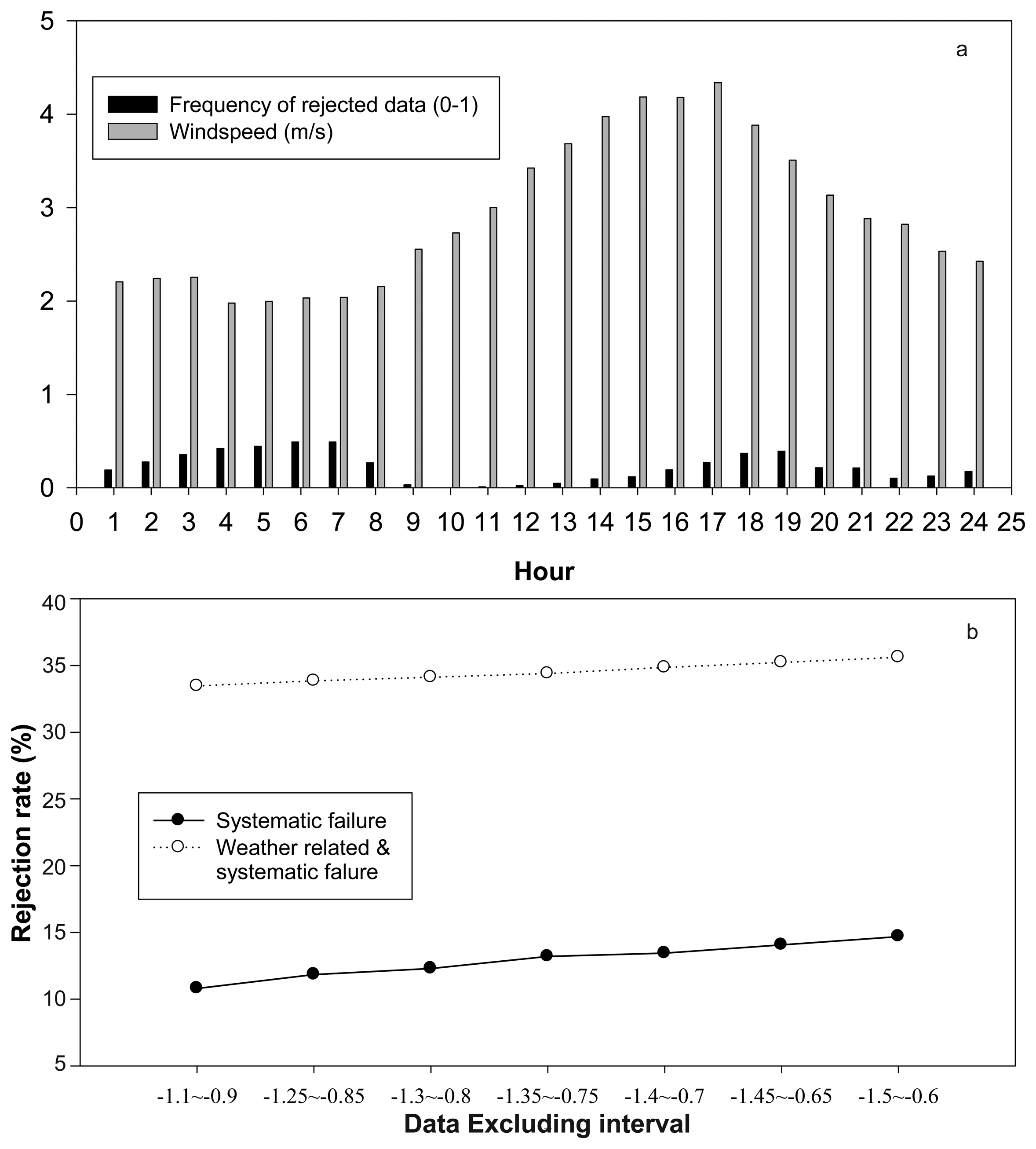
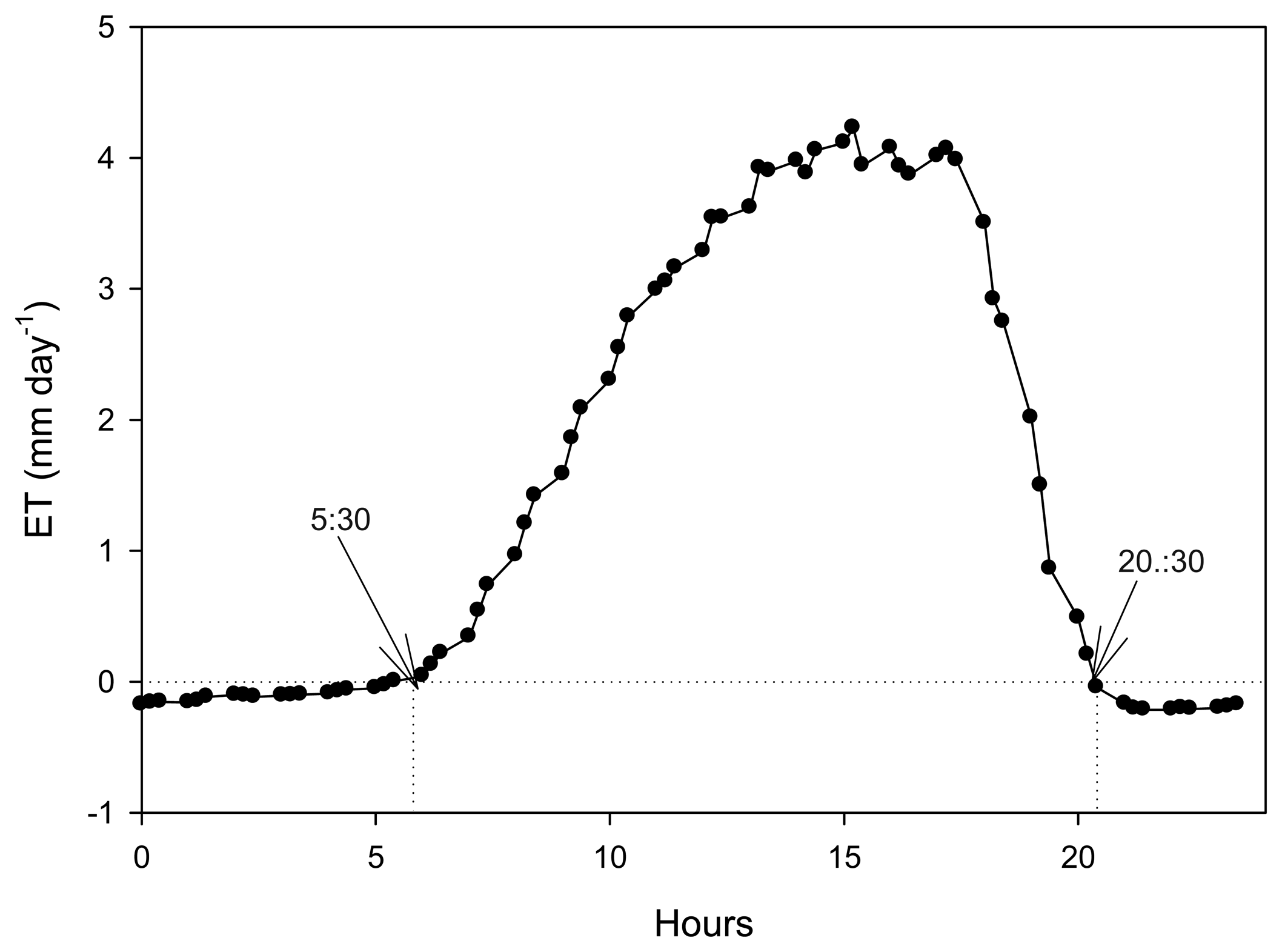
3.1. Bowen ratio method and its performance in the Maritime region

As shown in figure 1a, data quality varied with time of the day. Applying a filter of -1.3 to -0.7 of β, it was found that from the early morning 1:00 to 7:00 AM, the data rejection rate increased gradually from 19% to about 40%, then, dropped down quickly and reached 0 at 9:00 AM. The peak data rejection rate seemed to be related to the early morning quiet period or low wind speed condition of the day. Afterward, a low rejection rate was maintained until 16:00 PM in the afternoon. Starting from this time, a second peak of data rejection rate was started and gradually reached a maximum at 17:00 to 19:00 PM. Then the rejection rate oscillated throughout the night. On a daily basis, the variation of data rejection rate was similar to that reported in other studies, but the average data rejection rate of 20% was different from that of the previous research (38%, [21]). In a similar research, Perez et al. [25] found a total of 40% of the data, which corresponded to the night-time period and to precipitation or irrigation events, were often rejected. They found that, for consistent data and depending on the site, the rejection number could range from 4 to 40%. The results from our research are within the range defined by Perez et al. [25]. The average difference between two rejection rates in our research and in Perez et al.'s research could be attributed to the variability of leading environmental controls at both research sites. Perez et al.'s research [25] was conducted in a region with semi-continental climatic region with annual precipitation below 420 mm while the study site in this research can receive more than 1200 mm of precipitation in a year. In their dry or semiarid climates with very limited soil moisture available, vapor pressure gradients were smaller because the soil and the crop were dry, leading to a larger excluding interval of data [25]. In contrast, our site received more precipitation with a larger vapor pressure gradient, leading to a smaller excluded interval of bad data.

Further analysis of a dataset collected in 2007 indicated that the rejection rate did not change very much with different excluding interval or discarding range (figure 1b). Only a change of <5% was detected from the narrowest to the widest discarding ranges. A further analysis indicated that 50% of the rejection rate was mainly related to the BR theory itself (i.e., when the β→-1) while the rest may be attributed to either noise caused by instrument or other related factors such as rain and evening, during the night, and in the early morning when net radiation and soil heat flux have changed from positive to negative [25]. Although this proportion of the rejection rate between theory-related and other factor related reasons was not fixed and could be changed a little over time and region, it is reasonable to suggest an excluding interval of -1.35∼ -0.75 of β for the BR post data processing in our research region. With this range, about 20% of the data could be excluded as uncertainty during post data processing, leading to a reliable estimation of evapotranspiration.

Although the accuracy may be site- and climate- depended BR method was reported to overestimate ET by 5-15% [21] during day time and 25-45% [20] during night time compared with lysimeter observations. It is possible that the offset may not be linearly related to the weather condition. However, in this research, we did not have lysimeter data to verify the potential bias of the BR method and assumed the BR measurements to be “real” ET values. This is a reasonable assumption for our current study to derive Kc values and compare different models because we focused on the variation pattern instead of absolute values.

Figure 2 shows an averaged diurnal cycle of ET measured by BR method. From 20:30 to 5:30 of the next day, a little condensation occurred, about 3.2% of daily total water exchange. During day time, the ET gradually increased and reached a maximum value, about 3.8 to 4.0 mm day^-1 at 14: 00 and remained around these values until 19:00. After 19:00, the ET quickly dropped down to 0 at about 20:30. On the daily basis, the day-time ET for the period of Julian Day 164-276 (year 2004-2006) averaged 2.5 mm day^-1 and night-time -0.16 mm day^-1.

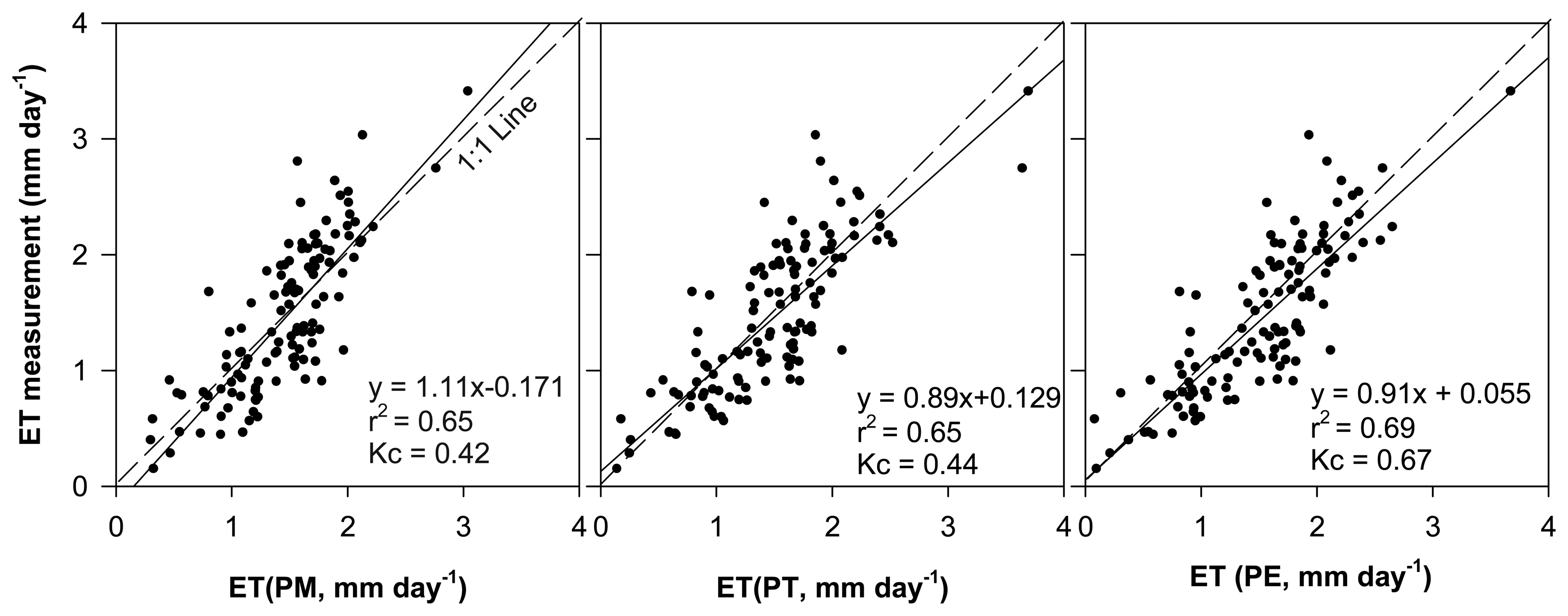
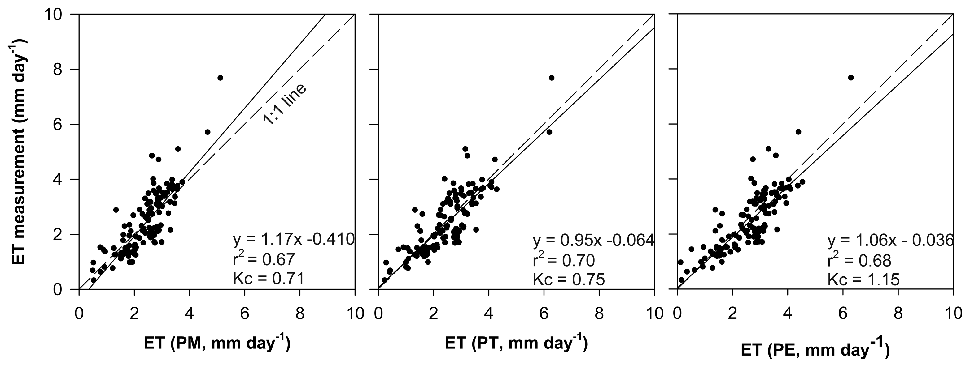
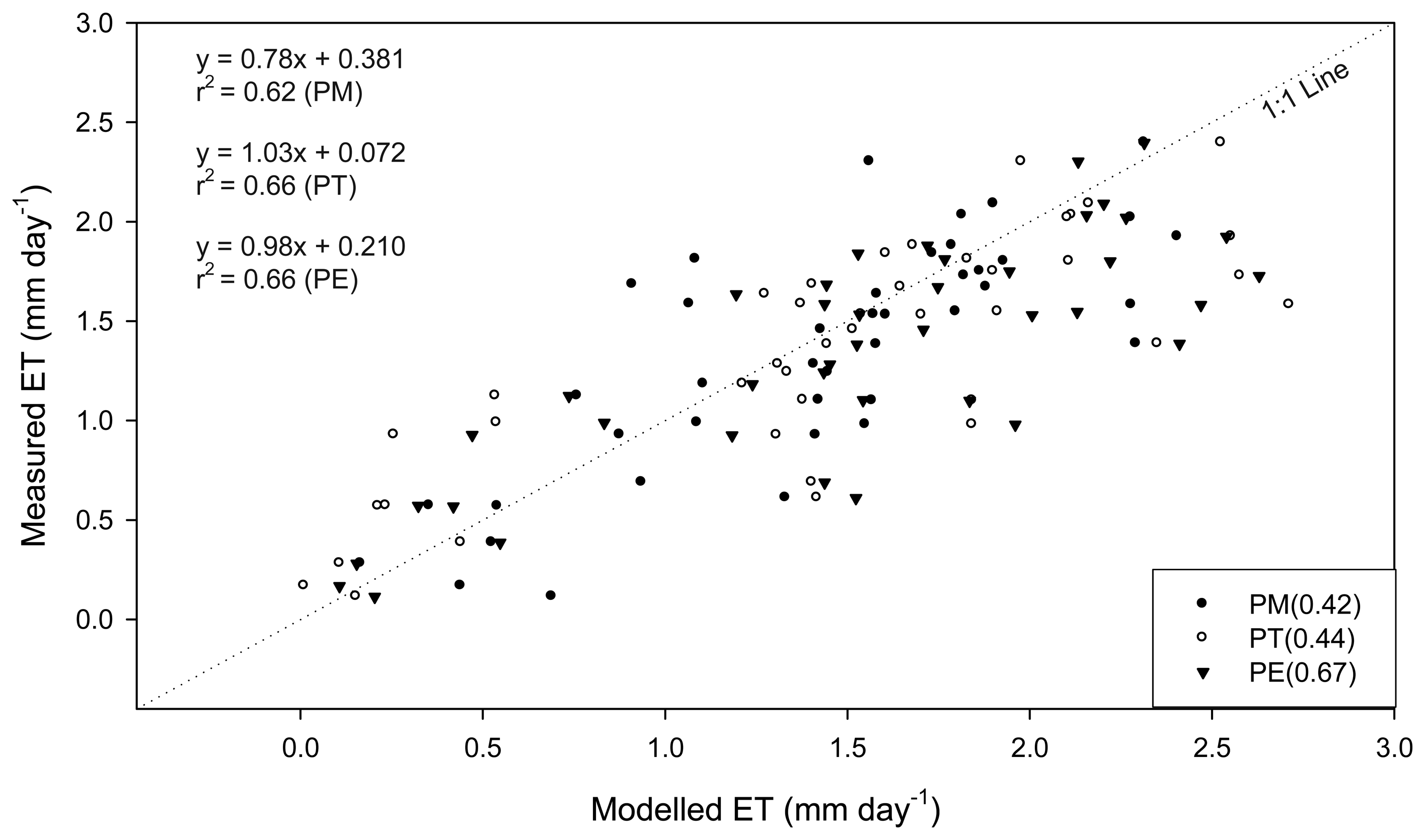
3.2. Comparisons of different ETo methods

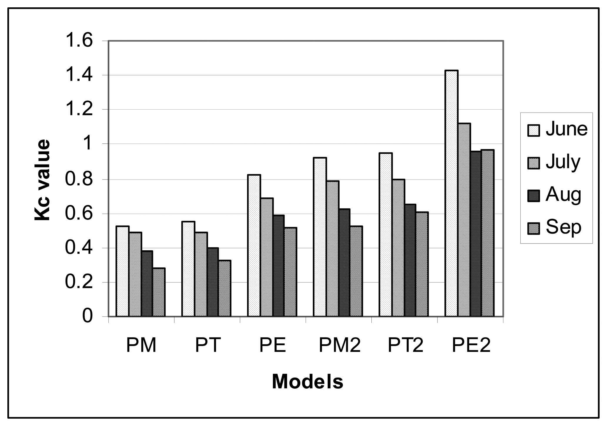
A comparison between ET measurements and predications by different models is showed in Figure 3.

These comparisons were made with different Kc values for different methods with all datasets pooled for different years (2004-2006). Although it can be seen that all models demonstrated a reasonable fit to the observations, and the PE method performed slightly better than the PM and PT, Given the adjustable parameter constant (α) in the PT, it is possible to get a better performance from this method. However, we compared the different methods with original format and investigated the Kc variability. Therefore, we did not change the constants in this comparison. After night-time data were removed, a similar comparison was made. The results are shown in Figure 4. Obviously, the fitting got better except for the PM method. A larger improvement was made to the PT method while improvement to the PE method was minor. A single factor analysis with all data showed that all of the methods applied here did not show significant difference from the measured ET (p>0.3,

Table 1. Single factor analysis of evapotranspiraiton measured by the BR system and calculated with different models (PM, Penman-Monteith; PT, Priestley-Taylor; PE, Penman 1963). A variable Kc value (for different models) has been used in the calculations.

Methods*	Samples	Mean	Variance	P-value**	F***	F crit	Kc*	RE(%)****
PM	318	1.46	0.23	0.92	0.01	/	0.42	0.8
PT	318	1.49	0.35	0.65	0.21	/	0.44	2.5
PE	318	1.53	0.36	0.32	0.97	/	0.67	5.5
ET	318	1.45	0.43			3.88

^*For each method, a corresponding Kc values derived from the data during previous 3 years was applied to the modeled value by different methods. For example, 0.42 was applied to the PM, 0.44 to the PT, and 0.67 to the PE, respectively.

^**A higher P value indicates a insignificant difference between measured ET and modeled ET.

^***F>Fcrit means a significant difference between two variables.

^****RE is relative bias, calculated as (Modelled ETmean-Measured ETmean)/Measured ETmean×100.

).

However, as showed in Table 1, the PM method had the highest p value (0.92) and the least relative bias (0.8%) from measured ET. The PT method performed slightly poorer while the PE had the highest relative bias (5.5%). After removing the night-time data, the PM methods performed even better (

Table 2. Single factor analysis of modeled (PM, Penman-Monteith; PT, Priestley-Taylor; PE, Penman 1963) and measured ET with night-time data removed*

Methods	Samples	Mean	Variance	P-value	F	F crit	Kc	RE(%)
PM	318	2.46	0.64	0.98	0.00	/	0.71	0.0
PT	318	2.53	1.02	0.59	0.29	/	0.75	2.8
PE	318	2.62	1.05	0.24	1.41	/	1.15	6.9
ET		2.46	1.31			3.88

^*see the footnote of Table 1 for the explanation of each letter in the table.

). In comparison, the relative bias of ETo models can be ranked as PM<PT<PE for both night-time included and night-time excluded data (Table 1 and Table 2) with relative error ranged from 0.% to 6.9%. The results suggest that all tested methods can generate a very good mean estimation of ET although locally the bias may be high in some days.

3.3. Kc variability

As shown in Figure 5, Kc values varied with different methods. No matter if the night-time data were included or not, the Kc values showed a daily evolution and varied between 0.3 and 1.4, depending on the method.

After the night-time data were removed during the comparison, the Kc values increased and model performance was improved. Normally, the average Kc increased 69, 71, 72% for the PM, PT, and PM method, respectively. The Kc values also displayed some variability over time. June had the highest Kc values (Figure 5) which was corresponding to the emergence and early growing stage of potato in this research. Kc decreased in July (vegetation growth stage), and further decreased in August (tuber set and bulking stage). In general, potato reaches its medium canopy development during July in this region. The decrease of Kc over different months seemed to be consistent for entire dataset. For night-time removed data, there was less variability of Kc values between August and September. In similar research, Peacock and Hess [19] found that Kc values were inconsistent from day to day but generally less than unity (i.e., 1). The inconsistency was thought to be caused by variations in meteorological conditions such as high radiation, dry canopy, crop type, crop growth stages, and soil evaporation [2]. Precipitation and wind may also be responsible for the Kc difference. In other research, Allen and Wright ( http://www.kimberly.uidaho.edu/water/asceewri/Conversion_of_Wright_Kcs_2c.pdf) reported an extensive list of Kc for various plants, which were based on the 1992 Kimberly Penman method (another version of Penman-Monteith method but using alfalfa as reference plants instead of grass) for temperate climatic region in USA. In their technical note, a 0.2 to 0.7 of Kc value were reported for potatoes. Our research resulted in a 0.2-0.8 of Kc range for the PM-based method, which is similar to Allen and Wright's results. However, it is possible that different management activity and weather conditions around the time period could create some difference in Kc values.

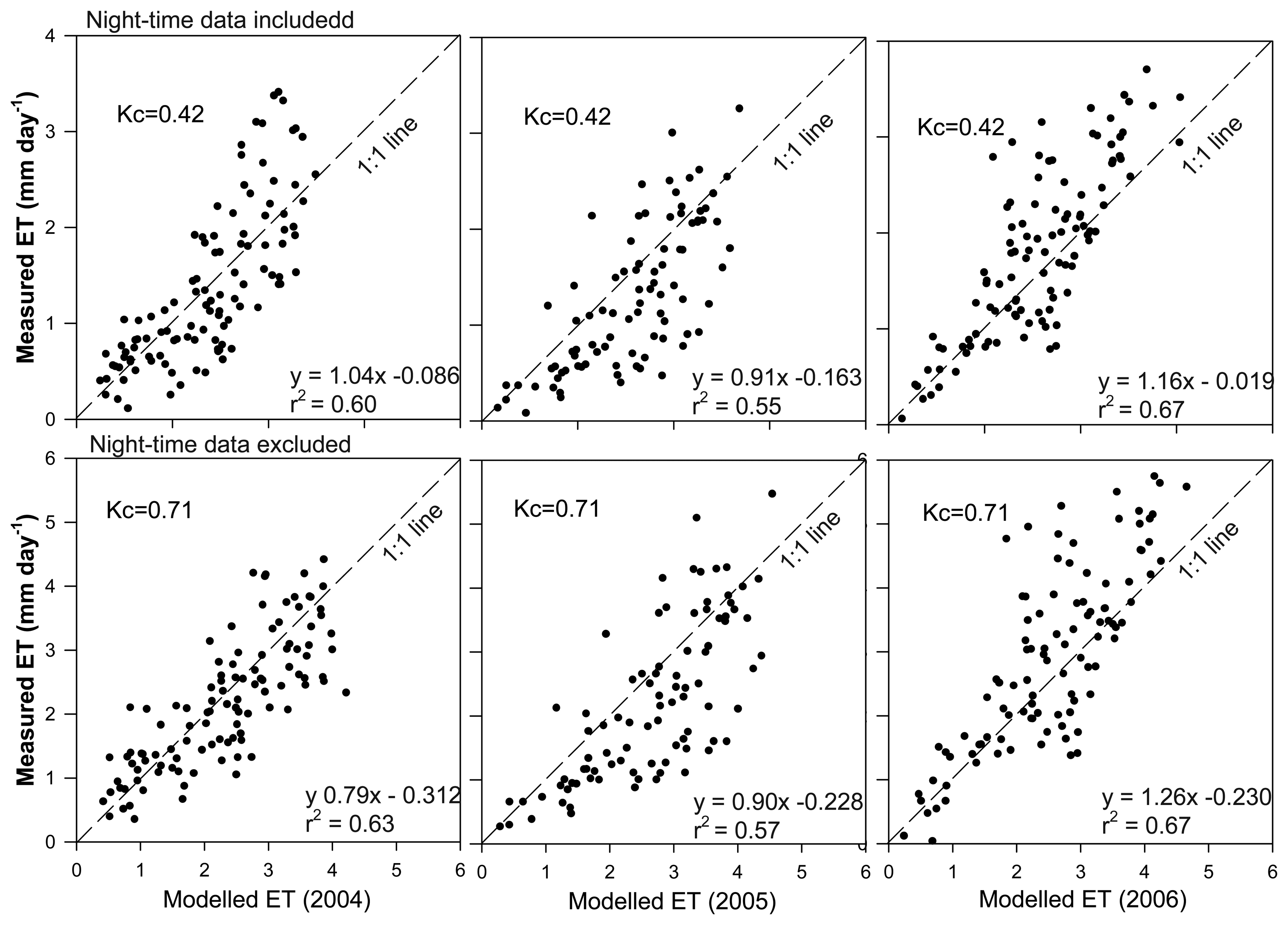
3.4. Inter-annual variability of model performance

All three models showed slight variability between years. As an example, the results between the PM calculated ET with and without night-time data and the measured ET for 2004 to 2006 are presented in Figure 6. Generally speaking, better performance of model was achieved with night-time data for the specific year. After the night-time data were removed, a higher r² was obtained for the year 2004 and 2005, but the slope decreased and intercept increased. This finding indicates that removing night-time data may not be necessity if the BR data is used for validating ET models in this region when the PM method is used.

3.5. A comparable validation of the tested model using the data collected in 2007

To further compare the performance of different models, a dataset collected during a short period (Julian Day 220-260) of year 2007 was analyzed. In this case study, fixed Kc values derived from the data collected in the previous 3 years (2004-2006) were applied to different models, i.e, 0.42 for the PM method, 0.44 for the PT method, and 0.67 for the PE method, respectively. The results are shown in Figure 7. All of the tested models gave a good fit to the dataset with a r²>0.6. The single factor analysis in

Table 3. A comparison between different methods with data collected during 2007*.

Methods*	Number	Mean	Variance	P**	F***	Fcrit	RE(%)****
PM	40	1.42	0.33	0.53	0.40	/	6.05
PT	40	1.45	0.55	0.43	0.62	/	8.70
PE	40	1.52	0.50	0.20	1.70	/	13.94
ET	40	1.34	0.34	1	/	3.96	0

^*see footnote of table 1 for explanation of each letter in the table

indicated that there was no significant difference between measured ET and the modeled ET by applying the corresponding Kc. The relative bias of the modeling is 6.5% for the PM, 8.7% for the PT, and 14% for the PE, respectively. All of the tested equations achieved very good agreement with the measurement value. However, the PT method seemed to be better in both intercept and slope. The PT method also had the least requirement of input variables and could be recommended for future application in estimating evapotranspiration in this region.

3.6. A further refinement the PT method in the region

The PT method has been found to perform better in other regions [10]. The method also has a constant which can be refined or calibrated based on the local data. For example, other authors [36;37] suggested different α parameter values of 0.8 and 1.2. To test possibly suitable values of this parameter for this region, a dataset collected during 2007 was used to find the best constant for the region. By applying a Simplex and Least square error fitting technique we found that the α-value should be within a range of 0.8∼2.0 with 1.28 being the best estimate. This is slightly higher than the commonly used α-value (1.26).

4. Conclusions

Although three tested methods provides good agreement with the observation (r²>0.6), the PT method has been recommended for future application in this region because its simplicity and consistent performance. A further optimization revealed that a α constant value of 1.28 in the PT equation made the model perform well for this region

The BR method has been found to provide a reasonable estimation of ET for this region. Normally, 20% of BR observation must be rejected because of many reasons related to wetness, unstable atmospheric condition, and others.

Crop coefficient (Kc) varied from day to day with a range of 0.2 to 1.4 depending on the methods used to calculate reference ET. After summarizing 3 years of observation, it has been found that values of 0.42, 0.44, 0.67 could be used for the PM, PT, and PE, respectively, to provide a good mean estimation of ET for this region. The Kc value also showed certain degree of variation from month to month, due to the phonological condition of the crop development.

The BR observations indicated that the average ET in the Fredericton area of New Brunswick was 2.5 mm day^-1 during Julian Day 164-274. However, the ET varied with time and the specific climatic conditions.

References

1. López-Urrea, R.; Martin de Santa Olalla, F.; Fabeiro, C.; Moratalla, A. Testing evapotranspiration equations using lysimeter observations in a semiarid climate. Agricultural Water Management 2006, 85, 15–26. [Google Scholar]
2. Allen, R.G.; Pereira, L.S.; Raes, D.; Smith, M. Crop Evapotranspiration.Guidelines for Computing Crop Water Requirements; FAO: Rome, Italy, 1998; FAO Irrigation and draiange, Paper No. 56. [Google Scholar]
3. Hargreaves, G.H.; Samani, Z.A. Reference crop evapotranspiration from temperature. Applied Engineering Agriculture 1985, 1, 96–99. [Google Scholar]
4. Jensen, M. E.; Burman, R. D.; Allen, R. G. Evapotranspiration and irrigation water requirements; Committee on Irrigation Water Requirements of the Irrigation and Draniage Division of ASCE: New York, 1989. [Google Scholar]
5. Droogers, P.; Allen, R.G. Estimating Reference Evapotranspiration Under Inaccurate Data Conditions. Irrigation and Drainage Systems 2002, 16, 33–45. [Google Scholar]
6. Penman, H.L. Vegetation and hydrology. In Technological Communication 53; Commonweath Bureau of Soils: Harpenden, England, 1963. [Google Scholar]
7. Allen, R.G.; Jensen, M.E.; Wright, J.L.; Burman, R.D. Operational estimates of reference evapotranspiration. Agronomy Journal 1989, 81, 650–662. [Google Scholar]
8. Steiner, J.L.; Howell, T.A.; Schneider, A.D. Lysimetric evaluation of daily potential evapotranspiration models for grain-sorghum. Agronomy Journal 1991, 83, 240–247. [Google Scholar]
9. DehghaniSanij, H.; Yamamoto, T.; Rasiah, V. Assessment of evapotranspiration estimation models for use in semi-arid environments. Agricultural Water Management 2004, 64, 91–106. [Google Scholar]
10. Priestley, C.H.B.; Taylor, R.J. On the assessment of surface heat-flux and evaporation using large-scale parameters. Monthly Weather Review 1972, 100, 81–92. [Google Scholar]
11. Xing, Z.; Chow, L.; Meng, F-R.; Rees, H.W.; Lionel, S.; Monteith, J. Testing reference evapotranspiration estimation methods using evaporation pan and modeling in Maritime region of Canada. Journal of Irrigation and Drainage Engineering 2007, in press. [Google Scholar]
12. Blad, B.L.; Rosenberg, N.J. Lysimetric calibration of the Bowen Ratio-Energy Balance method for evapotranspiration estimation in the central Great Plains. Journal of Applied Meteorology 1974, 13, 227–236. [Google Scholar]
13. Ashktorab, H. Partitioning of evapotranspiration using lysimeter and micro-Bowen-ratio system. J. Irrig. and Drain. Engrg. 1994, 120(2), 450–464. [Google Scholar]
14. Yrisarry, J.J.B.; Naveso, F.S. Use of weighing lysimeter and Bowen-Ratio Energy-Balance for reference and actual crop evapotranspiration measurements. ISHS Acta Horticulturae 2000, 537. [Google Scholar]
15. Viana, T. V.; Folegatti, M. V.; Azevedo, B. M.; Bomfim, G. V.; Elói, W. M. Evapotranspiration through the Bowen ratio system and a weiching lysimeter in greenhouse. IRRIGA 2003, 8(2), 113–119, in Spanish. [Google Scholar]
16. Fontenot, R.L. An evaluation of reference evapotranspiration in Lousiana; Louisiana State University and A&M College, 2004; pp. 1–83. [Google Scholar]
17. Villar, J.M. Adjusting reference ET using local calibrations by means of a Bowen ratio system; 1992. [Google Scholar]
18. Malek, E. Calibration of the Penman wind function using the Bowen ratio energy balance method. J. Hydrol. (Amst.) 1994, 163(3-4), 289–298. [Google Scholar]
19. Peacock, C.E.; Hess, T.M. Estimating evapotranspiration from a reedbed using the Bowen ratio energy balance method. Hydrological Processes 2004, 18, 247–260. [Google Scholar]
20. Todd, R.W.; Evett, S.R.; Howell, T.A. The Bowen ratio-energy balance method for estimating latent heat flux of irrigated alfalfa evaluated in a semi-arid, advective environment. Agricultural and Forest Meteorology 2000, 103, 335–348. [Google Scholar]
21. Gavilan, P. Accuracy of the Bowen ratio-energy balance method for measuring latent heat flux in a semiarid advective environment. Irrigation Science 2007, 25(2), 127–140. [Google Scholar]
22. Ohmura, A. Objective criteria for rejecting data for Bowen ratio flux calculations. Journal of Applied Meteorology 1982, 21, 595–598. [Google Scholar]
23. Angus, D.E.; Watts, P.J. Evapotranspiration--how good is the Bowen ratio method? Agricultural Water Management 1984, 8, 133–150. [Google Scholar]
24. Unland, H.E.; Houser, P.R.; Shuttleworth, W.J.; Yang, Z.L. Surface flux measurement and modelling at a semi-arid Sonoran Desert Site. Agricultural and Forest Meteorology 1996, 82, 119–153. [Google Scholar]
25. Perez, P.J.; Castellvi, F.; Ibañez, M.; Rosell, J.I. Assessment of reliability of Bowen ratio method for partitioning fluxes. Agricultural and Forest Meteorology 1999, 97, 141–150. [Google Scholar]
26. Ortega-Farias, S. O.; Rojas, V.; Valdés, H.; Gonzaléz, P. Estimation of reference evapotranspiration in the Maule Region of Chile: a comparison between the FAO Penman-Monteith and Bowen ratio methods. Acta Horticulturae 2004, 664, 469–475. [Google Scholar]
27. Bowen Ratio Instrumentalion Instruction Manual; Campbell Scientific Inc., 1995.
28. Suleiman, A.A.; Hoogenboom, G. Comparison of Priestley-Taylor and FAO-56 Penman-Monteith for daily reference evapotranspiration estimation in Georgia, USA. Journal of Irrigation and Drainage Engineering 2007, 133(2), 175–182. [Google Scholar]
29. Stannard, D.I. Comparison of Penman-Monteith, Shuttleworth-Wallace, and modified Priestley-Taylor evapotranspiration models for wildland vegetation in semiarid rangland. Water Resources Management 1993, 29(1993), 1379–1392. [Google Scholar]
30. Li, L.; Yu, Q. Quantifying the effects of advection on canopy energy budgets and water use efficiency in an irrigated wheat field in the North China Plain. Agriculture and Water Management 2007, 89, 116–122. [Google Scholar]
31. Nichols, J.; Eichinger, W.; Cooper, D.I.; Prueger, J.H.; Hipps, L.E.; Neale, C.M.U.; Bawazir, A.S. Comparison of evaporation estimation methods for a riparian area. Final report. In UHR Technical Report No. 436; College of Engineering, University of Iowa: USA.
32. Bowen, I.S. The ratio of heat losses by conduction and by evaporation from any water surface. Physics Review 1926, 27, 779–787. [Google Scholar]
33. Tanner, C.B. Energy balance in approach to evapotranspiraiton from crops. Soil Science Society of America Proceedings 1960, 24, 1–9. [Google Scholar]
34. Verma, S.B.; Rosenberg, N.J.; Blad, B.L. Turbulent exchange coefficients for sensible heat and water vapor under advective conditions. Journal of Applied Meteorology 1978, 17, 330–338. [Google Scholar]
35. Allen, R.G.; Hill, R. W.; Srikanth, V. Evapotranspiration parameters for variably sized wetlands. America Society of agricultural and Engineering 1994, 94, 21–32. [Google Scholar]
36. Green, A.E. Evapotranspiration from pasture: a comparison of lysimeter and Bowen ratio measurements with Priestley-Taylor estimates. New Zealand Journal of Agricultural Research 1984, 27, 321–327. [Google Scholar]
37. Sumner, D.M.; Jacobs, J. M. Utility of Penman-Monteith, Priestley-Taylor, reference evapotranspiration, and pan evaporation methods to estimate pasture. evapotranspiration. Journal of Hydrology 2005, 308, 81–104. [Google Scholar]
Figure 1. Daily pattern of data rejection frequency (0∼1) and wind speed (m/s) (a); data rejection rates over different discard rate for different reasons (b).
Sensors 08 00412f1
Figure 2. Diurnal cycle of Evapotranspiration.
Sensors 08 00412f2
Figure 3. A comparison between measured (all data included) and modeled ET.
Sensors 08 00412f3
Figure 4. A comparison between modelled and measured ET (night-time data are excluded).
Sensors 08 00412f4
Figure 5. Kc variability over time. PM, PT, and PE stand for the Penman-Monteith, Preistley-Taylor, and Penman 1963, respectively, when the Kc Values were calculated with night-time data. PM2, PT2, and PE2 stand for the Penman-Monteith, Preistley-Taylor, and Penman 1963, respectively, when the Kc Values were calculated with night-time data removed.
Sensors 08 00412f5
Figure 6. Variability of the performance of the PM model in different years. In the top panel, night-time data were included with Kc = 0.42. In the bottom, night-time data were excluded in calculation, Kc = 0.71. The number in the bracket indicates the year.
Sensors 08 00412f6
Figure 7. A comparison of the model performance, applying Kc values derived from year 2004-2006 into the data collected during 2007. PM stands for the Penman-Monteith method, PT, for the Priestley-Taylor; and PE, for the 1963 Penman Equation. The numbers in the brackets after each method name are the Kc vlues used.
Sensors 08 00412f7