1. Introduction: Overall Description
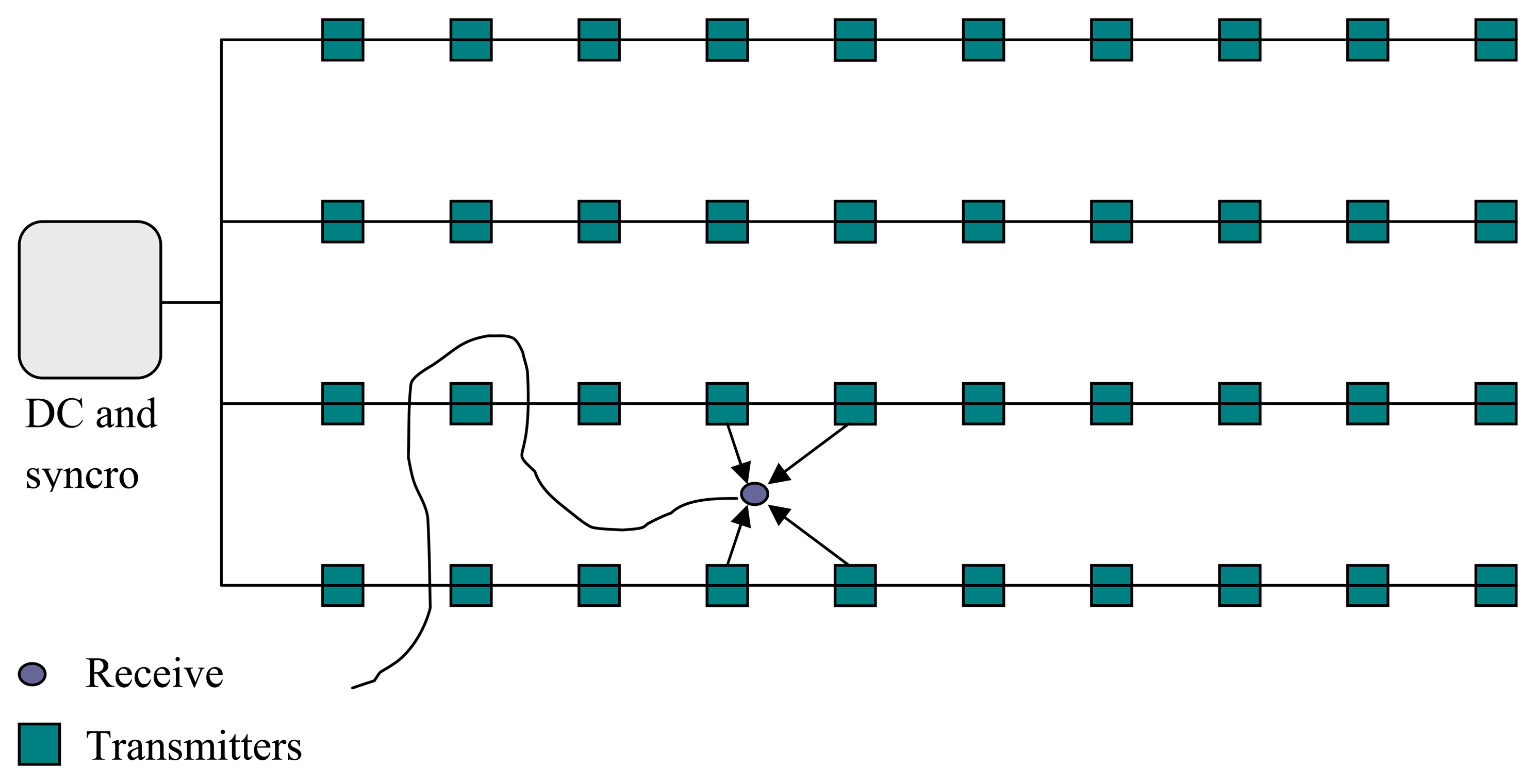
First of all a network of transmitters is connected, not necessarily in a regular form, and positioned at different heights. All are fed from a common source which synchronises the common time signal of 1 Hz as is shown in
figure 1. Each transmitter is capable of remembering its identity code which has to be unique within its range of operation, together with the strength of the signal transmitted which varies according to its height. In order to be able to change this configuration easily, the transmitter has an infrared receiver based on the popular band of domestic remote controllers.
As will be seen later, the number of transmitters depends on the time lapse of the modulated code in the ultrasonic band, the distance between transmitters and the limit defined by the passing of one second, during which time all the transmitters must emit their codes. This is not the case of the receivers. There is no maximum number because they act independently of each other. For this reason only one receiver is considered form now on. Essentially the receiver is an intelligent sensor that consists of an ultrasonic transducer centred on the 40 KHz band, sealed in order to make it as resistant as possible to use, and a microcontroller which decodes a modulated frame modifying the threshold dynamically and applying processing techniques to cancel bouncing interference [
6]. The sealed restriction significantly increases the gain of the input amplifier.
The whole system needs to know the course of the receiver which in the GPS system[
1] is obtained from two position measurements at different times as long as there is movement. Since, in this case, the position measurements are obtained every second, the user moves slowly and, as a final touch, the orientation of the receiver does not necessarily coincide with the direction of movement, it was necessary to develop a system to detect the orientation of the receiver [
1]. Of the two available ways of resolving these problems- the gyroscope and the magnetic compass- it was decided to use the latter based on two Hall-effect linear transducers. The accuracy of this method is poor – plus or minus 15 degrees- but is sufficient for this purpose.
In the following pages each of the components which make up the system will be analysed, starting with the generator of the main clock, continuing with the transmitter and finishing with a description of the receiver, where we will be seen the system impulse response, the design of the input amplifier and the frame detection circuit. Following that is the description of the test scenarios, the trials of sensitivity, the determination of the radius of reception, the intersymbolic interference caused by signals reflected off nearby walls and of the algorithms which correct the sources of error.
2. General Clock Generation
In
figure 2 can be seen the blocks of the generator of the time signal. It receives DC voltage from the power source and the DC switch block interrupts the source at the rhythm imposed by the “Enable” signal. This signal is generated in the “Clock Generation” block.
The natural condition of “Enable” is logical one during most of the time but every second it changes to zero for 16 ms. Looking at
figure 3 it can be seen that for most of the time Q4 is “On” so that Q1 will also be “on” as long as the entry voltage is more than 12V plus the threshold voltage, V
GS, of Q1, that is 15V.
At the exact moment that “Enable” falls to zero, Q1 cuts off and Q3 starts to conduct. Since the transmitters have a significant entry capacity (100nF each one, for 1000 transmitters in the average system, gives a combined capacity of 100uF) it is necessary to use a resistance which can absorb the energy of all these condensers. R2, together with Q3, completes an RC network with an accuracy of 1.5ms in the average installation, ten times less than the duration of the “Not Enable” pulse. Without Q2, the static capacity between the Gate and the Source of Q1 would prevent it changing to “off” quickly enough to avoid an unnecessary flow of current to R2 [
5].
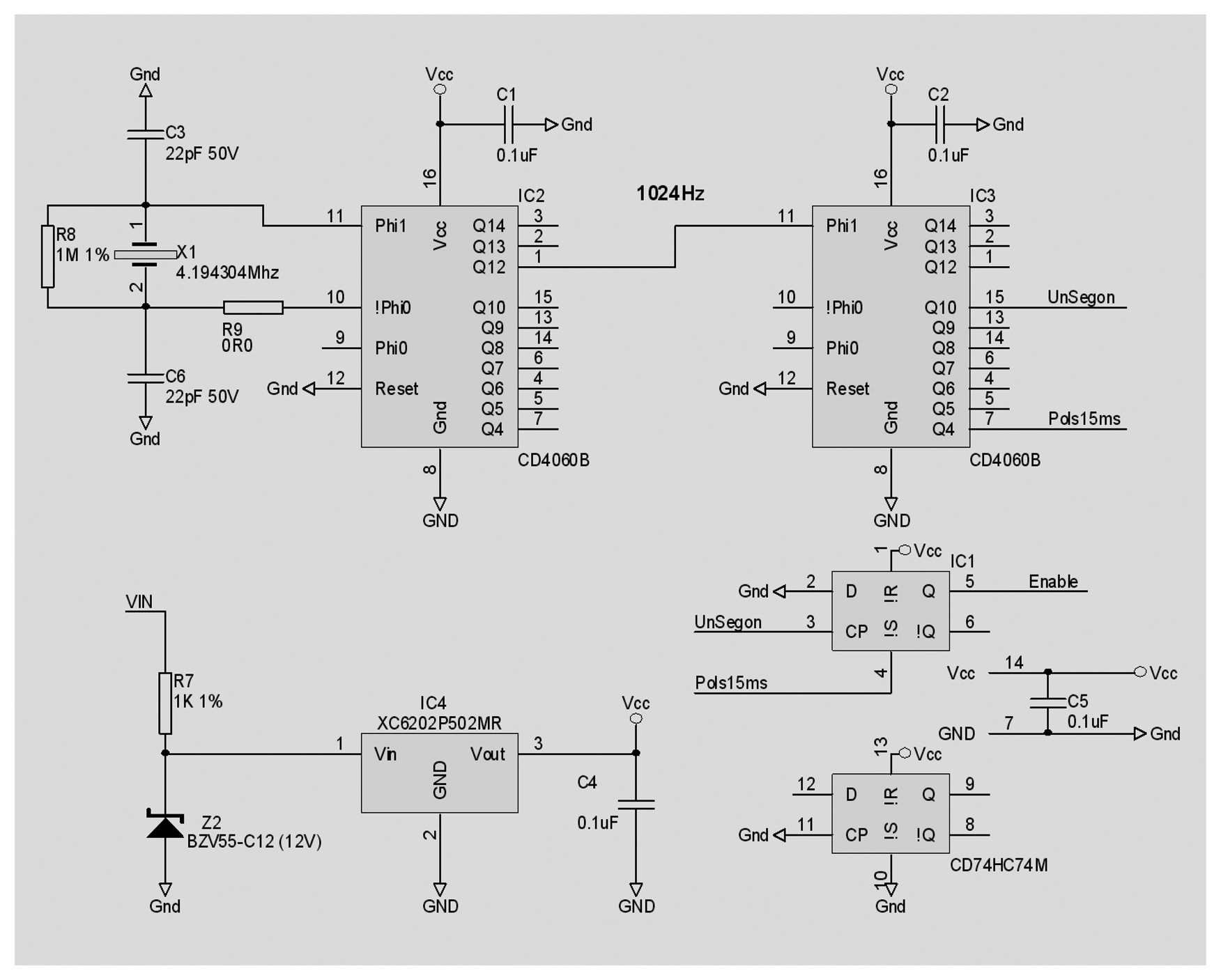
The second block consists of the actual clock which creates the “Enable” signal as can be seen in
figure 4. A crystal of 4.19430Mhz is divided by 4096 at point IC2 which generates a frequency of 1024Hz which is then divided again, this time by 1024, thanks to IC3. The exit point Q4 of this integrated circuit produces a pulse of 15.625 ms as a by-product of the division of 1024 by 64. Finally the ICI flip-flop combines the two signals to create the “Enable” exit, the wave form of which is shown in
figure 5.
Since the consumption of each transmitter is known to be 20mA on average and a typical installation consists of 1000 transmitters, this device was designed to allow 2A to pass through without needing to add cooler to the transistors at Q1 and Q3. Effectively the power absorber in Q1 hardly reaches 300mW which, with a thermal resistance union-ambient of 62.5, only increases its temperature by 17 degrees. Similarly Q3 discharges a capacity of 100uF via a 15Ω resistance in 1ms which, in an average of 1 second, produces a 2.5mA current and can be ignored.
As a result the whole synchronising mechanism can be positioned in a printed circuit as shown in
figure 6.
3. The Ultra Sound Transmitter
3.1. Block diagrams
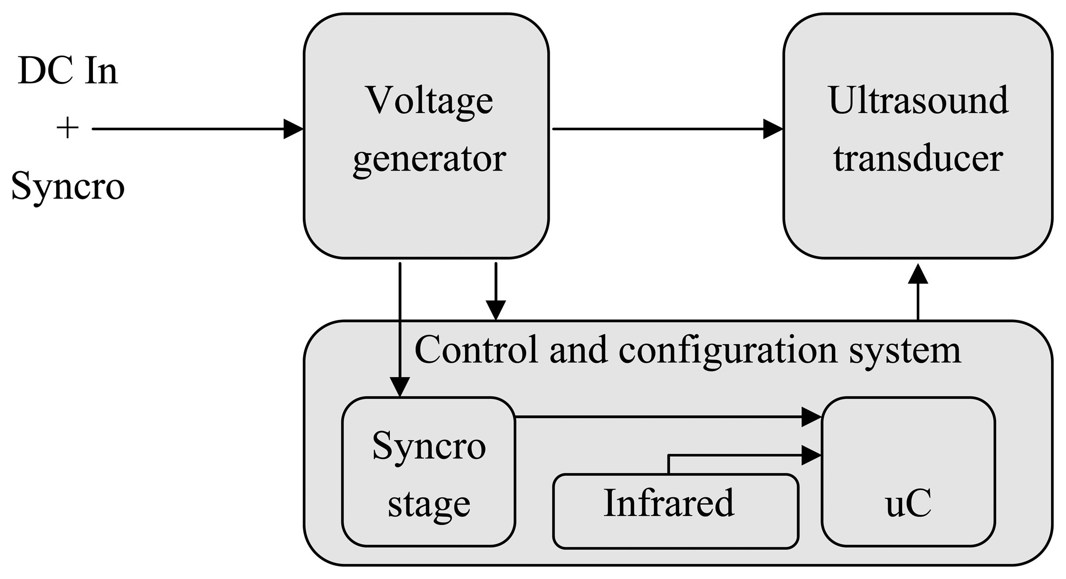
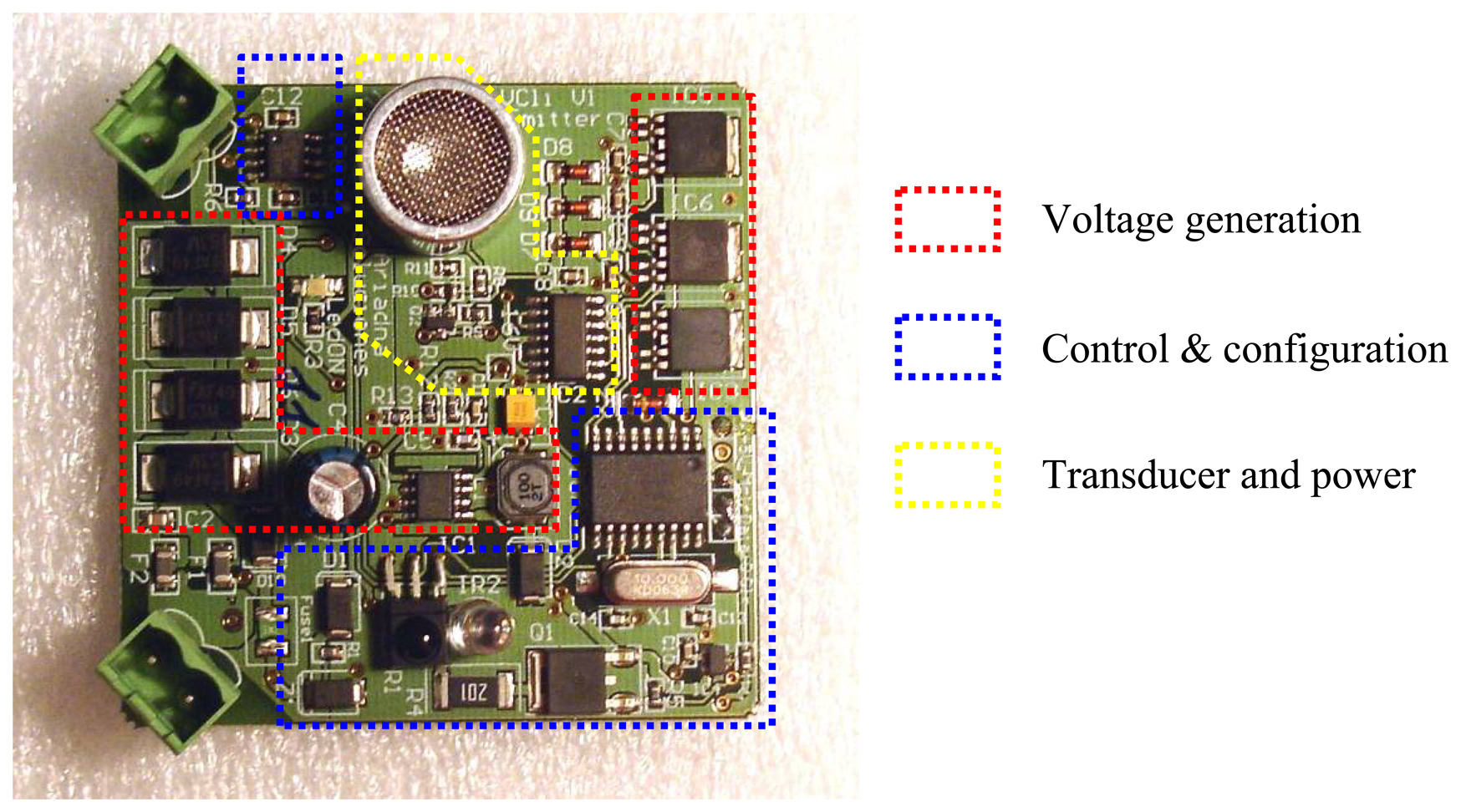
As can be seen in
figure 7, the ultrasound transmitter consists of 3 blocks- the voltage generator, the ultrasonic transducer and the control and set-up system.
3.2. Voltage generation
This unit receives a constant supply of 24V with the synchronised clock overloaded and creates a rectified voltage (D3, D4, D5 and D6) independent of the input polarity, and filter it in differential mode (F12, F2, F3). This filter is not designed to increase the conductive immunity of the transmitter but to reduce the noise level which the ICI regulating switch can introduce into the 24 V network. To prevent any anomalous electronic occurrence in the transmitter from causing a short-circuit in the whole 24V network, a fuse (fuse 1) was added. Since this fuse can be re-triggered, it allows the shock wave passing through the 24V network to be absorbed by Z1 without causing a permanent malfunction as would happen with conventional fuses.
From here the “!Sincro” signal is obtained and sent to the clock's detection circuit. It also provides the voltage which the Step Down (ICI) regulates to a value of 16V with 95% efficiency. This voltage level protects against the variations possible when the full 24V net is deployed, generates the voltage of the microcontroller at IC4 and of the 3 linear regulators IC3, IC5 and IC6. These last three supply the ultrasound transducer's power via the control signals “!Enable 5V”, “!Enable9V” and “!Enable12V” which switch on one of the 3 regulators according to the height at which the transmitter is installed. The need to control the voltage of the transducer according to the height of the installation is discussed in section 4. It will suffice at this stage to say that if the distance between the transmitter and the receiver is too short, the receiver's amplifier can become overloaded [
3][
4].
3.3. The ultrasound transducer
The choice of an ultrasound transducer operating in the 40 KHz band and not another one was decided on the grounds of availability and variety because of the existence of a large number of manufacturers and models [
3][
4]. The different models easily available in the European market were analysed and the main deciding factor was the breadth and uniformity of the beam of radiation. The need for a wide beam of radiation is shown in
figure 9. It can easily be seen that the radius of reception of a transmitter increases as the beam of radiation increases [
3]. It is also evident that the greater the radius, the fewer transmitters are required for a given area.
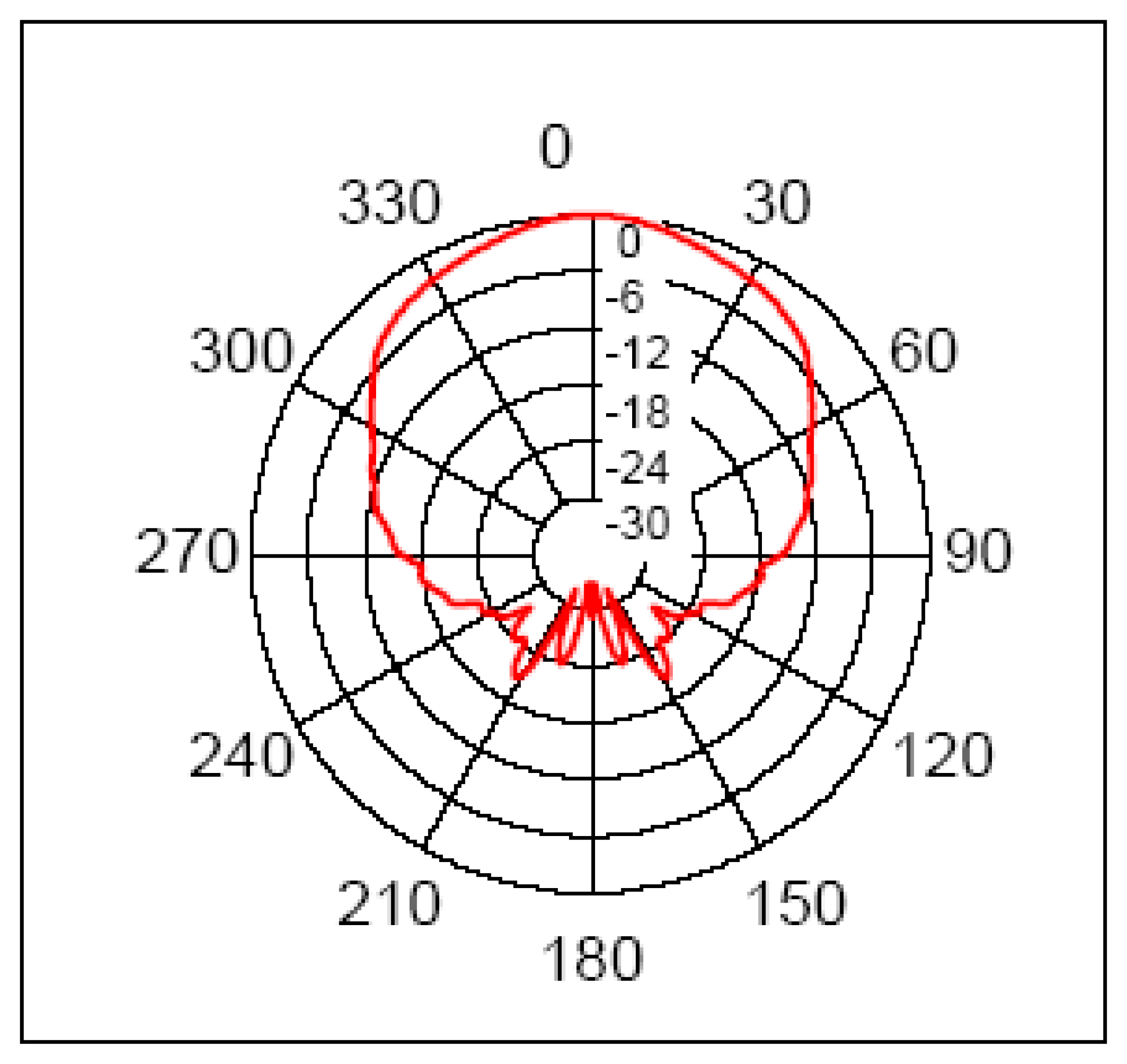
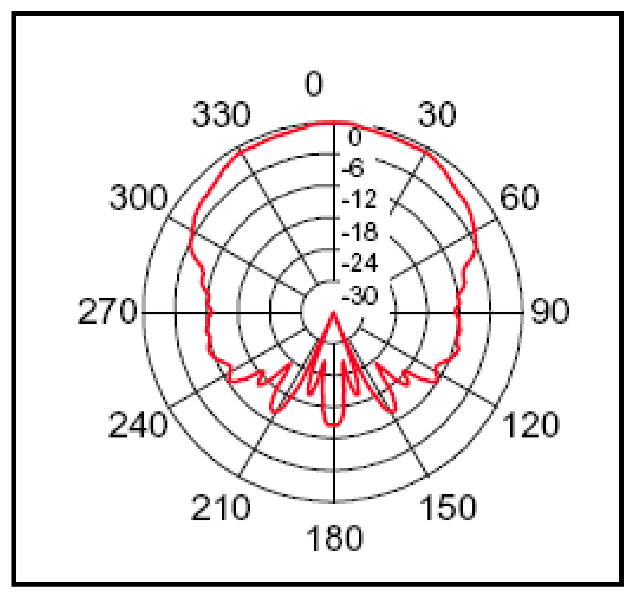
The transducer which met the requirements best was Model 400ST120, distributed by Midas Components Ltd.
Figure 10 shows its beam of radiation and it can be seen that at 45 degrees the loss suffered hardly reaches 3dB.
This kind of transducer is based on a piezoelectric properties crystal [
3] with a mechanical resonance frequency centred on 40KHz. To achieve a change in air pressure which produces an acoustic wave, it is only necessary to apply a change in voltage to the transducer's terminals. Clearly, new impulses produce new waves. From the electronic point of view the transducer behaves like a condenser with small traces of induction and resistance which are negligible for this purpose.
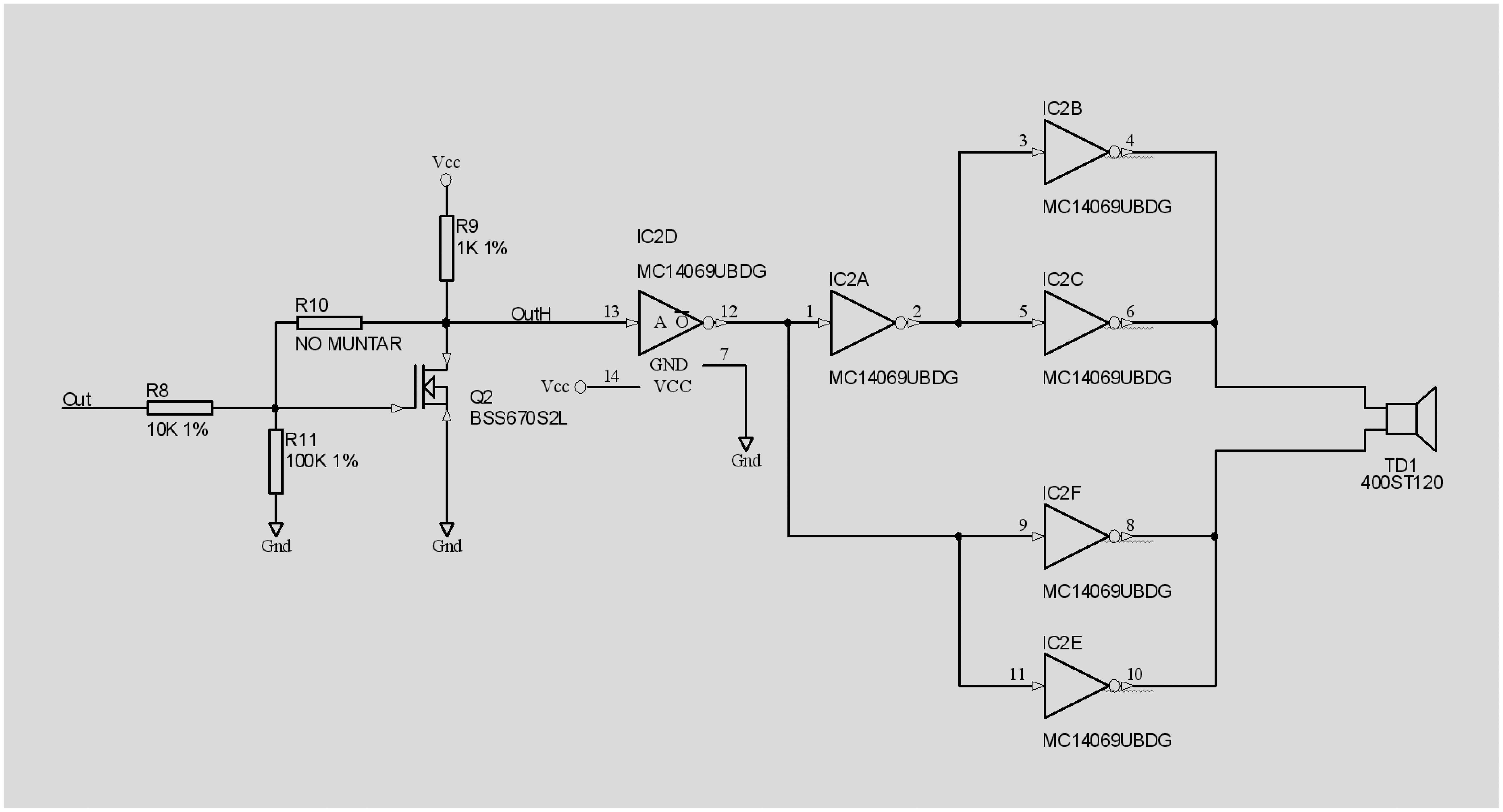
Later the format of the information sent by the transmitter via the transducer will be discussed. For the time being, only the power phase described in
figure 11 will be studied. It can be seen that the “Out” signal coming form the micro-controller is applied to a level shifter (the micro-controller works with 5V) based on Q2 to increase it up to the IC2 supply level. The choice of a CMOS hex inverter as the exit stage is justified because of the range of voltages with which it can work (from 3 to 18V) and its adequate output current capability– both source and sink [
5].
To estimate the current the inverters need to supply, it should be remembered that the supply can be 5V, 9V or 12V according to what the micro-controller decides in the “!Enable5V”, “!Enable9V” and “!Enable12V” signals and sends to the voltage generator [
3][
4]. Given the well-known formula C=Q/V or C = ΔQ / ΔV, it will be noted that the higher the voltage, the greater the power fed to the condenser, as long as it is possible to maintain the current required by the capacitor. The chosen transducer has a nominal capacity of 2.4nF and the duration of a pulse is 25us. If the time required for an falling and rising is 2us in the worst case i.e. 12V, then the current needed is Δi= 2.7nF·12V / 2us or 15mA. Since each inverter is capable of delivering 8.8mA, it was decided to put two in parallel which also stimulate the TD1 transducer in counter phase, thanks to IC2A. The shape of the wave delivered by the inverters is shown in
figure 12. Note that the amount detected by the transducer is twice the supply voltage of IC2, in this case 12V.
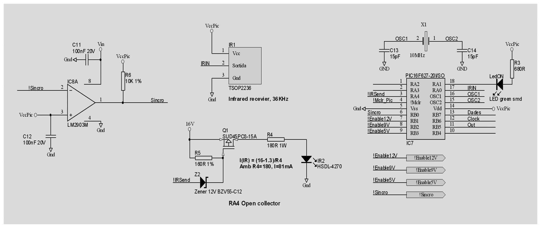
3.4. The control and configuration system
The control system is based on Microchip's PIC16F627 microprocessor which executes the program which sends the transmitter's code to the ultrasound transducer. The microprocessor stores in its EEPROM 2 parameters which it receives from the infrared receiver – the voltage of the emission and the transmitter's identifier code. In principle, this information is only needed the first time the system is switched on, via an infrared signal sent by an authorised operator to each of the transmitters. According to the configured power level, the microcontroller will activate one of the three voltage control signals “!Enable5V”, “!Enable9V” or “!Enable12V”.
Figure 13 shows the diagram of the 3 parts which make up this complete block. Firstly, on the right-hand side, is the unit which detects falls in the supply voltage every second and sends them to the microprocessor as the source for synchronisation. The detection point is influenced by the equivalent capacity which the supply voltage presents and is a function of the place occupied by the transmitter in the network. Clearly this is a possible source of error which is called “Capacity variation error”, but it is not the only one.
The microcontroller, on receiving the synchronising signal, starts a time count which depends upon the transmitter's identity code. The delay from the main clock synchronisation to the transmitting of the message frame by every transmitter is:
The 24 ms which the software uses as its time-base comes from the need to establish a security distance between two transmitters which, in the case of two set up at the maximum height with the capacity to contact a receiver means that their signals never collide. The integer remainder operator (mod) applied to the identifier limits the account to 32 possible delays, which makes it possible for two identifiers with the same integer remainder of 32 (that is they are synonymous) to be seen by the same receiver. Evidently this should not happen but it is not a very important restriction because it is possible to separate the synonymous identifiers by double the nominal range so that they are invisible to each other. The accuracy of the
equation (1) time count depends exclusively on the accuracy and deviation of crystal X1 which in turn produces the “Error in the start-up phase”. It is worth noting that this error is minimised, though not eliminated, by choosing for X1, a model with an accuracy of 20ppm and thermal deviation.
Remembering that in reality there are only 32 different transmitters, these only occupy 768ms of each 1000ms which makes up the synchronisation period i.e. 32×24ms. This apparently unused time window is used to enable the interruptions received by the infrared reader and to be able to deal with the eventual reception of new configuration values. Outside this reception window, the microcontroller only deals with the timing interruptions and the internal timer. In this way the uncertainty of interruption is limited to 500ns, the effect of which is so small that it does not feature in the list of sources of error.
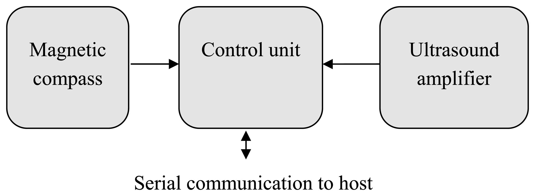
4. Description of the Ultrasound Receiver
The receiver consists of three blocks- the ultrasound amplifier, the electronic compass and the control unit as shown in
figure 15.
It can be seen that the control unit communicates with a host whose computing capacity is much greater because, in order to calculate the position, it is necessary to calculate a series of operations with double float accuracy and subject several trigonometric routines [
1][
12]. The receiver only detects and retransmits the identifier codes that the receivers it receives in one second and the time gap between them. This information, together with the direction obtained from the magnetic compass is sent to the host every second. The host, since the position of all the transmitters is known and the height is constant, can eliminate the uncertainty caused by the difference between the receiver's clock and the standard synchronisation, and also calculate the actual speed of the sound by successive approximations [
1]. Unfortunately it is not possible to study the description of the algorithms which execute the software in this paper for reasons of space. Neither is the design of the magnetic compass studied but it is worth noting that it contains nothing new for it consists of the classic pair of Hall-effect sensors set up in 90 degrees [
11][
5].
4.1 Ultrasound amplifier
4.1.1 Overall description
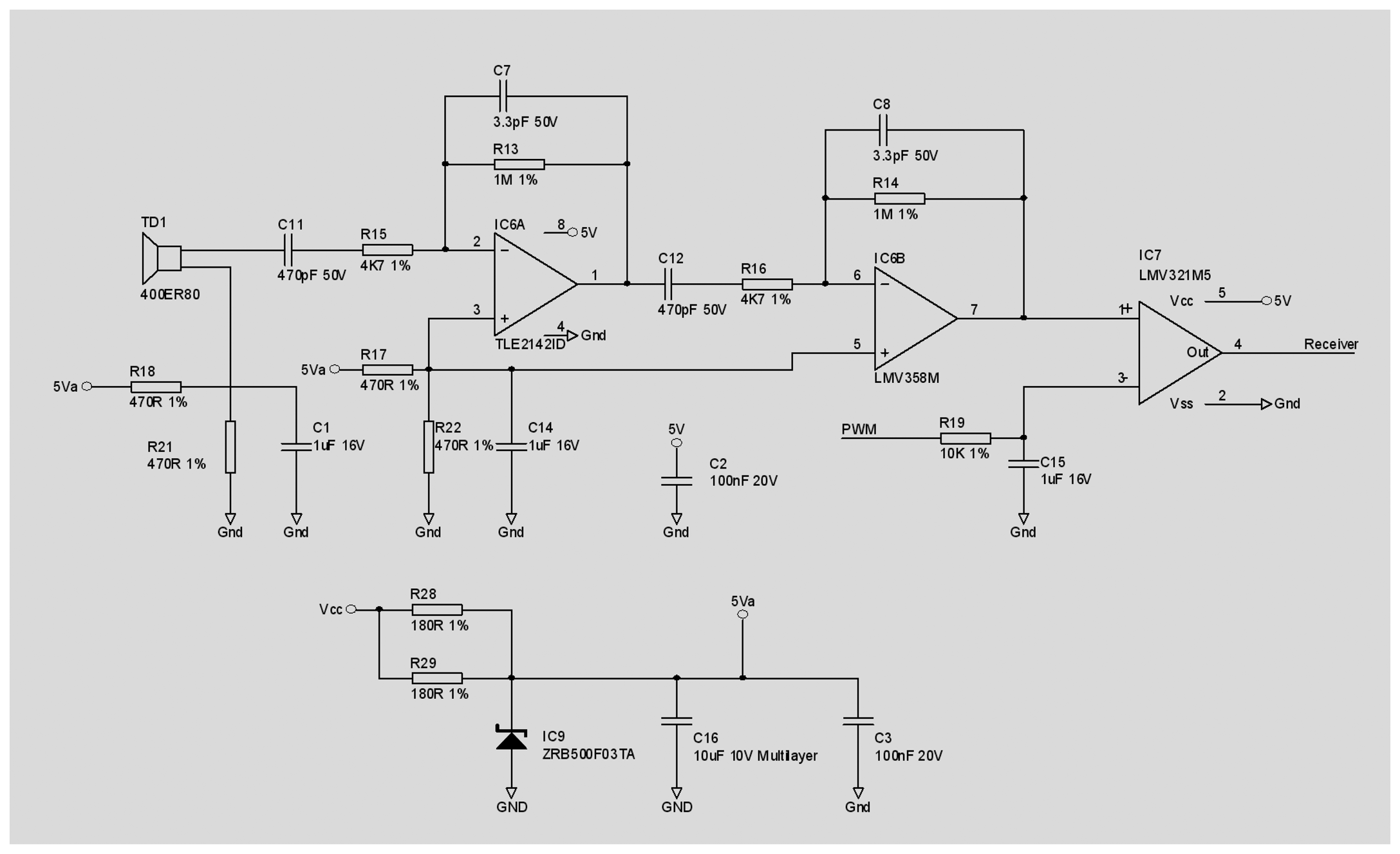
Figure 16 shows the amplifier and the design works with an asymmetrical of 0 to 5V which means special attention must be paid to polarising the inputs of the operational amplifiers to the centre of the common permissible mode [
5], that is 2.5V. Having said this, the amplification circuit will now be considered, starting with the virtual ground which is generated from the voltage of 5V, firmly decoupled from the entry voltage and divided in two by the R17-R22 and R18-R21 separators. At both points there is 2.5 V, a relatively low impedance and ceramic decouplers of 1uF, which enable the non-inverting inputs of the two operational amplifiers contained in IC6 to be digital noise isolated. This amount of resources to obtain a virtual ground is due to the fact that the final result of the ultrasound amplifier is a digital signal which changes at the same rhythm as the signal received by the transducer. Experience shows that if the virtual ground is not firmly decoupled from the input voltage, the digital output is seen in the entry signal and generates positive feedback and, therefore, oscillations in the whole circuit [
5].
The waves received by the TD1 transducer are filtered and amplified by IC6A and IC6B, which are configured as a pass band amplifier centred on 40 KHz and produce a gain of 70dB – later the need for such a gain will be discussed. Finally they are connected to a measuring device, the reference level of which can be changed by the micro-controller thanks to a PWM outlet which is filtered by R19-C15 to obtain a DC level proportional to the Duty Cycle of the PWM output. Because of lack of choice the TIE2142 was chosen for its low noise level, an essential property for handling such a high gain.
4.1.2 The transducer
The same parameters for the transmitter were used to choose the transducer i.e. a wide reception area, availability, reasonable price and, in addition, sealed. Sealed transducers have lower reception sensitivity than open ones for obvious reasons. The result of the search was model 400ER080 made by the same manufacturer as the transmitter and the reception beam of which is shown in
figure 17 which shows that at 45 degrees the reduction in nominal sensitivity is only -3dB.
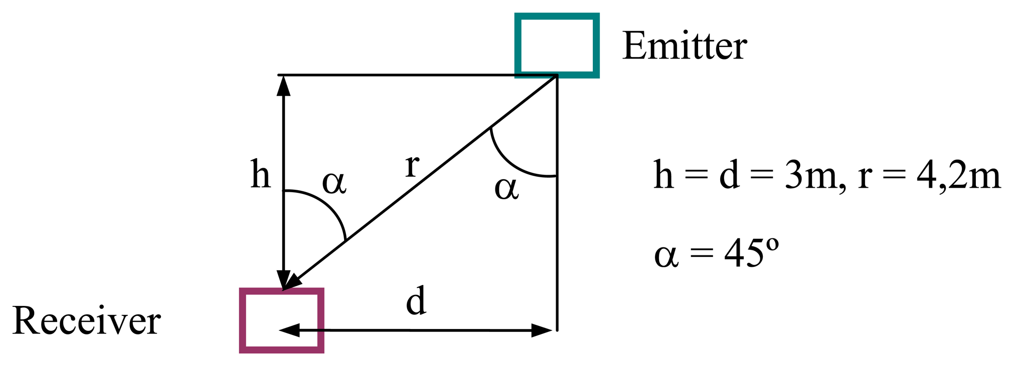
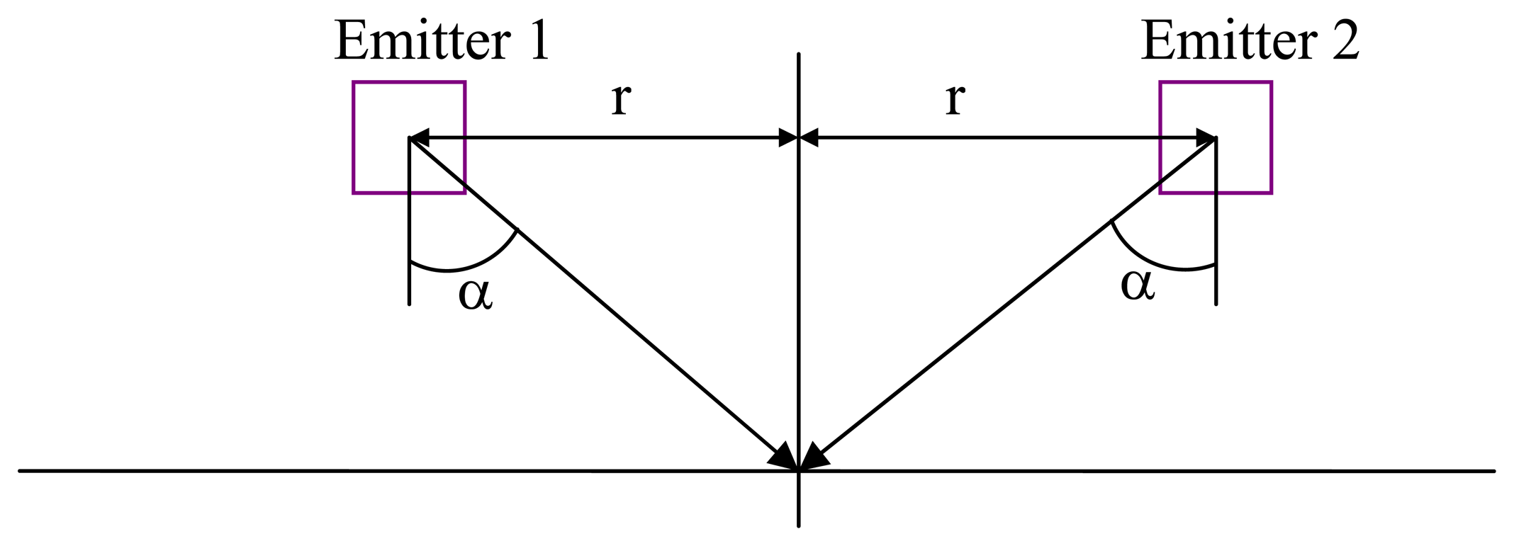
The calculation of the gain must take into account the worst case scenario [
3], which is when the receiver is not vertical to the transmitter. The working limit of the average set-up which is expected to be found in places where this solution is installed is considered to be an angle of 45 degrees and a distance of three metres between transmitters situated three metres above the receiver, as shown in
figure 18.
In these conditions and given the following data, taken from the manufacturer's specifications, the first estimate of the gain from the amplifier was made.
Transmitter:
- a)
Sound pressure level at 40KHz: 10Vrms a 30cm; 0dB re 0.0002μbar
- b)
SPL a 40Khz = 120
Receiver:
- a)
Sensitivity of the receiver at 40KHz: -75dB; 0dB = 1V/μbar
Knowing that the pressure decrease with the distance at the rate of 1/r [
3], it is possible to deduce [
2] that the pressure present in the output of the transducer of the receiver, in the worst case shown in
figure 18, starting from the pressure at distance r from the transmitter:
Where the factor 0·707 corresponds to the fall of -3dB which the transmitter suffers at 45 degrees. Now it is possible to calculate the voltage present at the transducer's output:
Fixing an output of 1V maximum as the worst case, in order to obtain a margin of up to 2·5V in the case of the receiver bring vertically below the transmitter, it is estimated that the gain from the amplifier needs to be 345, that is 50,7 dB.
The test results do not coincide with this value for there was a difference close to ten which translates into a gain of 20dB in the test circuit compared to the theoretical gain. At the present time it has not been possible to identify the cause of this difference.
4.1.3 The transmitted frame
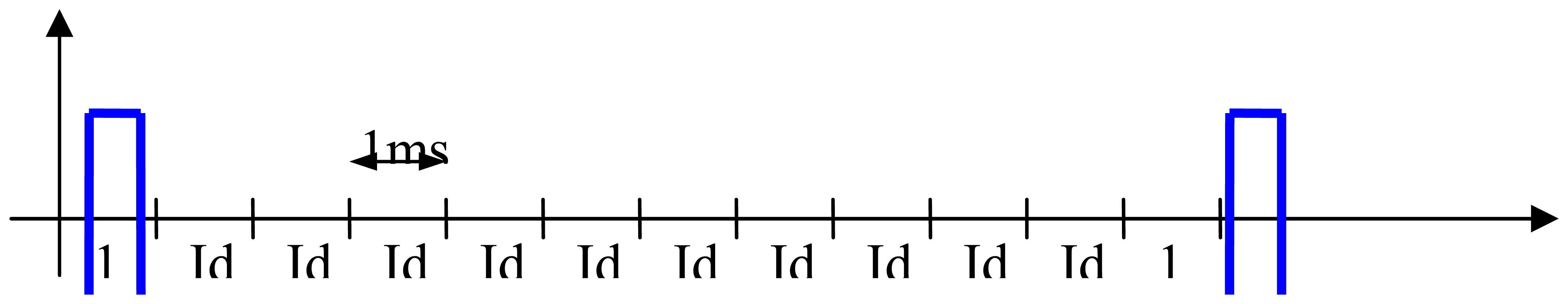
The message sent by the transmitter consists of a bit of 1 value followed by the 10 bits of the transmitter's identifier code and a final bit, also of 1 value. As can be seen in
figure 19, the time of one bit is 1ms and the transmitter understands from “1” a pulse in the transducer and from “0” the absence of signal.
Of all the possible values of the transmitter's identifier code there are two which are especially useful for studying the system-they are the identifier codes 0 and 0×3ff. The first of these can be seen as the pulse response of the whole system which is considered to cover of the transmitter, the air, the receiver and the amplifier. This is due to the fact that the message with an identifier code equal to zero only emits two “1”s separated by 10ms, a time which is much greater than the maximum damping time as will be seen later. The second one is used to detect the inter symbolic interference caused by reflections of the walls. Please see Part 5 for a better description of the measurement scenario.
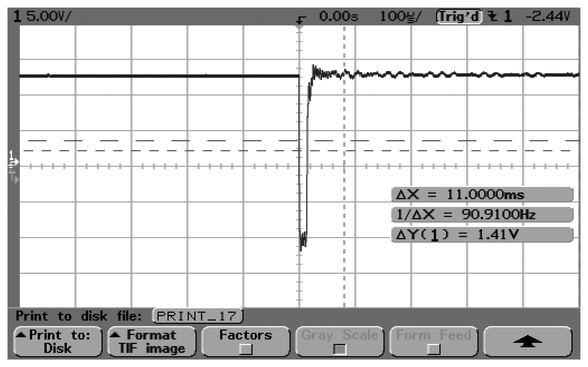
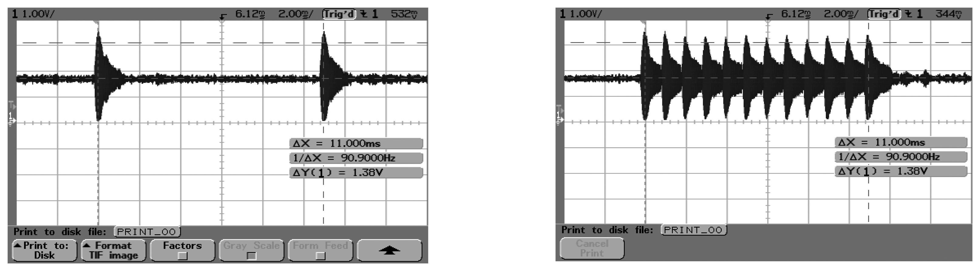
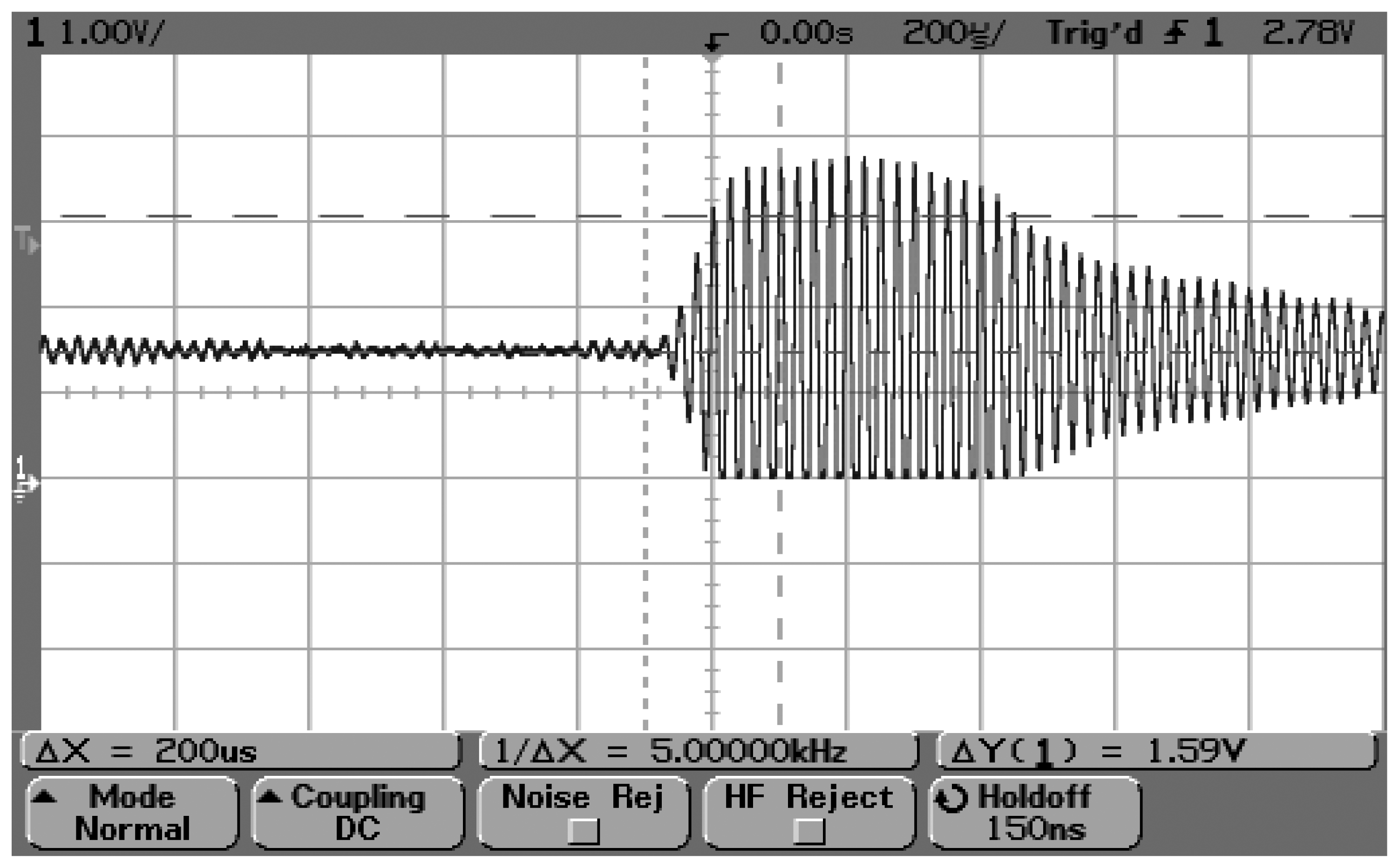
Figure 20 (a and b) shows the oscilloscope picture resulting from the receipt of a message with identity code “0” and one with identity code “1”. In both cases the receiver was vertical to the transmitter which was 4 metres above it.
Note that the answer to the impulse, that is the bit of “1” at the beginning of the message, gives a width of almost one millisecond for just one pulse of the transmitter (see
figure 21). It should be remembered that the ultrasound transducers consist of a system of damped spring mass and that this waveform results from the sum of responses to the pulses of both the transmitter and the receiver. Clearly it is no accident that the duration of a bit of the message is the same as the duration of a impulse response. Before defining the time of the bit, exhaustive tests were carried out of different types of excitation of the transmitter to determine the shortest message time without compromising the legibility of the message.
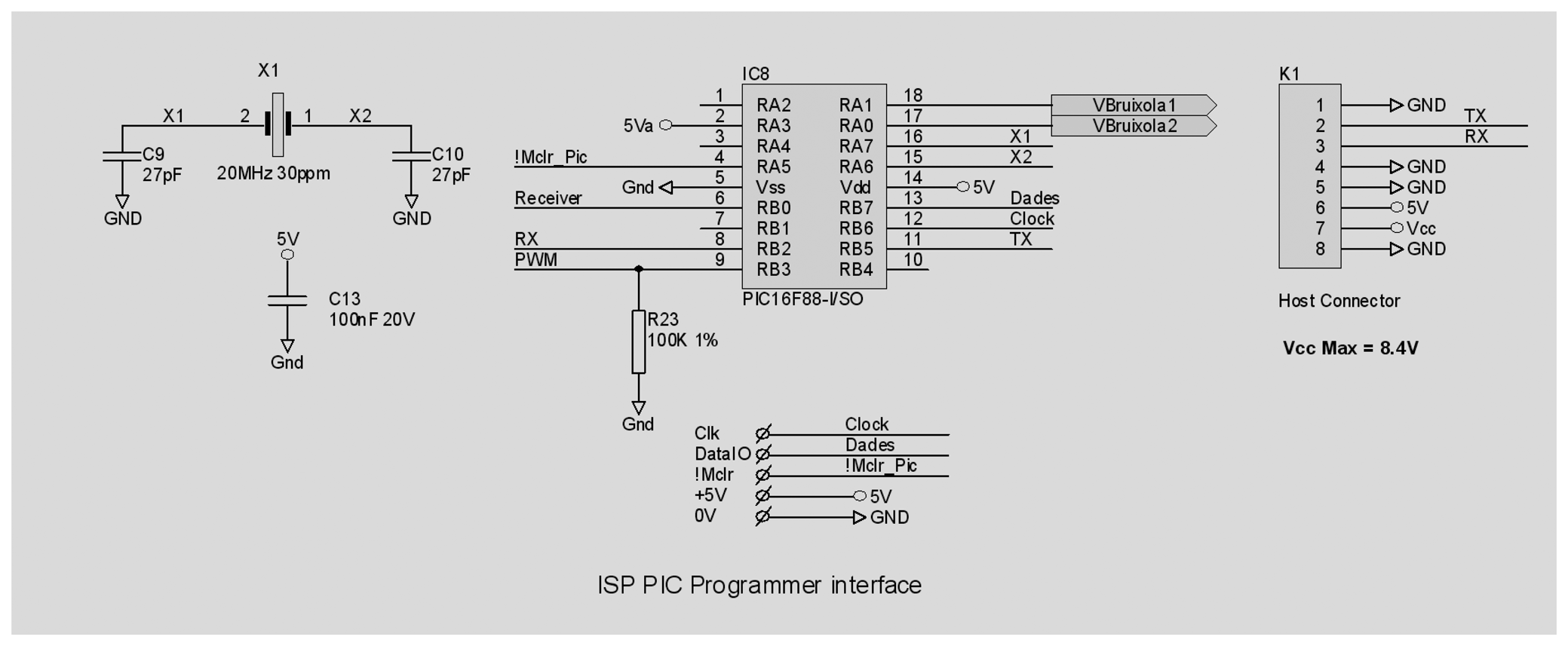
4.2 Control unit
The control unit is responsible for detecting the start of the message, calculating the delay in relation to the internal clock and for sending the identifier codes detected and the relative time between them (see
figure 22).
The heart of this unit is a microcontroller, Microchip Model PIC16F8, with a high accuracy external clock with reduced deviation to avoid adding further sources of error to those already identified. The microcontroller generates a PWM signal which allows it to vary the detection threshold level of the message according to the strength of the signal received. This signal, after passing through the IC7 comparator, is connected to the RB0 interrupt input to calculate the delay. Connector K1 connects the receiver to the host which effects the trigonometric calculations, the changes in coordinates systems and the error compensations algorithms [
8][
9] which, for reasons of space, are not described in this paper.
The data sent to the host once a second are, in addition to the identity codes and their relative delays, the direction detected by the magnetic compass and the calibration values of the compass stored in the EEPROM of the microcontroller.
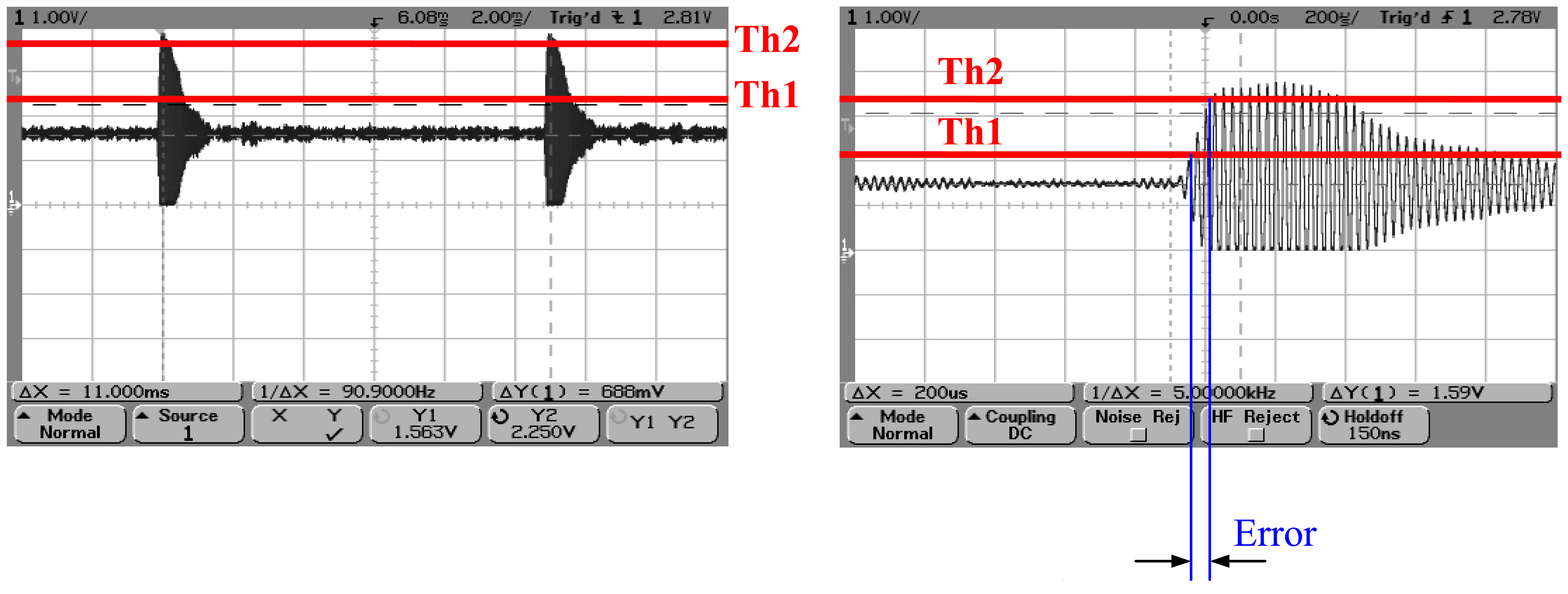
The moment when the micro-controller detects the first bit of the message depends on the threshold level set at the time and the strength of the signal received. This difference, shown in
figures 23 for two threshold levels (th1 and th2) is the third source of significant error which is referred to as “Message detection threshold error”. In order to minimize this error, processing techniques to cancel bouncing interference have been applied [
7].
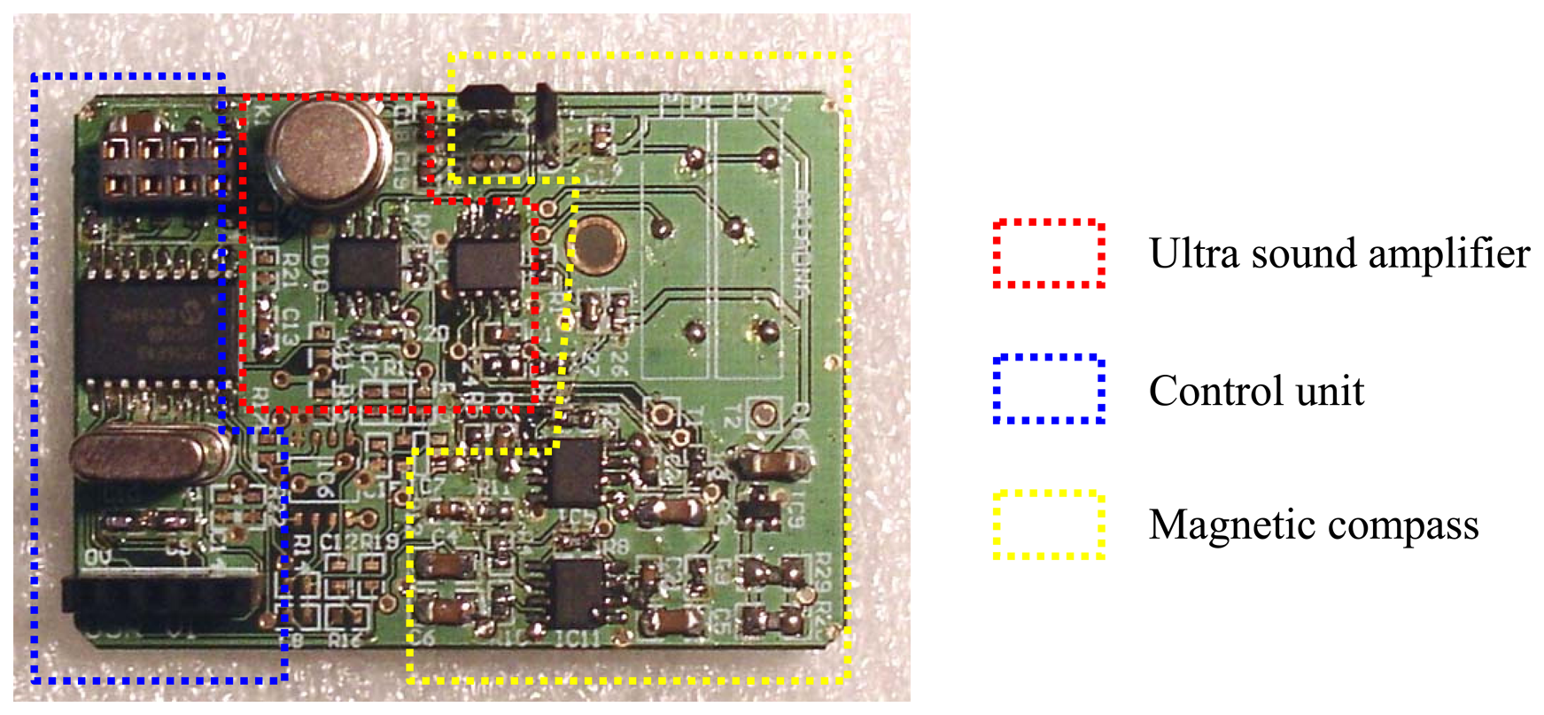
Finally, the description of the ultrasound receiver is completed with a photograph of the PCB layout in
figure 24. The receiver is 56 mm wide and 40 mm high. The 400ER80 transducer is sealed and water resistant as long as the sealing material does what it is supposed to do.
5. The Trial Scenario
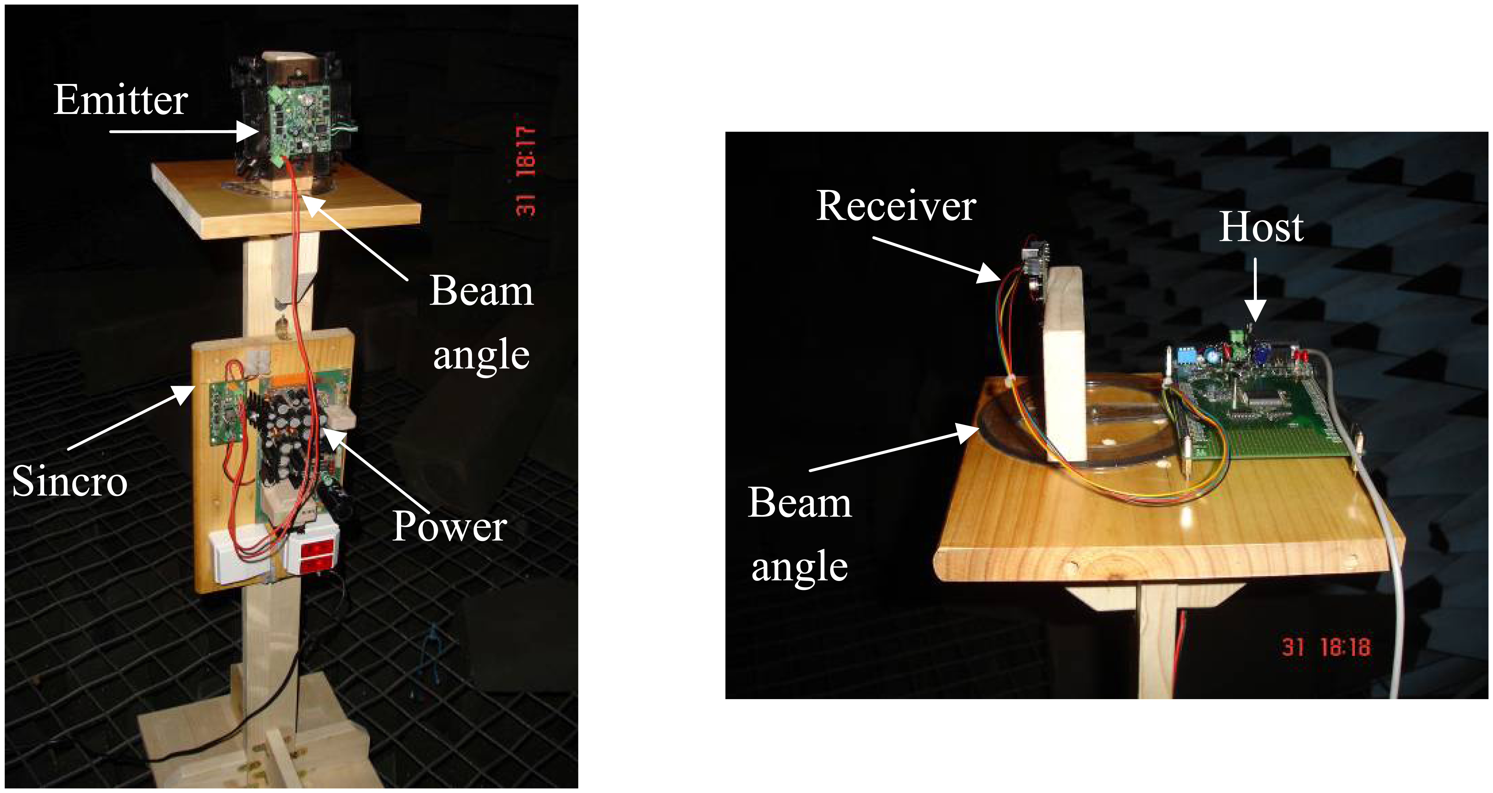
In order to test the characteristics of the various types of ultrasound transducers available in the market, 2 revolving supports were placed in the anechoic chamber of the ETSEEI of the La Salle School of Engineering and Architecture (see
figure 25).
On the left –hand side of
figure 25 can be seen the support for the ultrasonic transmitter, the power source and the clock generator necessary for activating the transmitter. On the right-hand side the ultrasound receiver connected to the host, which carries out the error correcting algorithms [
12], was set up. Using this test bed almost 20 pairs of different transducers from various manufacturers was tested to ensure their specifications coincided with reality. Once the transmitter and receiver had been chosen, the beam of reception of both of them was tested to ensure there was no blind spot in the radius.
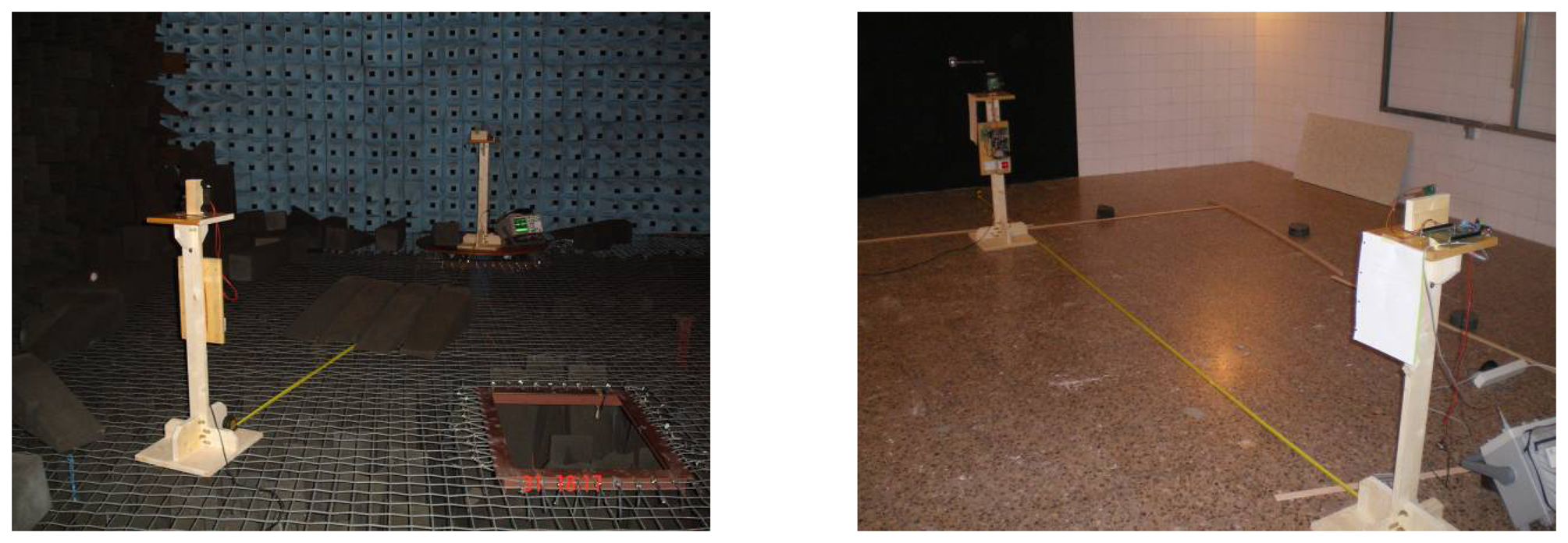
The anechoic chamber is shown in the left-hand of
figure 26 as well the beam angle test setup- in front term, the emitter, and at the end of the room the receiver and oscilloscope can be seen. The reverberation chamber is shown on the right-hand side of
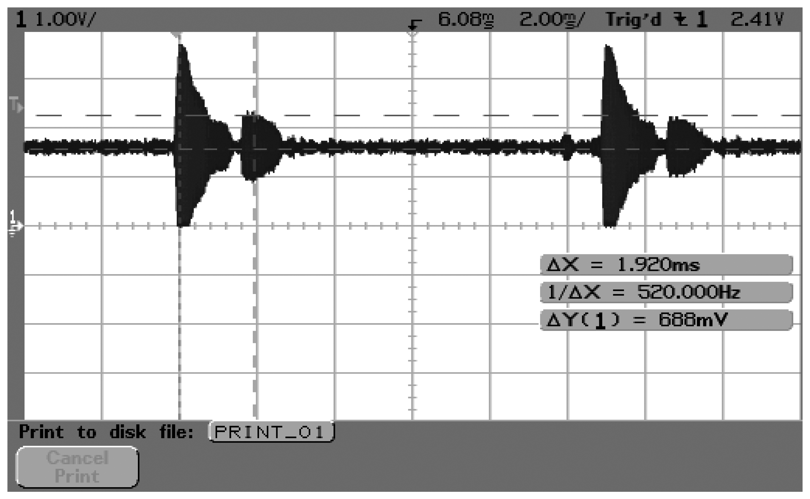
figure 26. Here the trials of intersymbolic interference caused by reflections were carried out. It was discovered that the reduction in the sensitivity of the transducer beyond 45 degrees prevents the reflections from the walls from influencing the arrival of the wave unless the wall is less than 1.5 metres from the transmitter's vertical. This needs to be taken into account in the final algorithms. In the background of the photograph can be seen the absorbent panels placed on the floor and the side wall of the chamber to make the test conditions meet our requirements. In these conditions in
figure 27 can be seen the direct message and the delayed reflection.
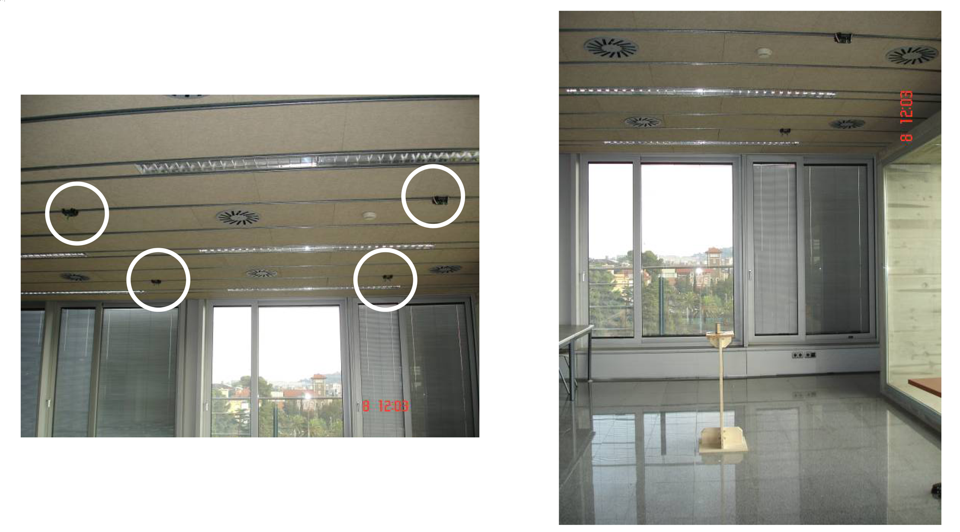
In order to evaluate the error correction algorithms a diaphanous [
4] room was used in which four transmitters were installed in the ceiling and a receiver, at a constant height, moved around the floor. In
figure 28 can be seen the four sensors installed at a fixed height and the mobile receiver setup in the floor.
The work area includes the square formed by the four emitters (enclosed by a white circle at the ceiling) but also the area near the walls, in this case the glass windows, in order to test the intersymbolic interference rejecting algorithm referenced before. Clearly this room was far from the real environment where it will be necessary to deal with shelves, air-conditioning currents, temperature variations and much more.
6. Final Considerations
The current state of this research is focused on improving the algorithms to minimise the effects of the three most important sources of error, that is, “Error in the start-up phase”, “Capacity variation error” and “Message detection threshold error”. At this time this is being carried out in the diaphanous environment described in the previous section. With temperature variations of plus or minus two degrees, the accuracy of the system is 30 cm. The next step should be a field experiment in the real environment i.e. in a supermarket and the refinement of the algorithms in situ as long as the different parameters can be maintained within reasonable limits.
Finally it should be emphasised that patent protection for this system has been applied for.
