Effect of Estimated Daily Global Solar Radiation Data on the Results of Crop Growth Models

Abstract

The results of previous studies have suggested that estimated daily global radiation (R_G) values contain an error that could compromise the precision of subsequent crop model applications. The following study presents a detailed site and spatial analysis of the R_G error propagation in CERES and WOFOST crop growth models in Central European climate conditions. The research was conducted i) at the eight individual sites in Austria and the Czech Republic where measured daily R_G values were available as a reference, with seven methods for R_G estimation being tested, and ii) for the agricultural areas of the Czech Republic using daily data from 52 weather stations, with five R_G estimation methods. In the latter case the R_G values estimated from the hours of sunshine using the Ångström-Prescott formula were used as the standard method because of the lack of measured R_G data. At the site level we found that even the use of methods based on hours of sunshine, which showed the lowest bias in R_G estimates, led to a significant distortion of the key crop model outputs. When the Ångström-Prescott method was used to estimate R_G, for example, deviations greater than ±10 per cent in winter wheat and spring barley yields were noted in 5 to 6 per cent of cases. The precision of the yield estimates and other crop model outputs was lower when R_G estimates based on the diurnal temperature range and cloud cover were used (mean bias error 2.0 to 4.1 per cent). The methods for estimating R_G from the diurnal temperature range produced a wheat yield bias of more than 25 per cent in 12 to 16 per cent of the seasons. Such uncertainty in the crop model outputs makes the reliability of any seasonal yield forecasts or climate change impact assessments questionable if they are based on this type of data. The spatial assessment of the R_G data uncertainty propagation over the winter wheat yields also revealed significant differences within the study area. We found that R_G estimates based on diurnal temperature range or its combination with daily total precipitation produced a bias of to 30 per cent in the mean winter wheat grain yields in some regions compared with simulations in which R_G values had been estimated using the Ångström-Prescott formula. In contrast to the results at the individual sites, the methods based on the diurnal temperature range in combination with daily precipitation totals showed significantly poorer performance than the methods based on the diurnal temperature range only. This was due to the marked increase in the bias in R_G estimates with altitude, longitude or latitude of given region. These findings in our view should act as an incentive for further research to develop more precise and generally applicable methods for estimating daily R_G based more on the underlying physical principles and/or the remote sensing approach.

1. Introduction

Crop growth models, which have been developed since the 1960s, have been regarded as important tools of interdisciplinary research [1] and have since been used in a number of areas such as the assessment of agriculture potential of a given region [2], in the field of crop yield forecasting [3-4] or as a climate change impact assessment tool [5-7]. In such applications lack of long-term daily weather data and especially data on global solar radiation (R_G) has often been a significant challenge, since R_G is an indispensable input variable for the majority of these models that simulate crop growth, because photosynthesis itself is primarily driven by solar radiation. Moreover, global solar radiation is a key input variable for methods used at present for potential and actual evapotranspiration estimation, which is an essential part of water balance subroutines in almost all crop models. Other types of mathematical models for crop growth and development (apart from the process-oriented methods) rely frequently on R_G as one of the key independent variables [8-9] and their outputs might be clearly affected by any R_G bias. It has been noted many times [10-12] that continuous records of global solar radiation measurements are spatially scarce and that the ratio between the number of stations observing daily R_G and those measuring temperature and precipitation is highly variable from less than 1:10 in Germany [13] or 1:20 in the Czech Republic [14] to 1:500 on the global level [15]. The spatial density of weather stations providing complete climatic data sets for crop model inputs is therefore inadequate and the missing R_G data have to be substituted. Missing daily radiation data at a given site can either be substituted by data measured at a nearby station [12, 16-18], estimated by remote sensing techniques [19-20], or produced by some other method. These methods include stochastic weather generators [21-23], linear interpolation [24], use of higher order statistics [25], application of the neural network method [26-27], or the application of various empirical or semi-empirical relationships established between daily global radiation and other more frequently measured meteorological parameters [28-30].

Published studies conducted under European conditions suggest relatively small threshold distances (depending on topography and other factors) for substituting R_G data from a nearby station [14, 16] compared with other regions [17]. Stochastically generated data may be useful for exploring possible model scenarios for an average theoretical situation using long-term simulations, but they cannot be used for model validation and simulation analysis during a particular period of time [11]. It should also be remembered that the weather generator use would require a time series of observed data (several years at least) in order to set statistical parameters for a particular site. Widespread application of the other two mentioned methods, i.e. linear interpolation and use of neural network analysis in crop growth modelling, is limited for the same reasons as in the weather generator approach and in some cases yield worse results than empirical models [26]. Despite dramatic developments in remote sensing techniques that have made vast databases of R_G data available on an unprecedented scale to users, empirical models estimating R_G from commonly measured meteorological variables remain an important tool in many agrometeorological applications. Numerous formulas have been made available in previous decades, which might make selection of the most appropriate method for a particular purpose and site. Some of these methods have already been incorporated into crop models as an integral part of the software package, like in case of STICS [31] or SWAP models [32]. Others are developed as standalone applications [33] for use in crop model studies in order to facilitate the preparation of the necessary weather data.

Despite over 40 years of crop model development, the effect of this type of uncertainty on simulated crop parameters has not yet been fully researched or else it is considered to be of minor importance compared with other sources of bias [34-35]. It has often been reasoned in literature that the overall effects of biases in R_G data will cancel each other out over the growing season [17, 34, 36] and can thus be neglected owing to uncertainties in other parameters. This claim is based on the following assumptions: i) R_G biases are more or less normally distributed with a mean of zero; ii) the relationships between R_G value biases and yield estimates are more or less linear; and iii) any error in yield estimates introduced by systematic or random error in R_G data is insignificant compared with the overall yield. However, as Nonhebel [16] noted, the error in R_G data is unlikely to cancel out simply because of the complexity of the crop model response. Moreover, the mean biases of the substitute R_G data are frequently different from zero and R_G data based on some of the frequently used estimation methods are loaded with significant bias [14, 37].

Up to now only limited efforts have been made in the area of “indirect” evaluation of the methods for R_G estimates, i.e. by comparing crop model outputs attained using observed R_G inputs with estimated ones [18,24,36,38]. Most of these studies dealing with crop model sensitivity to R_G have evaluated only the effect of the constant deviation in R_G values during the growing season [17,39]. It is questionable whether such approach reflects the real distribution of systematic and random errors over the season for the particular R_G estimation method and whether this approach can be used to predict crop model biases. In order to explore the effect of these uncertainties, seven R_G estimations were chosen and their performance in crop models compared using data from eight Austrian and Czech stations representative of the Central Europe lowlands. The methods were selected on the basis of: 1) general availability of required input data; 2) practical applicability, which was judged mainly by availability of the necessary empirical coefficients; and finally 3) their previous/planned application in crop model studies in the study area.

Another field where the uncertainty in the R_G inputs is particularly troubling is the spatial analysis of crop growth using crop models over larger regions. Whilst sufficient station density is available for most weather data inputs, there is a general shortage of sites with observed global radiation data. Moreover, not all of these sites could be used because of their location within urban areas or at high altitudes. On average, we found that there is less than one station per 8000 km² (after discarding non-suitable stations) in Central Europe. Therefore any spatial application of the crop model in this region (and in other regions as well) has to use some form of estimated R_G data [40-43]. In the Czech Republic the most obvious choice is to use hours of sunshine, but the Campbell-Stockes heliographs used for measurement make online reporting of the results impossible at most of the stations and these data are available only with a time lag of several weeks. In addition, there are concerns about the homogeneity of observed sunshine duration series obtained by different instruments that can lead to a significant bias in R_G estimates. For example, during the 1980s and 1990s the widely used Campbell-Stokes sunshine duration autographs were replaced in several countries by optoelectronic sensors such as the HAENNI SOLAR 111B. Differences between these two measurement systems observed in Austria have been reported to the WMO [44] and were found to be of the order of 5 per cent or more [45].

All of this poses a problem for some crop model applications (e.g. crop growth monitoring) requiring input parameters to be available in near real time [10]. The second part of the study is thus focused on testing the uncertainty in regional crop model outputs assuming two likely scenarios assuming availability of 1) daily extreme temperatures and total precipitation data; and 2) only daily extreme temperatures. The methods based on cloud cover were not considered in this part of the study as these data were not available in our database for a sufficient number of stations and because with the increasing number of automated weather stations this parameter is not measured. The overall objective was to quantify the uncertainty arising from the use of various R_G methods and to compare it with the results found at the local level. The list of the selected methods is not fully representative, as numerous alternatives exist. The authors tried to include a range of methods using readily available input variables to provide a notion of effectiveness of individual predictors. In the presented analysis, the empirical coefficients for all methods were based on literature sources. We are aware that this procedure might lead to much larger deviations than those referred to in recently published studies, which in general operate with key equations parameterized with the help of solar radiation data measured at the given site. However our approach, i.e. using literature-based coefficients, is more realistic as in number of cases R_G values are simply not available. Similar approximations are also necessary when the spatial assessment of crop growth and development is performed.

2. Material and Methods

We hypothesized that the non-linearity in the crop model algorithms could result in amplification or attenuation of input data inaccuracies, which could seriously distort the overall model performance. In order to test the initial hypothesis, the following steps were undertaken: (i) Assessment of the crop model output sensitivity to the various R_G estimation methods using detailed crop models at selected sites; (ii) R_G error propagation and consequences for nationwide crop modeling systems (used for climate change impact studies or for the yield monitoring, for example); (iii) Discussion of the consequences of crop model inaccuracies caused by R_G data and strategies for their limitation.

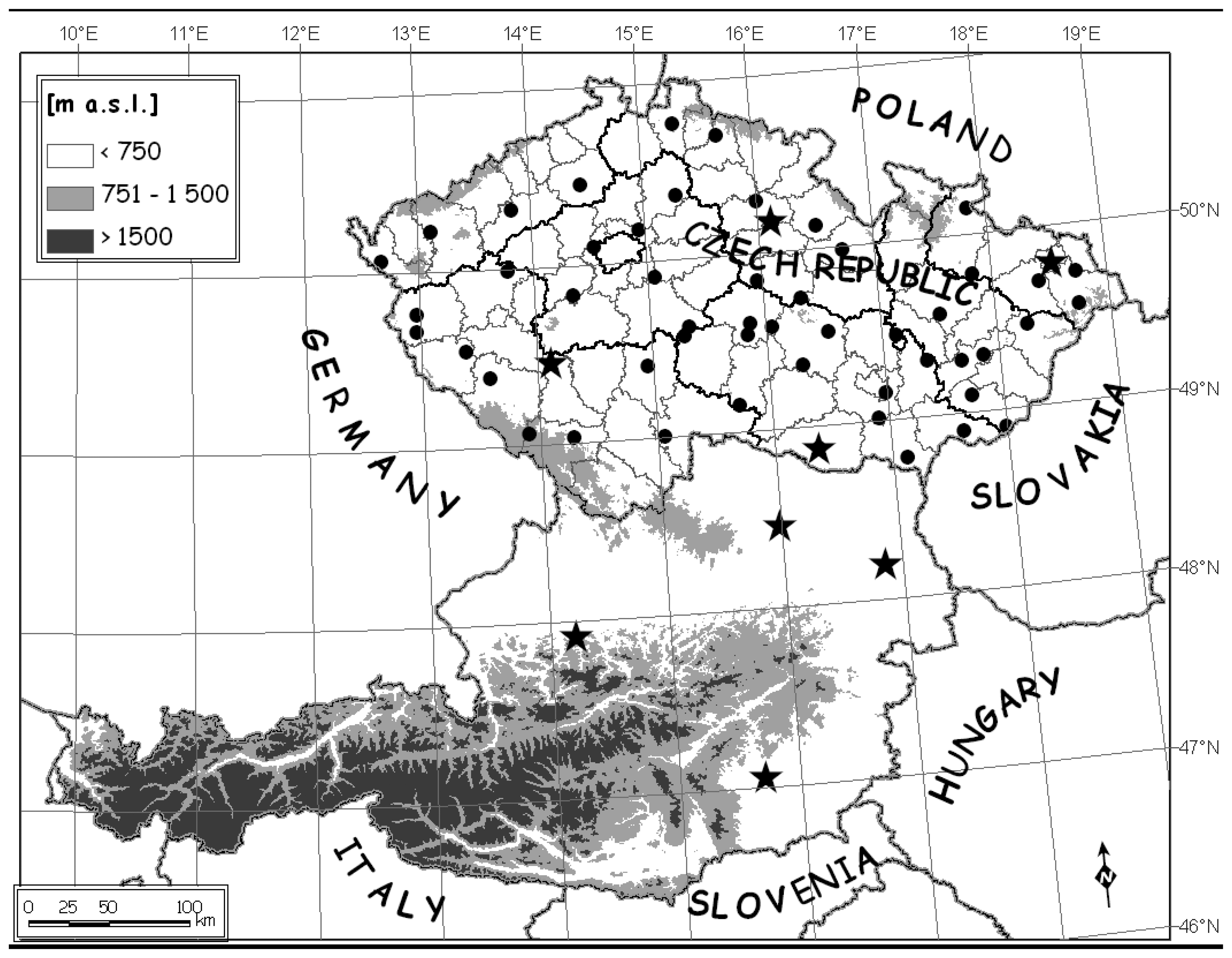
2.1. Definition of the Study Area

The overall climate of the study area (Fig. 1) is influenced by the mutual penetration and mingling of the ocean and continental effects. It is characterized by prevailing westerly and north-westerly winds, intensive cyclonal activity causing frequent alterations of air masses and comparatively high precipitation. The altitude and geographical relief influence the climate, especially in Austria where the orographical impact of the Alps must be taken into account. However, both parts of the study were aimed at performance of cereal crop models in intensively cultivated regions (generally less than 750 metres above sea level). Area below this threshold accounts for 50 per cent in Austria with most of arable crop production concentrated there. The topography of the Czech Republic is rather different: more than 92 per cent of the land is below 750 metres above sea level, which means that over 54 per cent of total area can be cultivated, with 72 per cent of arable land. Spring barley and winter wheat are among the top six crops in both countries and they account for the largest portion of the cereal production in both countries. The first part of the study was based on detailed datasets collected at eight sites with continuous R_G measurements, which were obtained from the databases of the Austrian Meteorological Service (ZAMG) and Czech Hydrometeorological Institute (CHMI). These sites have high quality, homogeneous daily records for six years or more of T_min, T_max and T_avg, precipitation, cloud cover, total daily sunshine and global solar radiation. Data from 16 stations were originally considered and after careful verification of the completeness and homogeneity of data, the final list of eight stations was selected for this study with 97 years of complete daily data. No long-term trend in the observed R_G data [e.g. 46] was taken into account, because the data series are relatively short and in most cases not continuous for such trends to be evaluated. Daily total extraterrestrial radiation (R_A) was calculated as a function of latitude, day of the year, solar angle and solar constant according the procedure suggested by [47] and details are given in [14].

The second part of the study focused on uncertainties in the spatial yield assessment and monitoring using estimated R_G values of varying precision. Analysis was performed only on the territory of the Czech Republic since the digital soil map of Austria was not available to the authors. Daily weather conditions of the Czech Republic were represented by the set of 52 stations with observed data on daily hours of sunshine, T_min, T_max, precipitation, mean wind speed and water vapour pressure available for the period 1961-2000. Out of the total number, 45 could be considered as non-urban stations that are not significantly affected by large agglomerations while the remaining stations are located on the edge of urban areas. In all cases station location and measurement procedures follow WMO standards. The spatial distribution of these stations is shown in the Fig. 1 and most of them are situated below 750 m, which is regarded as the upper boundary for cereal production. The lowest station is 171 m above sea level (with a mean annual temperature 9.3°C and total precipitation from 1961 to 1990 of 481 mm) whilst the station with highest altitude is at 1324 m (with a mean annual temperature of 2.6°C and 1391 mm total precipitation). The mean altitude of the selected station is 448 m, which is close to the country mean altitude (430 m) with overall mean annual temperature and precipitation totals that are almost identical with the mean climatological values of the Czech Republic i.e. 7.5°C and 674 mm respectively.

2.2. Methods of Estimating Daily R_G Values

The site-specific R_G estimates were based on four groups of methods with different weather parameters from which the daily R_G value is estimated i.e. (i) sunshine duration, (ii) cloud cover and temperature, (iii) temperature and total daily precipitation, and (iv) temperature data alone. The calibration of the methods was not considered in the study despite the fact that the precision of some of the methods could probably have been increased in that way. As mentioned earlier, the empirical coefficients necessary for individual methods were based on literature sources, which on the one hand leads to larger errors in the estimates but which realistically represents the challenge that most modellers have to deal with. In our experience estimated R_G data are used in most crop modelling studies because of the lack of measured R_G data at the site, which makes it difficult to calibrate a particular R_G method. A detailed description and performance analysis of seven methods used for R_G estimation can be found in the preceding study [14] and in other related works listed below. The overview of the performance of individual methods is presented in the Annex I.

The Ångström formula [28] improved by Prescott [48] is the most common choice in crop model studies at sites where no R_G measurements are available. It is based on the fraction of daily total atmospheric transmittance of the extraterrestrial solar radiation (R_A), which is determined as a fraction of actual (n) and potential sunshine duration (N) during the day:

$$R_G=R_A\left(a_A+b_A\frac{n}{N}\right)$$

(1)

where a_A and b_A are empirical coefficients determined for the particular site. The Ångström-Prescott coefficients were interpolated using maps available at http://www.treemail.nl/privateers/radiation/index.htm (2007), which were originally developed within the MARS project. This method will be referred to as Eq. (1).

The second method (Eq. (2)) is based on the statistical analysis of the relationship between the measured R_G and the relative sunshine duration. The equation is based on the observed R_G in the Hradec Králové solar observatory (Fig. 1) from 1960 to 1979 and was developed by Klabzuba et al. [29] in the following form:

$$R_G=7.19+0.258\frac{\text{n}}{\text{N}}-{\mathrm{9.28.10}}^{-6}\left(\frac{\text{n}}{\text{N}}+22.9\right){\left(JD-174.7\right)}^2$$

(2)

where JD stands for the Julian day number. The method was intended for use in applications such as crop growth models and climate models for the Czech Republic and the main advantage is its simplicity. On the other hand as it was derived for a single location in the Czech Republic and by definition it should be used only within similar climatic and orographical conditions for which it was developed i.e. in the Central Europe north of Alps.

One of the most important atmospheric phenomena limiting solar radiation at the Earth's surface are clouds and accompanying weather patterns [10]. In this study the following combination of Wörner [49] and Hargreaves et al. [50] models proposed by Supit and van Kappel [10] was applied and is referred to as Eq. (3):

$$R_G=R_A\left[a_S\sqrt{\left(T_{max}-T_{min}\right)}+b_S\sqrt{\left(1-C_W\right)\frac{1}{8}}\right]+c_S$$

(3)

where C_w is the mean total cloud cover during daytime observations (octa), T_max and T_min stand for the maximum and minimum daily temperatures and a_S, b_S and c_S symbols are assigned to empirical constants that are available at http://www.treemail.nl/privateers/radiation/index.htm (2007).

Most of methods applying diurnal temperature range and daily total precipitation were designed because of the general availability of these inputs from weather stations [11, 36]. The method proposed by Winslow et al. [30] and referred to as Eq. (4) was designed as a globally applicable model. The prediction equation is:

$$R_G={\tau }_{cf}D\left[1-\frac{\beta e_s\left(T_{min}\right)}{e_s\left(T_{max}\right)}\right]R_A$$

(4)

where e_S(T_min) and e_S(T_max) are saturation vapour pressures at temperature T_min and T_max, respectively. Variable τ_cf accounts for atmospheric transmittance and is estimated from site latitude, elevation and mean annual temperature. Function D corrects for errors introduced by site differences in day length. This error arises from the difference between the time T_max at which relative humidity reaches its minimum and sunset at which R_G reaches its total daily value. The value β is a coefficient that remains stable in lowland areas and a value of 1.041 was therefore used as recommended by [30].

The method proposed by Thornton and Running, [51] is based on the Bristow and Campbell [52] study and is as follows:

$$R_G=R_A\times T_{t,max}\times T_{fmax}$$

(5)

where T_t,max is the maximum (cloud-free) daily total transmittance at a location with a given elevation and depends on the near-surface water-vapour pressure on a given day of the year, and T_{f max} stands for the proportion of T_t,max realised on a given day (cloud correction). The modified version of the method including the snow pack model was included in the present study as Eq. (5) because this particular modification improves the estimated R_G precision during winter months. The radiation algorithm parameters were set according to the results, which were derived for the conditions in Austria and are generally applicable throughout Central Europe (Thornton, 2003, personal communication).

Using only daily extremes of air temperatures to estimate atmospheric transmissivity provides a strong physical basis that in combination with good data availability makes such methods very popular [11,50,53,54]. The approach was exploited further by Donatelli and Campbell [54] with the following result (Eq. (6)):

$$R_G=R_A\tau \left[1-exp\left(-bf\left(T_{\mathit{\text{avg}}}\right)\mathrm{\Delta }{T}_i^{2}f\left(T_{min}\right)\right)\right]$$

(6)

where τ stands for the clear sky transmissivity (set to be 0.75), ΔT, f (T_avg) and f(T_min) are functions based on the daily mean and minimum temperatures and b is an empirical parameter, which can be parameterised for a given site using readily available climatological data, e.g. mean June temperature and mean annual temperature (excluding June).

Another relatively simple method of estimating daily global radiation by relating the daily temperature range (the difference between maximum and minimum temperatures) to global radiation was proposed by Hargreaves et al. [50]:

$$R_G=R_A{a}_H\sqrt{\left(T_{max}-T_{min}\right)}+c_H$$

(7)

where a_H and b_H are the empirical constants derived from maps published at www.supit.net (2007). However, owing to the lower accuracy of the model, its application for locations in Europe is considered to be limited [55]. This method is numbered Eq. (7) in the study.

The overall performance of all methods at the eight experimental sites is described in

Table 1. Summary of performance of various methods of R_G using regression coefficients, annual mean bias error (MBE) and annual root mean square error (RMSE). The results are based on the pooled data from the 8 observational sites with total 97 complete years of record.

Parameter	Eq. (1)	Eq. (2)	Eq. (3)	Eq. (4)	Eq. (5)	Eq. (6)	Eq. (7)
	Ångström-Prescott	Klabzuba et al.,	Supit and van Kappel,	Winslow et al.	Thornton and Running	Donatelli and Campbell	Hargreaves et al.
	[28,48]	[29]	[10]	[30]	[51]	[54]	[50]
YEAR
a)R2	0.96	0.94	0.91	0.86	0.82	0.82	0.83
b)Sl	0.99	1.03	0.99	0.97	0.92	0.99	0.99
c)MBE	1.1	5.20	1.7	1.70	3.00	2.90	6.32
d)RMSE	14.50	20.39	24.71	28.60	29.74	32.03	32.05
SPRING BARLEY GROWING SEASON (IV-VII)
R2	0.90	0.91	0.77	0.67	0.62	0.61	0.61
Sl	1.00	0.99	0.99	1.01	0.99	1.03	1.02
MBE	0.1	0.4	2.0	6.0	2.5	8.1	9.6
RMSE	11.4	12.6	17.2	23.1	23.5	26.5	26.5
WINTER WHEAT GROWING SEASON (X-VII)
R2	0.97	0.94	0.91	0.87	0.85	0.85	0.84
Sl	0.99	1.02	0.99	1.01	0.99	1.02	1.01
MBE	1.3	3.4	1.4	3.6	6.3	4.0	8.1
RMSE	15.0	20.1	23.9	30.0	32.1	33.6	33.7

Note:

^a)Values of coefficients of determination of the linear regression line with the best fit.

^b)Values of slope of the regression line forced through the origin.

^c)Relative value of the annual mean bias error expressed in %.

^d)Relative value of the annual root mean square error expressed in %

both for the whole year and for the growing season of two model crops i.e. spring barley and winter wheat. The Eq. (1), was found to be the best of the tested methods (Table 1). It explained 96 per cent of the R_G variability with very low systematic bias. If there are no reliable sunshine duration data available at the site, the Eq. (3), yields the most precise estimates. If neither cloud cover nor sunshine duration data are available, the Eq. (4), which employs the daily precipitation total, might be used for the winter wheat growing season whilst the Eq. (5) seems to perform better for the months of the spring barley growing period. If only T_max and T_min are measured at the site, then Eq. (6) shows lower bias than the Eq. (7).

2.3. Crop Models

The impact of uncertainties in the daily R_G estimates on crop model outputs was assessed with the help of two crop-environment resource synthesis (CERES) models (namely CERES-Barley [56] and CERES-Wheat [57]) together with the WOrld FOod STudies [58, 59] model. Both CERES models were used for detailed site-specific analysis of inaccuracies caused by estimated R_G values at eight selected sites, as they allow a detailed insight into the key processes of crop growth. On the other hand the design of the WOFOST model and limited data requirements have made it the prime choice for spatial yield assessment or crop monitoring [60] or climate change impact assessments [61, 62]. In both the CERES and WOFOST models the temperature is the driving force behind the phenological development and modifies daily gross photosynthesis and controls respiration processes. The CERES model calculates dry matter accumulation as a linear function based on intercepted photosynthetically active radiation and radiation use efficiency [63]. The photosynthetically active radiation is assumed to be half the input daily solar radiation, thus making the daily R_G total one of the key driving variables. The fraction of PAR intercepted by the crop canopy then depends on the extinction coefficient and leaf area index on the given day and thus the final relationship between the R_G and dry matter yield does not strictly follow linear trends.

Another source of nonlinearity in the R_G vs. simulated biomass production relationship is the method of deriving daily actual dry matter accumulation. It is a product of the potential daily dry matter accumulation (based on the amount of biomass already present from previous days and the actual leaf area index) and correction factors accounting for the water and/or nitrogen stress (which are partially R_G dependent) and non-optimal temperature. When the grains begin to grow they become the dominant sink for the storage of assimilates and have priority for all above-ground assimilate production, thus again changing the pattern of the R_G uncertainty impacts. CERES models also account for the mobilisation and redistribution of mobile reserves, which were stored in the stem during days when the biomass production is inadequate for sink-controlled grain growth. More details on the processes involved can be found in [57, 64, 65] and also in the overview paper by Jones et al. [66].

WOFOST uses a detailed approach to describe the light interception of the canopy with account taken of site-specific atmospheric transmissivity, incoming diffuse and direct light, reflection and scattering within the canopy as well as light absorption [59]. Daily gross assimilation increases non-linearly with both increasing irradiation and LAI. As in the case of CERES model, gross assimilation is limited by the developmental stage dependent light saturation point under the potential production situation. However, the light saturation point is rarely encountered in Central European conditions. As the light interception increases non-linearly with LAI, any error in R_G estimates at a high LAI value (typically in the key developmental stages) leads to strong non-linear assimilation responses. In a water-limited production situation (which was considered in our study) R_G additionally controls the soil evaporation and plant transpiration accounted for by the Penman-Monteith equation [59]. Similar to the CERES model, overestimation of the daily R_G will lead to overestimation of the potential evapotranspiration and thus higher soil water depletion. If the soil water is not adequate to meet the demands of the crop, higher water stress reducing growth will occur and will be consequently more pronounced during dry years. In contrast to the CERES model, the WOFOST soil water balance sub-model considers the soil profile to be homogeneous, thus significantly reducing input data requirements in Central European conditions, where there is high spatial and vertical soil heterogeneity. Consequently on the site level, the WOFOST model tends to perform with lower precision at individual sites than more sophisticated models such as CERES [67]. This was the main reason for selecting different models for both types of analyses.

2.4. Setting up the CERES Models for Site Specific Simulation Runs

At each out of the eight solar radiation observatory site (Fig. 1) the CERES-Wheat and CERES-Barley models were run with the observed weather data sets composed of daily T_max and T_min temperatures, total precipitation and observed daily R_G sum. Then the observed R_G values were replaced by R_G estimates based on Eqs. (1) - (7) while other weather variables were kept the same as in the control run. In order to fully examine the effect of errors in R_G estimates under different soil conditions, three soil types were considered. The characteristics of the soil types were obtained from lysimeters at the Federal Office and Research Centre for Agriculture in Hirschstetten, Vienna, Austria. The soils represent main soil types in the centre of the study region (i.e. lowlands of Austria and Czech Republic) and can be characterised as follows i) chernozem on fine calcareous sediments, referred to here as chernozem (USDA classification scheme: silty loam); ii) chernozem on fine calcareous sediments over gravel and sand, referred to here as sandy chernozem (USDA classification scheme: sandy loam) and iii) calcaric fluvisol, referred to here as fluvisol (USDA classification scheme: silty clay loam). The basic properties of the soil types are shown in the

Table 2. Overview of measured and derived* soil parameters in the three top profiles that were used as crop model inputs: bulk density (BD), organic carbon content (OC), soil water content at the saturation point (θ_SAT), field capacity (θ_FC) and wilting point (θ_WP).

Chernozem
Depth (m)	BD (g cm-3)	OC (%)	θWP (m3 m-3)	θFC (m3 m-3)	θSAT (m3 m-3)
0.3	1.33	2.70	0.21	0.35	0.43
0.6	1.52	0.40	0.16	0.32	0.40
0.9	1.49	0.20	0.11	0.36	0.42
Sandy chernozem
0.3	1.56	1.30	0.08	0.28	0.37
0.6	1.52	0.40	0.05	0.19	0.39
0.9	1.49	0.20	0.05	0.19	0.39
Fluvisol
0.3	1.37	2.88	0.20	0.35	0.42
0.6	1.35	2.58	0.18	0.34	0.42
0.9	1.38	2.46	0.18	0.35	0.40

. The selected soil types represent the most fertile soils in the regions on which winter wheat and spring barley are grown. Key field operation input data and the definition of the initial conditions (

Table 3. Setting of the key CERES-Barley and CERES-Wheat input parameters based on the experimental data.

Soil	chernozem		sandy-chernozem		Fluvisol
	s.barley	w.wheat	s.barley	w.wheat	s.barley	w.wheat
Start of the simulation	1st January	10th October	1st January	10th October	1st January	10th October
Sowing date	22nd March	10th October	22nd March	10th October	22nd March	10th October
Sowing density (seeds.m-2)	600	600	400	400	650	400
Harvest date	16th July	9th July	16th July	9th July	16th July	9th July
Dose of N fertilizer (kg.ha-1)	50	120	50	70	50	120
Initial soil NO3 (kg.ha-1)	25.6	25.6	2.1	2.1	29.8	29.8
Initial soil NH4 (kg.ha-1)	4.2	4.2	0.4	0.4	8.4	8.4
Initial available soil water in the soil profile (mm)	370	370	206	206	321	321

) were also based on the lysimeter experiment as reported in [67]. In the present study the effect of weeds, pest and diseases on the crop was not considered. The parameters of two Czech-bred cultivars (AKCENT for spring barley and HANA for winter wheat) that are well adjusted to the local conditions [68-69] were used in the study. The cultivar specific parameters were derived in two previous independent studies that used either observed daily R_G sum or in some cases combination of observed data with locally calibrated Eq. (1).

2.5. Setting up the WOFOST Model for Spatialised Simulation Runs

In order to test the effect of estimated R_G values on the spatial estimates of winter wheat yield, five sets of solar radiation estimates were prepared for each weather station. As observed daily R_G values were available at only ten sites in the region, we selected the Eq. 1 as the reference method based on a preceding study [14]. In the next step the daily R_G values for each site were estimated using Eqs. (4)-(7). The soil conditions in the Czech Republic were characterised by the spatialised soil database containing 25 different soil types with 1×1 km grid according to [70]. The basic soil properties required by the WOFOST model (i.e. maximum rooting depth, soil water content at wilting point, field capacity and saturation, and also soil hydraulic conductivity) were based on the database of the complex soil survey of the Czech Republic that contains 1078 soil pits with details on the soil physical properties. For this particular study the soil pits were sorted according to the soil type, and mean input parameters were calculated for each of them. The initial soil water content at the beginning of the season was set at 60 per cent of the maximum retention capacity. The spatial analysis using the WOFOST model was carried out within the PERUN crop modelling system [71] using multiple site simulations. It allowed WOFOST simulations to be run for all possible combinations of 52 weather stations and 25 soil types and the 1961-2000 period. Based on these 40‐year model runs, mean as well as quartiles, maximum, minimum and standard deviation values for selected model outputs (crop yield, harvest index, water stress etc.) were calculated for each of 1300 combinations of station and soil type. Then these model outputs were interpolated to individual 1 × 1 km grids using the value of the selected parameter at the closest weather station for the particular soil type corrected by the trend function. The trend function was determined for each of the soil types using altitude, longitude and latitude of all weather stations as independent variables and simulated value of the crop parameter as a dependent one.

The subsequent analysis using ArcInfo® GIS software allowed us to display only arable land. Finally the results for individual grids were aggregated at various NUTS (Nomenclature of Units for Territorial Statistics) levels, which included districts (NUTS 4), regions (NUT 2) and the whole Czech Republic (NUTS 0). The spatial analysis focused on the assessment of the long-term productivity of each grid (i.e. mean yield for period 1961-2000; standard deviation of the grain yield and it minimum and maximum values), even though analysis of individual seasons would have been possible as well.

2.6. Evaluation of the Model Outputs

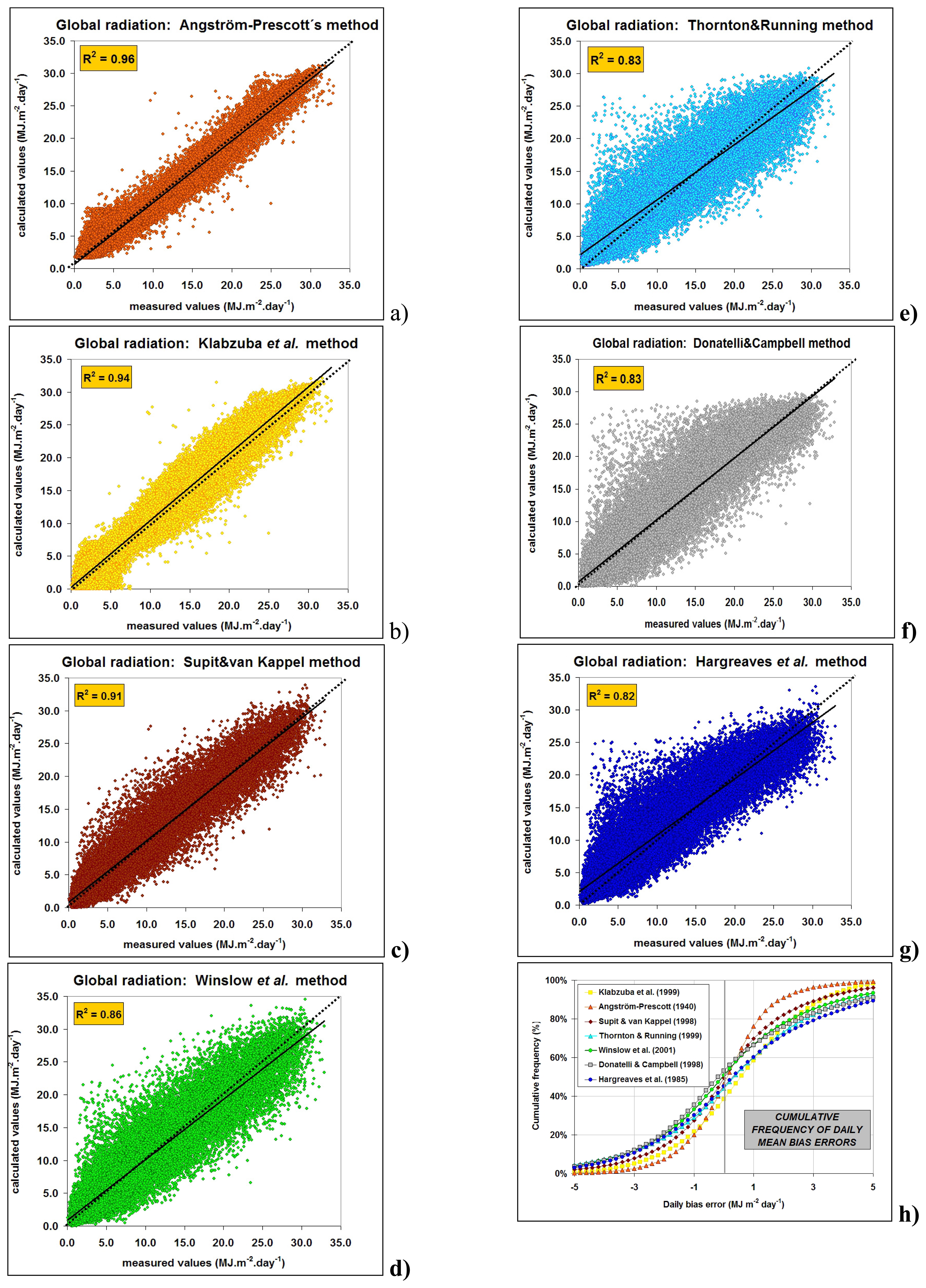
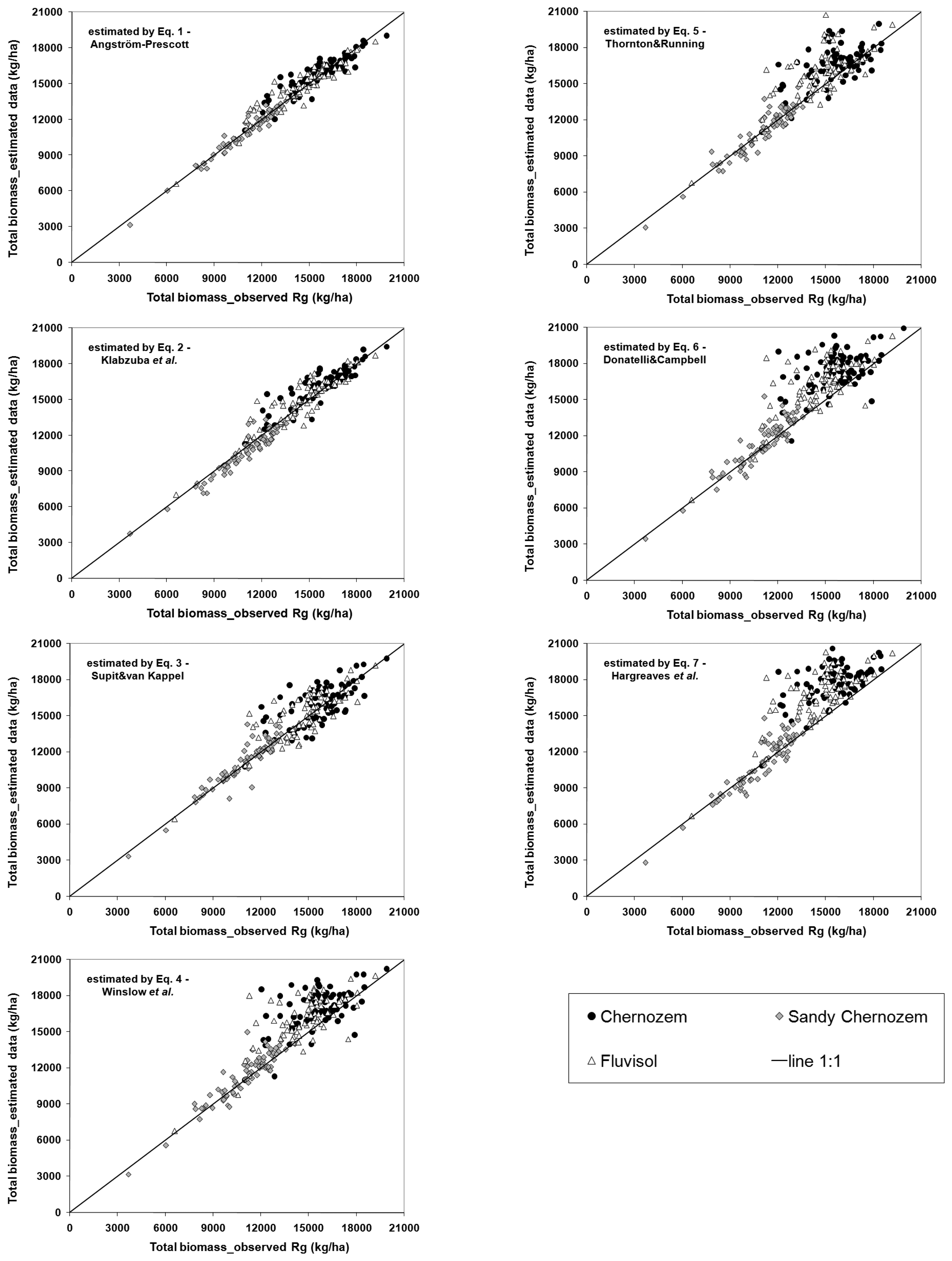
The effect of the R_G estimate method compared with the control run (based on the observed or the best available method for R_G estimate) was assessed for both crop models on the basis of four characteristics: (i) the mean bias error (MBE) as an indicator of systematic error; (ii) the root mean square error (RMSE), which can be divided into random (RMSE_r) and systematic components (RMSE_s) and thus it allows the magnitude of both systematic and non-systematic error to be assessed [72, 73]; (iii) slope of the regression line forced through zero; and (iv) the coefficient of determination of the best-fit regression line. The relative MBE and RMSE values were determined as the ratio of the appropriate characteristic and the average value for the given sequence of crop model runs.

The MBE is calculated as:

$$\mathit{\text{MBE}}=\frac{\sum (Q_{\mathit{\text{obs}}}-Q_{\mathit{\text{est}}})}{N_{\mathit{\text{obs}}}}$$

(8)

where Q_obs and Q_est are substitute crop model runs with observed and estimated global radiation values and N_obs is the number of crop model runs.

The RMSE is calculated as:

$$\mathit{\text{RMS}}E=\sqrt{\frac{\sum {(Q_{\mathit{\text{obs}}}-Q_{\mathit{\text{est}}})}^2}{N_{\mathit{\text{obs}}}}}$$

(9)

The random component of RMSE that cannot be corrected by linear transformation can be calculated as follows:

$$\mathit{\text{RMS}}{E}_R=\sqrt{\frac{\sum {(Q_{\mathit{\text{obs}}}-Q_{\mathit{\text{reg}}\_\mathit{\text{est}}})}^2}{N_{\mathit{\text{obs}}}}}$$

(10)

where Q_{reg_est} was calculated from linear regression. It reflects errors in the temporal variability pattern. The systematic RMSE component is the simple difference between RMSE and RMSE_R and reflects mean and variability bias. All characteristics were calculated for each parameter and expressed in absolute units, (e.g. mm in case of transpiration or kg/ha in case of biomass at maturity or grain yield), as well as in relative terms, i.e. percentage of the mean for the given parameter based on all crop model runs. In order to illustrate the relationship between the performance of each method and the soil type, the results were in some cases presented for each soil type separately (Fig. 2). In other cases the results of crop model runs on all three types of soils were pooled together prior to the analysis (

Table 4. Summary of performance the CERES-Barley crop model with R_G estimated with help the selected methods compared to simulation runs with the observed R_G values. The coefficient of determination, mean bias error (MBE) and annual root mean square error (RMSE) for the four key parameters were determined. The RMSE could be split further into the random (RMSE_r) and systematic components (RMSE_s = RMSE – RMSE_r). The RMSE_r reflects errors in the temporal pattern of variability whereas RMSE_s reflects bias of mean and variability. The results are based on the pooled data from the 8 observational sites with total 97 complete years of weather record and three soil types i.e. 291 simulation runs.

Parameter	Eq. (1)	Eq. (2)	Eq. (3)	Eq. (4)	Eq. (5)	Eq. (6)	Eq. (7)
TRANSPIRATION
a)R2	0.93	0.91	0.84	0.80	0.78	0.77	0.74
b)Sl	1.00	0.99	1.03	1.08	1.03	1.10	1.10
c)MBE	0.6	-1.4	3.2	7.7	2.93	9.8	9.5
d)RMSE	5.1	6.3	9.1	12.9	10.7	15.3	16.2
e)RMSER	0.4	1.4	3.1	7.9	2.8	10.0	9.8
LAI_max
a)R2	0.95	0.94	0.90	0.87	0.83	0.85	0.81
b)Sl	1.00	0.98	1.01	1.07	1.02	1.09	1.08
c)MBE	0.3	-1.99	1.7	7.0	2.4	8.9	8.2
d)RMSE	6.2	7.7	9.6	13.9	13.1	16.1	17.1
e)RMSER	0.1	2.0	1.4	7.3	2.1	9.3	8.4
BIOMASS_MATURITY
a)R2	0.96	0.94	0.91	0.88	0.87	0.86	0.85
b)Sl	1.01	0.98	1.03	1.07	1.03	1.09	1.09
c)MBE	0.7	-2.3	3.0	6.3	2.8	7.8	8.2
d)RMSE	4.9	6.2	8.2	11.8	9.9	13.9	15.4
e)RMSER	0.6	2.3	3.0	6.8	3.0	8.5	9.2
YIELD
a)R2	0.95	0.93	0.88	0.86	0.86	0.83	0.81
b)Sl	1.01	0.98	1.04	1.07	1.04	1.09	1.10
c)MBE	1.2	-2.2	4.2	6.7	3.6	8.4	9.2
d)RMSE	5.7	7.0	10.3	13.8	11.2	16.2	18.1
e)RMSER	1.1	2.3	4.3	7.3	3.8	9.2	10.3
proportion of deviation > ± 10%	6.0	12.8	24.1	37.9	24.1	43.3	48.2
proportion of deviation > ± 25%	1.4	1.1	1.8	7.1	5.3	12.4	16.3

Note:

^a)Values of coefficients of determination of the linear regression line with the best fit.

^b)Values of slope of the regression line forced through the origin.

^c)Relative value of the mean bias error expressed in %.

^d)Relative value of the root mean square error expressed in %.

^e)Random component of RMSE (Component of RMSE that is not correctable by linear transformation) expressed in %.

).

In order to better understand the influence of the individual factors, we used the residual analysis and the range-based pattern index (PI) proposed by Donatelli et al. [74]. The occurrence of patterns in the residuals was analyzed with IRENE_DLL [75], which allows for automated calculation of the (PI). We looked especially at the effect of the various soil types, altitude and geographical position of the site on the crop model runs with estimated and reference R_G inputs. The minimum number of residuals in each group was set to 5 per cent and two to five macro pattern groups were targeted at p = 0.05 significance level.

3. Results

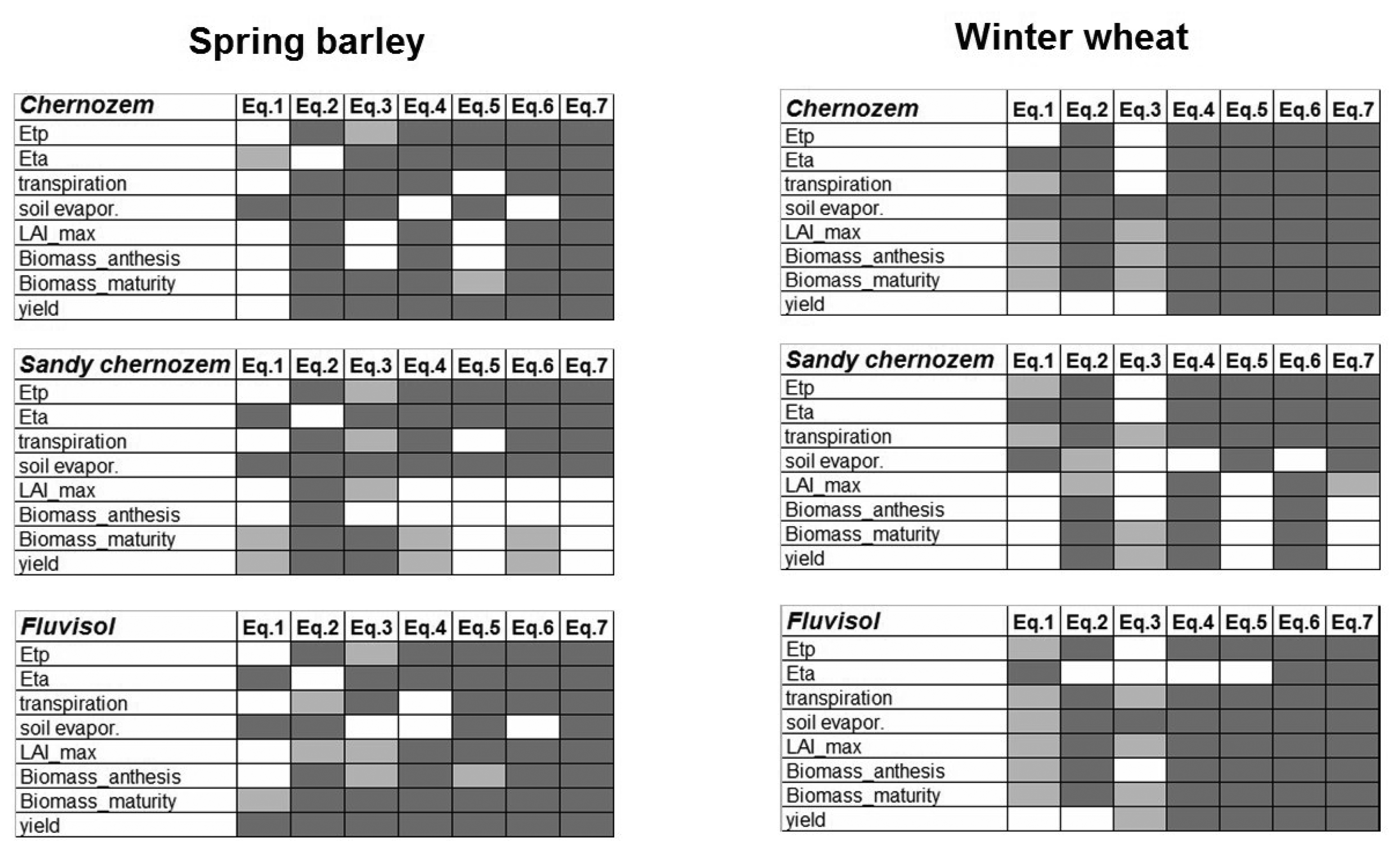
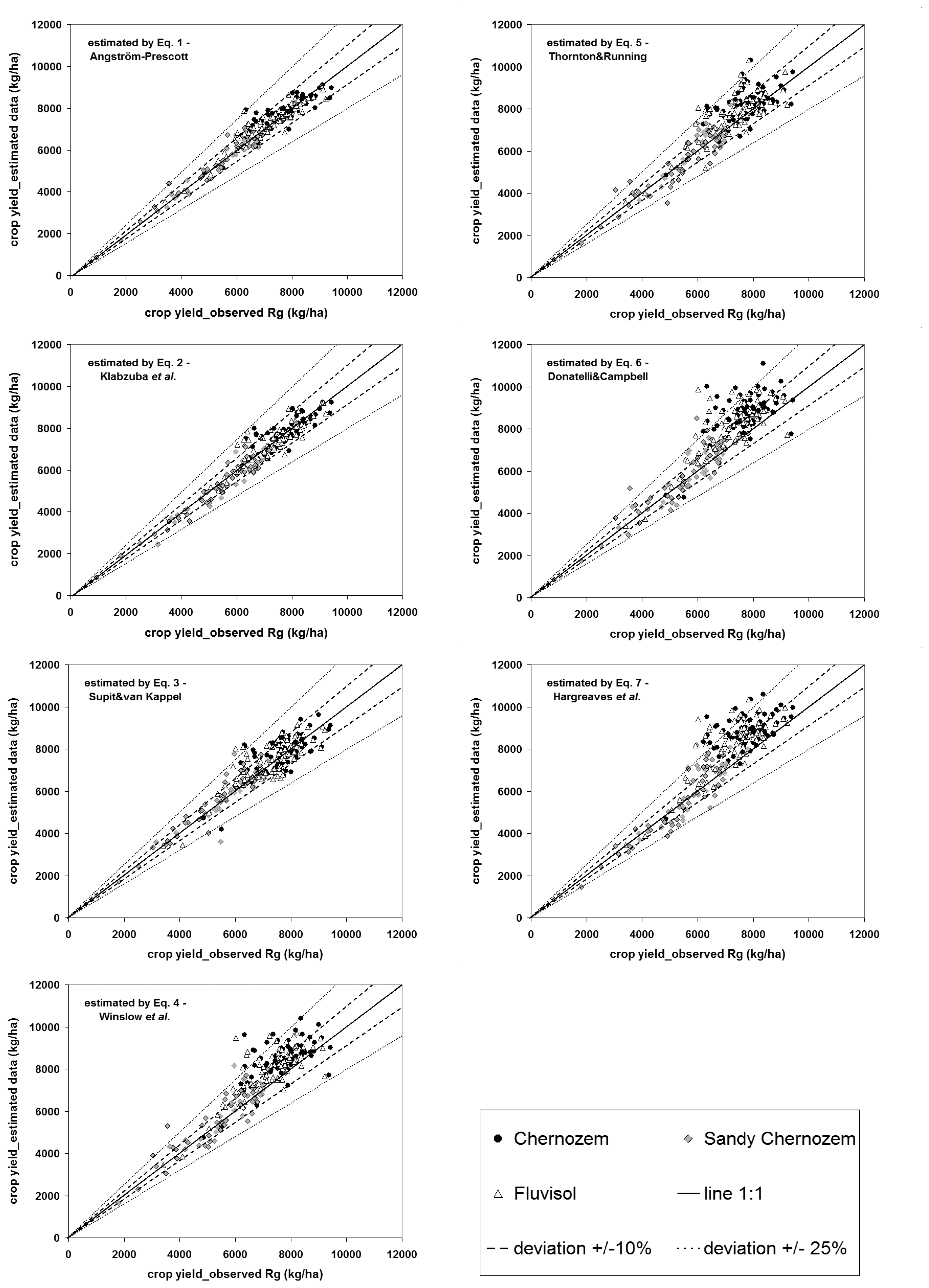
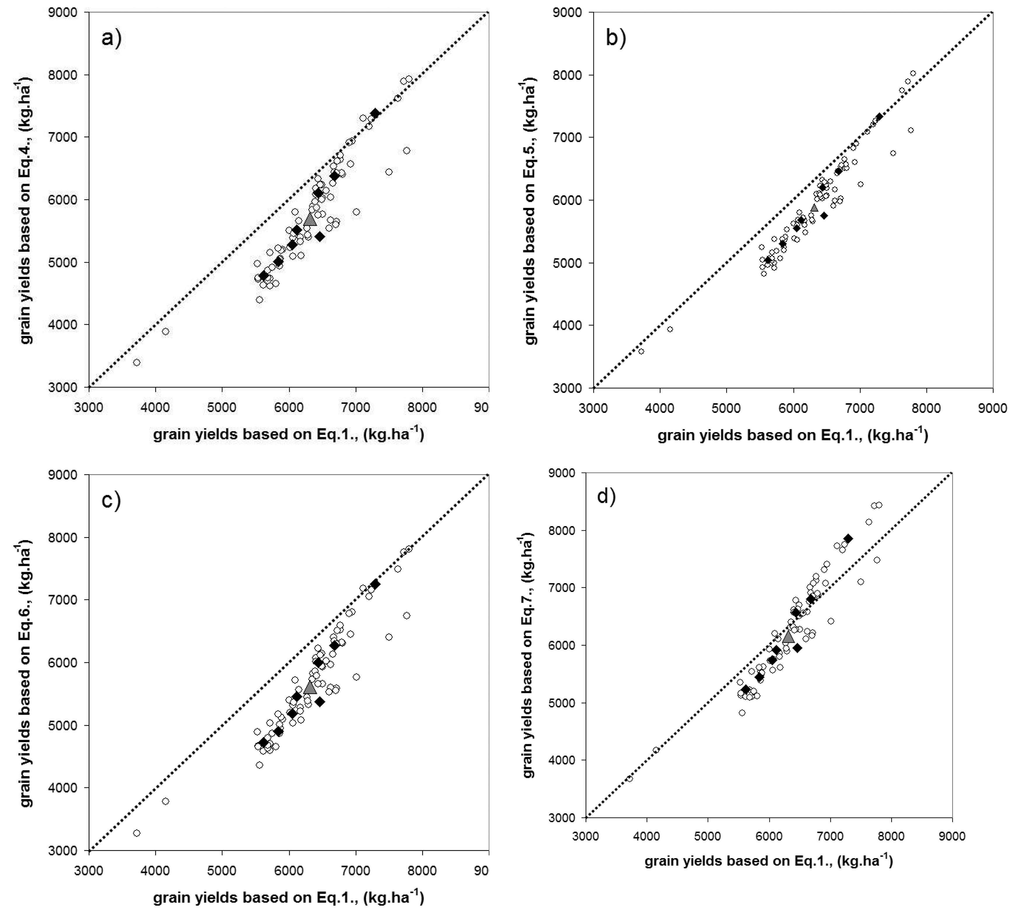
3.1. Site Specific Analysis: Spring Barley

As can be seen in Table 1 and Figure 2, Eqs. (1) and (2) provide estimates of R_G with relatively low bias especially compared with methods based on the diurnal temperature range. At the same time we found that the results varied greatly with the soil type and that the majority of the tested R_G methods produced statistically significant differences compared with the control runs. As expected, Eq. (1) performed best of all methods and the crop model outputs in most cases did not significantly differ from the simulations based on the observed R_G. We found that the differences in crop model outputs caused by the R_G were more pronounced in fluvisol and especially in chernozem (i.e. the prime agricultural soil type). The low sensitivity of sandy chernozem can be explained by the much higher crop water stress on this particular soil that was noted during most of the 97 simulated seasons. As soon as water stress becomes the dominant limiting factor, it suppresses growth processes and decreases the overall effect of differences in R_G values. It is not surprising that the R_G estimation methods based on sunshine duration (i.e. Eq. (1)-(2) showed relatively good agreement when used for the CERES-Barley crop model compared with the observed R_G values (Table 4). However, even with the most reliable R_G estimates i.e. Eqs. (1)- (3) yield deviations in individual seasons were sometimes more than ±25 per cent compared with yield simulated with the observed R_G data. The remaining methods showed a three- to ninefold increase in deviations greater than ±25 per cent (Table 4). The soil component again played an important role as the number of seasons with deviations greater than ±10 per cent was about 40 per cent less in the sandy chernozem than in the chernozem and this was also confirmed by the existence of clear patterns when PI was applied.

Further investigation of those seasons during which the yield deviation was greater than ±10 per cent showed no direct correlation between the R_G estimation error and crop yield. However, a strong correlation does exist (Pearson correlation coefficient r > 0.7) between the deviation of transpiration over the season (compared to the control run with observed R_G) and the accumulated difference between estimated and observed R_G at a given site. The final effect of the deviation in R_G value on the actual transpiration (and consequently on grain yield) was in many cases disproportionate, resulting in amplification/attenuation of the deviation caused by the structure of the model algorithm.

It is obvious that an overestimation of R_G leads to enhanced actual evapotranspiration and more intensive photosynthesis if sufficient water is available, resulting in higher LAI_max, biomass and consequently in higher grain yield. On the other hand, the combination of R_G overestimation and the lack of available water will lead to amplification of the water stress and even greater yield decrease. Interestingly, the highest number of significant yield differences caused by the substitution of R_G data was found at the urban sites, i.e. Ostrava-Poruba and Graz, whereas the rural sites (e.g. Gross-Enzersdorf, Kucha ř ovice or Kocelovice) showed 30 or even 50 per cent less error. Trnka et al. [14] showed that at urban sites the precision of the tested methods is lower than at rural sites. This raises the question of whether the data from urban weather stations are suitable for use in crop modelling because owing to increased air pollution, increased air temperatures, etc., neither measured R_G data nor R_G estimates represent conditions outside an urban environment.

3.2. Site Specific Analysis: Winter Wheat

As with the spring barley experiments, Eqs. (1) and (3) worked quite well whilst those based only on air temperature had a much higher error. The only difference compared with the spring barley study was better overall performance of Eq. (4) compared with Eq. (5). Analyses of the CERES-Wheat model outputs (Fig. 2) show that none of the R_G estimation methods produced results that would completely match those based on observed data. Eq. (1) ranked best followed by Eq. (3). The relative difference between the soil types and particular methods were similar for all three soil profiles. This might be explained by the fact that the effect of water stress did not play such a dominant role as in the case of spring barley. It is not surprising that Eq. (1) and Eq. (3) with the lowest values of MBE showed good agreement compared with the observed R_G values, whilst Eqs. (6)- (7)) produced an overall grain yield overestimation, high random error and low correlation with the values compared with the control crop model runs with observed R_G.

The effects of biases in estimated R_G on the total biomass at anthesis was similar to those noted in with grain yields. The bias in wheat yields increased proportionately to the bias in the R_G estimate and was more than ten times higher with Eq. (7) than with Eq. (1). The statistical tests proved that differences between yields based on observed and estimated R_G data are significant for all methods except Eq. (1), which performed satisfactorily on all soil types. As is apparent from Fig. 3 and also

Table 5. The same as the Table 4 but for the CERES-Wheat model. The results are based on the pooled data from the 8 observational sites with total 77 complete years of weather record and three soil types i.e. 231 simulation runs.

Parameter	Eq. (1)	Eq. (2)	Eq. (3)	Eq. (4)	Eq. (5)	Eq. (6)	Eq. (7)
TRANSPIRATION
a)R2	0.90	0.87	0.69	0.61	0.62	0.58	0.60
b)Sl	1.01	1.03	1.02	1.08	1.07	1.10	1.12
c)MBE	1.4	3.4	2.1	8.3	7.2	10.6	12.9
d)RMSE	4.5	6.1	8.2	12.3	11.7	14.3	15.9
e)RMSER	1.1	3.2	1.7	7.8	6.8	10.2	12.6
LAI_max
a)R2	0.94	0.89	0.82	0.75	0.73	0.74	0.76
b)Sl	1.01	1.06	1.02	1.08	1.10	1.10	1.14
c)MBE	1.3	5.7	2.2	9.2	10.8	11.1	15.1
d)RMSE	5.6	9.7	10.0	14.7	16.7	16.1	19.2
e)RMSER	1.0	6.0	1.7	8.7	10.7	10.7	15.1
BIOMASS_MATURITY
a)R2	0.94	0.92	0.84	0.80	0.81	0.79	0.81
b)Sl	1.01	1.01	1.02	1.07	1.05	1.09	1.11
c)MBE	1.1	1.1	1.9	7.3	5.4	9.2	10.8
d)RMSE	4.2	5.3	7.4	11.2	10.2	12.9	14.9
e)RMSER	0.9	1.2	1.6	7.3	5.5	9.3	11.2
YIELD
a)R2	0.93	0.91	0.83	0.80	0.81	0.78	0.80
b)Sl	1.01	0.99	1.02	1.08	1.04	1.10	1.11
c)MBE	0.8	-0.7	2.0	8.0	4.2	9.9	10.4
d)RMSE	4.7	5.5	7.8	11.8	9.4	13.8	14.5
e) RMSER	0.6	0.7	1.8	8.1	4.2	10.1	11.0
proportion of deviation > ± 10%	5.0	10.3	19.1	32.3	22.7	39.0	41.8
proportion of deviation > ± 25%	0.4	0.0	2.1	5.3	3.9	7.4	9.9

Note:

^a)Values of coefficients of determination of the linear regression line with the best fit.

^b)Values of slope of the regression line forced through the origin.

^c)Relative value of the mean bias error expressed in %.

^d)Relative value of the root mean square error expressed in %.

^e)Random component of RMSE (Component of RMSE that is not correctable by linear transformation) expressed in %.

, even the estimates based on Eq. (1) show possibility of yield deviations in excess of ±25 per cent. At the same time Eqs. (4)- (7) resulted in 23 to 42 per cent of the yields being simulated with an error greater than ±10 per cent. The similar effect was noted in case of total biomass at maturity (Annex 2).

The highest number of significant deviations from the simulation runs using estimated R_G was again found on the most fertile soils i.e. chernozem and fluvisol (Fig. 3). We found a similar relationship between the bias in R_G estimate and its propagation through actual transpiration estimates to grain yields as in the case of spring barley. At the same time it should be mentioned that even very high differences between the observed R_G values and estimated ones from November to February did not significantly affect the performance of the crop model. This is evidently the result of winter wheat dormancy during this period. The bias in R_G values from March to July proved to be decisive in terms of overall bias, whilst inaccuracies in R_G estimates in September and October played a negligible role. As with spring barley, at urban sites winter wheat simulations showed proportionally more yield deviations (over ±10 per cent) compared with rural stations.

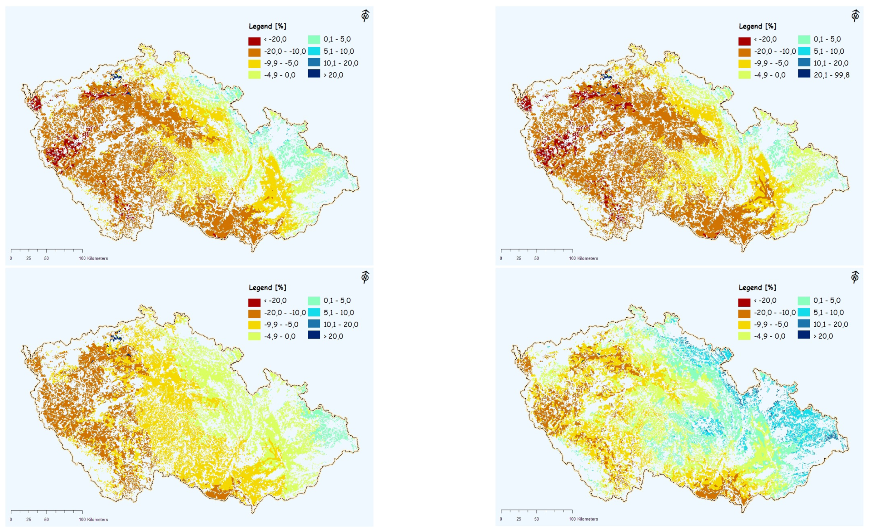
3.3. Spatial Analysis: Winter Wheat

We first compared the mean simulated national winter wheat yield with the long-term statistical data based on the mean national yields during the period 1981-2000 as reported by the Czech Statistical Office (CSO). We found that the mean water-limited yield estimated by WOFOST (as average of all arable soil grids) using Eq. (1) R_G data was 6426 ± 1193 kg/ha. This is about one third higher than the mean national yields reported by the CSO of 4706 ± 373 kg/ha. However, it should be borne in mind that the WOFOST model takes into account only the influence of water stress and does not fully account for the effect of nutrient (especially nitrogen) stress.

In addition WOFOST simulations on the assumption that farmers adhere to good farming practices (i.e. proper crop rotation, soil tillage and plant protection, etc.). In this sense the WOFOST yield prediction could be considered as the maximum attainable yield under given weather and soil conditions assuming optimum fertilisation, plant protection and crop management. These conditions are usually kept in the Official Variety Tests that are regularly performed by the State Institute for Agriculture Supervision and Testing of the Czech Republic. We therefore compared the mean winter wheat yields in the database from all tested winter wheat varieties at 35 sites during period the 1971-2000 (i.e. 12,234 yield records in total) and found that the mean attainable winter wheat yield level in these tests is 6830 ± 1740 kg/ha). As the majority of the experimental stations are located on prime sites within each region, the yields obtained at these sites tend to be skewed to higher values compared with those simulated by WOFOST that take account of arable land in the entire country. The spatial analysis also showed that the WOFOST model in general overestimates the importance of water stress compared with significant environmental stressors (e.g. nitrogen availability, frost damage) and consequently it indicates unrealistically high yields at altitudes above 500 m. At the same time it tends to underestimate yields in the driest parts of the country (i.e. south-east and north-west). As the agricultural areas that are located higher than 500 m above sea level have only marginal importance for overall winter wheat production, we assumed that this tendency could be neglected. Despite all the caveats that are inherent to the WOFOST model (and also in the spatial analysis method) we found surprisingly good agreement between the mean observed yields during the period 1981-2000 and WOFOST estimates at the NUTS4 level, at least in the key cereal growing regions (r = 0.76). However this was true only when the R_G data were obtained via Eq. (1).

A previous comparison of methods based on Eqs. (4)- (7) with the results of Eq. (1) showed highly significant differences in the R_G values. This bias was carried over to estimates of mean yields at the level of individual grids (Fig. 4.) and to the yield estimates aggregated over various categories of NUTS regions (Fig. 5). All four methods led to lower national mean yield than Eq. (1) and the differences were quite high, reaching over 600 kg/ha when Eq. (6) was used. Surprisingly the least reliable method from the preceding site analysis, i.e. Eq. (7), showed the lowest overall bias compared with the reference method in the spatial analysis. As can be seen from Fig. 4, the use of R_G data estimated by Eqs. (4) and (5) resulted in yield biases of more than 20 per cent in many areas. The remaining two methods produced errors of smaller magnitude, but even then the deviations were higher than 10 per cent. The R_G values over the winter wheat growing season estimated by Eqs. (4)-(7) were higher in most locations than estimates based on Eq. (1). As the productivity of most of lowland sites is limited by available water, the higher R_G values consequently lead to higher soil evaporation as well as increased water uptake by the crop and faster depletion of soil water reserves. This resulted in higher water stress and lower crop yields in most seasons. Most of the grids with unsatisfactory results are located in the western part of the country (Fig. 4).

We found that bias of Eq. (4) and (5) R_G estimates compared with the control values (Eq. 1) showed a significant correlation with the altitude and longitude of the station (Fig 4a-4b). At the same time the analysis of the residuals using PI revealed the existence of distinct regional clusters with similar magnitudes of error. This led us to the conclusion that the unsatisfactory performance of Eq. (4) and Eq. (5) could be attributed to i) the insufficient accommodation of the altitude influence on the relationship between daily diurnal temperature range, precipitation and daily sum of global radiation; ii) the changing character of the overall climate in longitudinal direction; and iii) regional specific climatic conditions. Whereas the first factor can be eliminated by recalibration of the methods, the remaining two seem to be intrinsic to the methods themselves. Both Eqs. (4) and (5) rightly consider occurrence of precipitation as a measure of the cloudiness, and R_G on rainy days is proportionately lower. Consequently these methods will perform less well at sites with a high number of cloudy or foggy days without precipitation. Such days are in fact more common in the western part of the country, where the maritime climate has a stronger influence of in combination with the rain shadow of the Ore mountains [76]. This means that despite higher overall cloudiness, the total amount of precipitation is smaller than in the corresponding areas in the eastern part of the country.

Added to this is the much lower number of clear days and the above average occurrence of foggy days in the valleys of western and southern Bohemia [76]. In some areas these climate-related factors are combined with anthropogenic pollution of the atmosphere by solid particles and aerosols, which further decreases the incoming R_G and can potentially influence agriculture productivity [77].

When data based on Eqs. (4)- (5) were then used as inputs for the WOFOST model, it led to much greater water requirements than in reality. This was particularly pronounced in areas with below average precipitation. The error was multiplied further on shallow or sandy soils (which are more common in the south-western part), leading to complete crop failure in some seasons. The unsatisfactory results of the spatial analysis based on Eq. (6) R_G data could be explain by the high variability in the method performance at the individual sites. Whilst at some sites the R_G values were significantly underestimated compared with Eq. (1), the opposite behaviour was noticed at other sites regardless of the station altitude and geographical location. The behaviour could be explained by the method used for parameterisation of Eq. (6), which had been extensively tested under conditions in northern Italy but not those prevalent in Central Europe. The surprisingly good results achieved with Eq. (7) might be attributed to the fact that it did not show any trend in the biases of R_G estimates and the mean error was smaller than in case of Eq (6) as the parameterisation was based on a pan-European study [10]. However even the estimates based on Eq (7) systematically underestimated the R_G values by more than 18 per cent at some sites whilst at other locations they were overestimated by 7 per cent with errors in winter wheat yields in a similar range (Fig 4d). Large differences between production levels among the five tested equations can be overviewed at Fig. 5, which shows that bias introduced to the WOFOST simulation might be indeed quite high and is not diminished by further aggregation of the model outputs to the NUTS 4, NUTS2 or even NUTS 0 level.

4. Discussion

Although the propagation of the error in R_G estimates (e.g. calculation of evapotranspiration or crop yields in crop models) has already been analysed in previous works [24, 36, 38, 78-81]. Research carried out by Llasat and Snyder [80] or Xie et al. [81] concluded that the effect of error in the R_G daily estimate caused relatively small changes to the final model output, which was either potential evaporation or county crop yield. They reported that the R_G overestimation by 4 per cent caused an error in the potential evapotranspiration of between 1.6 and 3.6 per cent depending on the time of the year [80]. Lindsey and Farnsworth [79] found that the use of cloud cover as an R_G predictor usually led to an underestimation of the potential evaporation from a water surface by 14 per cent on average. In some cases these authors reported an error as large as 39 per cent, which is a significantly worse performance than any of the seven methods tested in our study.

The effect of the systematic error in the R_G estimates on the simulated spring wheat yield was examined by Nonhebel [16], who had found that the overestimation of the R_G values by 10 per cent led to a 5 per cent increase in the potential yield, while the underestimation by the same percentage would simulate yield to be 9 per cent lower. In the case of water-limited yields Nonhebel [16] reported an inverse relationship between R_G and spring wheat grain yield. Brown and Rosenberg [39] reported that dry land wheat yields predicted by the EPIC model in the MINK region increased by 5 per cent with increasing R_G values (+15 per cent) and vice versa. It should be noted that the magnitude of the change in the simulated wheat yield was approximately one third of the imposed R_G deviation. The same results were reported for the seasonal actual evapotranspiration. All these studies considered the uniform systematic error in input R_G data throughout all growing seasons. In reality, the R_G estimation error varies greatly during individual months (and even days) of the growing season [14] making it much harder to estimate the final impact solely on the basis of the MBE or RMSE values of the R_G estimate. Our findings have major implications for site model calibration when estimates other than measured values or sunshine duration based R_G estimates are used. It is clear that the high probability of model bias larger than 10 per cent caused by imprecise R_G estimates in combination with the random component of the bias might lead to misleading parameterisation of the model. The input parameters might be optimised for unrealistic yield levels, thus compromising further model use. It is also questionable whether crop model that have been calibrated with the use of measured R_G data (or estimates based on Eq. (1)) can be used without further calibration when R_G is estimated by other methods (e.g. Eqs. (4)- (7)).

This conclusion is valid at least in the Central European conditions as other authors considered uncertainties in R_G values being insignificant e.g. [34]. However, this particular study was done in the subtropical and tropical climate of India. On the other hand, results of ALMANAC, i.e. another crop growth model [82], showed significant variability in rain‐fed maize yields in eight Texas counties (−12 per cent to +17 per cent) when the R_G value was decreased by 11 per cent during the growing season. When the R_G value was increased by 10 per cent the yields varied from between −8 and +3 per cent of the original values [81], even though the observed R_G values were modified by a constant multiplier and thus missing the random component of the bias. De Jong and Stewart [36] used estimated R_G values based on the diurnal temperature range and daily total precipitation (with the relative RMSE during the growing season of between 10.7 and 14.3 per cent) in the WOFOST crop model [58]. The difference in the wheat yield obtained with observed and estimated R_G expressed in terms of RMSE was on average 344 to 643 kg.ha^-1, depending on the location. However, it should be noted that the authors of the Canadian study considered the “potential yield” (no effect of water and nutrient stress was considered). The study reported that more than 88 per cent of potential yields were simulated with deviation smaller than ±15 per cent compared with runs with observed R_G data, which broadly corresponds with results of our study (considering results of Eqs. (4) and (5).

Pohlert [38] showed that the use of the Ångström-Prescott formula (Eq. 1) in WOFOST models produces very similar results compared with the observed R_G in a Mediterranean environment. He also proved that the performance of empirical radiation models is highly dependent on the locality and the production level of the model. Another study by Rivington [18] performed in southern England concluded that the crop model (CropSyst) performed well when the R_G estimates were based on the sunshine duration hours or on data from the similar proxy meteorological station. Eq. (6) ranked as the last option, but each of the tested methods showed a significant annual yield deviation of a magnitude comparable to the present study. It highlights the necessity for careful interpretation of any crop model output based on estimated climatic data. Based on the presented facts it might concluded that if sunshine duration hours are used as a predictor of R_G values, the overall results (based on a large number of simulations at different sites) will be minor. However, if the crop model is used for site‐specific yield forecasting, the even application of this best available method might yield deviations in excess of ±25 per cent in some cases.

The uncertainty in the seasonal simulation results increases with R_G estimation methods based on other weather variables. These findings partly support the initial hypothesis of the study that the inaccuracies in the R_G input data might be attenuated in some seasons but multiplied in others owing to the non-linear character of crop model relationships. Witt et al. [42] reported that the effect of uncertainty in R_G data might be partly mitigated by aggregation of the results over the whole territory (e.g. Germany or France). However, this effect played only marginal role in our study (Fig. 5), mainly because of the different method of obtaining regional crop yields. Whereas our study relied solely on the WOFOST model, Witt et al. [42] used Crop Growth Monitoring Systems, where WOFOST outputs are coupled with the results of national statistics, which according to our opinion significantly reduces the magnitude of an error introduced by uncertainties in the crop model inputs.

It seems obvious that the possibility of significant seasonal variation in the yields based on the estimated R_G compared with control runs does not apply only to CERES or WOFOST crop models or process-oriented models in general. In our view statistical or parsimonious models [8, 9, 68] that use the R_G as independent variable might also be affected by the inaccuracies of the R_G estimate, and additional analysis of the error propagation should be carried out. Another field where the present results should be taken into account is in climate change impact studies that are largely based on the crop models. For example for 2050 most of the climate change scenarios predict seasonal R_G changes in Central Europe ranging from −5 to +7 per cent [83]. Such estimates are additionally loaded with quite a high degree of uncertainty given the relatively poor performance of the GCMs in the evaluation process. As has shown, errors of this magnitude could in some cases alter the overall results of such studies. In our view there is therefore a great need for further research aimed at the development of more precise and widely applicable method(s) for spatially estimates of daily R_G based more on the underlying physical principles and using routinely available data.

One of the possibilities might be to include multiple values of commonly measured weather variables (e.g. temperature and water vapour pressure) per each day in combination with daily precipitation total or cloud cover values, improvements to remote sensing methods and above all an increase the density of the R_G monitoring sites. At the same time more reliable estimates of R_G changes under expected climatic conditions should be developed to increase the accuracy of subsequent studies. In the meantime, detailed sensitivity analyses that would test model behaviour over the range of R_G data uncertainty are strongly recommended in studies based on crop models.

5. Conclusions

The results of previous studies suggest that estimated R_G values are loaded with error, which might compromise the precision of the subsequent crop model applications both on the site and at the regional level. Therefore a detailed site analysis of the error propagation was made first using two crop models, namely CERES-Barley and CERES-Wheat. We found that even the method yielding the lowest bias in R_G estimates (Ångström-Prescott (Eq. 1)) influences a number of key crop model outputs. The precision of the yield estimates and other crop model outputs is lower but still acceptable when estimates based on the diurnal temperature range and cloud cover (Supit and van Kappel, (Eq. 2)) are used. Methods based on the diurnal temperature range and total precipitation yielded better model estimates than those based on temperature extremes, but there was a systematic bias in the spring barley and winter wheat yields and the considerable increase in seasons with yield departure of more than ±25 per cent. The use of methods based solely on the diurnal temperature range for the purposes of seasonal yield forecasting or climate change impact assessment is questionable, as there is a very high probability of significant yield departure (and of systematic error). The most productive soils (e.g. chernozem) seem to be the most prone to amplification of systematic and random errors in the R_G data, which has serious implications both for yield monitoring and determining region production potential.

The spatial assessment of the R_G data uncertainty propagation over the winter wheat yields also revealed significant differences within the study area. We found that R_G estimates based on diurnal temperature range or its combination with daily total precipitation (Eqs. (4)- (7)) would in some regions produce up to 30 per cent bias in the mean winter wheat grain yields compared with the simulations done with R_G values estimated by Eq. (1). Contrary to the results at individual sites, Eqs. (4) and (5) showed significantly poorer performance compared with Eq. (7). This was caused by the marked increase in the R_G estimate bias with altitude and longitude of the location because of subtle changes in the overall climatology. We also concluded that calibration of the model with data other than those based on the observed values or hours of sunshine might lead to an inappropriate model setting. At the same time use of the model with R_G estimated by various methods might cause significant misinterpretation of the model results, as the effect of the uncertainty in the R_G values cannot be easily estimated. These findings in our view should act as an incentive to further research aimed at the development of more precise and widely applicable methods of estimating daily R_G based more on the underlying physical principles. One of the possibilities might be the utilisation of more measurements per day of commonly collected weather variables (e.g. temperature and water vapour pressure) in combination with daily precipitation total or term cloud cover values.

It should be stressed that the application of input data intensive methods is no longer limited by the power of available computers and even large databases can be handled easily on commonly available equipment. The second option lies in making empirical coefficient values required by most of the tested R_G methods accessible in higher resolution than at present. Studies that followed the example of [10] should therefore be undertaken on both a European and a global scale. This would permit users to select themselves of the most suitable methods for a particular set of conditions without the need for calibration, thus ensuring reasonable precision. An overall decrease in the existing uncertainties in the R_G estimates would result in an increase in the reliability of subsequent applications that use the R_G as input variable. Finally, as precise and reliable sensors for direct measurement of R_G are becoming more readily available, the density of the radiation measurement sites should be increased, especially in regions with high spatial R_G heterogeneity.

References and Notes

1. Wit de, C.T.; Penning de Vries, F.W.T. Predictive models in agricultural production. Phil. Trans. R. Soc. London B 2005, 310, 309–315. [Google Scholar]
2. Aggarwal, P.K. Application of systems simulation for understanding and increasing yield potential of wheat and rice. Ph.D. Thesis, Wageningen Agriculture University, 2000; p. 176. [Google Scholar]
3. Diepen van, C.A. An Agrometeorological model to monitor the crop state on a regional scale in the European Community: Concept implementation and first operational outputs. Proceedings of the Conference on Application of Remote Sensing to Agricultural Statistics, Belgirate, Italy; 1992; pp. 269–277. [Google Scholar]
4. Perdigão, V.; Suppit, I. (Eds.) An Early Crop Yield Estimation Method for Finnish Conditions: The crop growth monitoring system of the Joint Research Centre with and without Remotely Sensed and other Additional Input data; EUR-18975 EN 1999; p. 144.
5. Wolf, J.; Evans, L.G.; Semenov, M.A.; Eckersten, H.; Iglesias, A. Comparison of wheat simulation models under climate change I Model calibration and sensitivity analyses. Climate Research 1996, 7, 253–270. [Google Scholar]
6. Alexandrov, A.; Hoogenboom, G. The impact of climate variability and change on crop yield in Bulgaria. Agric. For. Meteorol 2000, 104, 315–327. [Google Scholar]
7. Izaurralde, R.C.; Rosenberg, N.J.; Brown, R.A.; Thomson, A.M. Integrated assessment of Hadley Center (HadCM2) climate change impacts on agricultural productivity and irrigation water supply in the conterminous United States Part II Regional agricultural production in 2030 and 2095. Agric. For. Meteorol 2003, 117, 97–122. [Google Scholar]
8. Landau, S.; Mitchell, R.A.C.; Barnett, V.; Colls, J.J.; Payne, C.J. A parsimonious multiple-regression model of wheat yield response to environment. Agric. For. Meteorol 2000, 101, 151–166. [Google Scholar]
9. Han, D.; O'Kiely, P.; Sun, D.W. Application of Water-stress Models to estimate the Herbage Dry Matter Yield of Permanent Grassland Pasture Sward Regrowth. Biosystem Engineering 2003, 84, 101–111. [Google Scholar]
10. Supit, I.; van Kappel, R.R. A simple method to estimate global radiation. Solar Energy 1998, 63, 147–160. [Google Scholar]
11. Liu, D.L.; Scott, B.J. Estimation of solar radiation in Australia from rainfall and temperature observations. Agric. For. Meteorol 2001, 106, 41–59. [Google Scholar]
12. Rivington, M.; Bellocchi, G.; Matthews, K.B.; Buchan, K. Evaluation of three model estimations of solar radiation at 24 UK stations. Agric. For. Meteorol 2005, 132, 228–243. [Google Scholar]
13. Oesterle, H. Reconstruction of Daily Global Radiation for Past Years for use in Agricultural Models. Phys. Chem. Earth. 2001, 26, 253–256. [Google Scholar]
14. Trnka, M.; Žalud, Z.; Eitzinger, J.; Dubrovský, M. Quantification of uncertainties introduced by selected methods for daily global solar radiation estimation. Agric. For. Meteorol 2005, 131, 54–76. [Google Scholar]
15. Thornton, P.E.; Running, S.W.; White, M.A. Generating surfaces of daily meteorological variables over large regions of complex terrain. Journal Hydrol. 1997, 190, 214–251. [Google Scholar]
16. Nonhebel, S. The importance of weather data in crop growth simulation models and assessment of climate change effects. Ph.D. Thesis, Agriculture University, Wageningen, 1993; p. 144. [Google Scholar]
17. Hunt, L.A.; Kuchar, L.; Swanton, C.J. Estimation of solar radiation for use in crop modeling. Agric. For. Meteorol 1998, 91, 293–300. [Google Scholar]
18. Rivington, M.; Matthews, K.B.; Buchan, K. A comparison of methods for providing solar radiation data to crop models and decision support systems. In Integrated Assessment and Decision Support, Proceedings of the 1st biennial meeting of the International Environmental Modeling and Software Society, Lugano, Switzerland, Jun 24-27, 2002; Rizzoli, A.E., Jakeman, A.J., Eds.; iEMSs: Manno, Switzerland, 2002; 3, pp. 193–198. [Google Scholar]
19. Marion, W.; George, R. Calculation of Solar Radiation Using a Methodology with Worldwide Potential. Solar Energy 2001, 71, 275–283. [Google Scholar]
20. Wyser, K.O.; Hirok, W.; Gautier, C.; Jones, C. Remote sensing of surface solar irradiance with correction for 3-D cloud effect. Remote Sensing of Environment 2002, 80, 272–284. [Google Scholar]
21. Richardson, C.W. Stochastic simulation of daily precipitation temperature and solar radiation. Water Resources Res. 1981, 17, 182–190. [Google Scholar]
22. Dubrovský, M. Creating daily weather series with use of the weather generator. Environmetrics 1997, 8, 409–424. [Google Scholar]
23. Hansen, J.W. Stochastic daily solar irradiance for biological modeling applications. Agric. For. Meteorol 1999, 94, 53–63. [Google Scholar]
24. Soltani, A.; Meinke, H.; de Voil, P. Assesing linear interpolation to generate daily radiation and temperature data for use in crop simulations. Europ. J. Agron. 2004, 21, 133–148. [Google Scholar]
25. Safi, S.; Zeroual, A.; Hassani, M. Prediction of global daily solar radiation using higher order statistics. Renewable Energy 2002, 27, 647–66. [Google Scholar]
26. Elizondo, D.; Hoogenboom, G.; McClendon, R.W. Development of a Neural Network Model to Predict Daily Solar Radiation. Agric. For. Meteorol 1994, 71, 115–132. [Google Scholar]
27. Reddy, K.S.; Ranjan, M. Solar resource estimation using artificial neural networks and comparison with other correlation models. Energy Conversion and Management 2003, 44, 2519–2530. [Google Scholar]
28. Ångström, A. Solar and terrestrial radiation. QJR Meteorol. Soc. 1924, 50, 121–125. [Google Scholar]
29. Klabzuba, J.; Bureš, R.; Ko žnarová, V. Model výpo Čtu denních sum globálního zá ření pro pou žití v r ůstových modelech. Proceedings of the “Bioklimatologické pracovné dni 1999 Zvolen” 1999, 121–122. [Google Scholar]
30. Winslow, J.C.; Hunt, E.R.; Piper, S.C. A globally applicable model of daily solar irradiance estimated from air temperature and precipitation data. Ecol. Modeling 2001, 143, 227–243. [Google Scholar]
31. Brisson, N.; Gary, C.; Justes, E.; Roche, R.; Mary, B.; Ripoche, D.; Zimmer, D.; Sierra, J.; Bertuzzi, P.; Burger, P. An overview of the crop model STICS. European Journal of Agronomy 2003, 18, 309–332. [Google Scholar]
32. Van Dam, J.C.; Huygen, J.; Wesseling, J.G.; Feddes, R.A.; Kabat, P.; van Walsum, P.E.V.; Groenendijk, P.; van Diepen, C.A. Theory of SWAP version 20; Report #71; Department of Water Resources Wageningen Agricultural University, 1997; p. 167. [Google Scholar]
33. Donatelli, M.; Bellochi, G.; Fontana, F. RadEst300: software to estimate daily radiation data from commonly available meteorological variables. European Journal of Agronomy 2003, 18, 363–367. [Google Scholar]
34. Aggarwal, P.K. Uncertainties in crop soil and weather inputs used in growth models implications for simulated outputs and their applications. Agricultural Systems 1995, 48, 361–384. [Google Scholar]
35. Metselaar, K. Auditing predictive models: a case study in crop growth. Ph.D. Thesis, University of Wageningen, 1999; p. 265. [Google Scholar]
36. De Jong, R.; Stewart, D.W. Estimating global solar radiation from common meteorological observations in western. Canada Can. J. Plant. Sci. 1993, 73, 509–518. [Google Scholar]
37. Iziomon, M.G.; Mayer, H. Performance of solar radiation model4s-a case study. Agric. For. Meteorol 2001, 110, 1–11. [Google Scholar]
38. Pohlert, T. Use of empirical global radiation models for maize growth simulations. Agric. For. Meteorol 2004, 126, 47–58. [Google Scholar]
39. Brown, A.R.; Rosenberg, N.J. Sensitivity of crop yield and water use to change in a range of climatic factors and CO2 concentrations: a simulation study applying EPIC to the central USA. Agric. For. Meteorol 1997, 83, 171–203. [Google Scholar]
40. Supit, I.; van der Goot, E. National wheat yield prediction of France as affected by the prediction level. Ecological Modeling 1999, 116, 203–223. [Google Scholar]
41. Saariko, R.A. Applying a site based crop model to estimate regional yields under current and changed climate. Ecological Modeling 2000, 131, 191–206. [Google Scholar]
42. Wit de, A.J.W.; Boogard, H.L.; van Diepen, C.A. Spatial resolution of precipitation and radiation: The effect on regional crop yield forecasts. Agric. For. Meteorol 2005, 135, 156–168. [Google Scholar]
43. Audsley, E.; Pearn, K.R.; Simota, C.; Cojocaru, G.; Koutsidou, E.; Rounsevell, M.D.A.; Trnka, M.; Alexandrov, V. What can scenario modeling tell us about future European scale land use and what not? Environmental Science and Policy 2006, 9, 148–162. [Google Scholar]
44. Dobesch, H.; Mohnl, H. Comparison of Time Series of Sunshine Duration Measured by the Campbell-Stokes Recorder and the Haenni Solar System. In Instruments and Observing Methods Report No 49 WMO/TD-No 462 WMO, Technical Conference on Instruments and Methods of Observation (TECO 92); Wien, Austria, 1992; pp. 260–265. [Google Scholar]
45. Schöner, W.; Mohnl, H. Homogeneity of Austrian Sunshine Duration Data Sets. 2nd International Conference on Experiences with Automatic Weather Stations (ICEAWS 1999 27 to 29 September 1999 Vienna) Österreichische Beiträge zu Meteorologie und Geophysik Heft Nr 20/PublNr 387 (CD-ROM), Vienna Austria; 1999; p. 5. [Google Scholar]
46. Stanhill, G.; Cohen, S. Global dimming: a review of the evidence for a widespread and significant reduction in global radiation with discussion of its probable causes and possible agricultural consequences. Agric. For. Meteorol 2001, 107, 255–278. [Google Scholar]
47. Allen, R.G.; Pereira, L.S.; Raes, D.; Smith, M. In Crop evapotranspiration: Guidelines for computing crop requirements; Irrigation and Drainage. Paper No. 56; FAO: Rome, Italy, 1998; p. 300. [Google Scholar]
48. Prescott, J.A. Evaporation from a water surface in relation to solar radiation. Trans. R. Soc. South Australia 1940, 64, 114–118. [Google Scholar]
49. Wörner, H. Zur Frage der Automatisierbarkeit der Bewölkungsangaben durch Verwendung von Strahlungsgröβen. Abh. Met. Dienst DDR 1967, 11, 82. [Google Scholar]
50. Hargreaves, G.L.; Hargreaves, G.H.; Riley, P. Irrigation water requirement for the Senegal River Basin. Journal of Irrigation and Drainage Engineering ASCE 1985, 111, 265–275. [Google Scholar]
51. Thorton, P.E.; Running, S.W. An improved algorithm for estimating incident daily solar radiation from measurements of temperature humidity and precipitation. Agric. For. Meteorol 1999, 93, 211–228. [Google Scholar]
52. Bristow, K.; Campbell, G.S. On the relationship between incoming solar radiation and daily maximum and minimum temperature. Agric. For. Meteorol 1984, 52, 275–286. [Google Scholar]
53. Donatelli, M.; Marletto, V. Estimating surface solar radiation by means of air temperature. In Proceedings of the 3rd Congress of the European Society for Agronomy; Padova, Italy, 1994; pp. 352–353. [Google Scholar]
54. Donatelli, M.; Campbell, G.S. A simple method to estimate global radiation. Proceedings of the 5th ESA conference, Nitra, Slovak Republic; 1998; pp. 133–134. [Google Scholar]
55. Choisnel, E.; de Villele, O.; Lacroze, F. Une aproche uniformisée du calcul de l¨évaporation potentielle por lénsemble de pays de la communauté européene; Publication EUR 14223 FR of the Office for Official Publications of the EU: Luxemburg, 1992. [Google Scholar]
56. Otter-Nacke, S.; Ritchie, J.T.; Godwin, D.C.; Singh, U. A user's guide to CERES Barley - V210 International Fertilizer Development Center Simulation manual IFDC-SM-3. 1991, 87. [Google Scholar]
57. Godwin, D.C.; Ritchie, J.T.; Singh, U.; Hunt, L. A User's Guide to CERES Wheat-V210; International Fertilizer Development Center Muscle Shoals AL USA, 1989; p. 86. [Google Scholar]
58. Diepen van, C.A.; Wolf, J.; Keulen, H. WOFOST: a simulation model of crop production. Soil Use and Management 1989, 5, 16–24. [Google Scholar]
59. Supit, I.; Hooijer, A.A.; van Diepen, C.A. System description of the WOFOST 60 crop simulation model implemented in CGMS. Volume 1 Theory and Algorithms; Joint Research Centre Commission of the European Communities EUR 15956 EN: Luxembourg, 1994; p. 146. [Google Scholar]
60. Boogaard, H.L.; Eerens, H.; Supit, I.; Van Diepen, C.A.; Piccard, I.; Kempeneers, P. Description of the MARS crop yield forecasting system (MCYFS); METAMP report Alterra Wageningen, the Netherlands & VITO Mol, Belgium & Supit Consultancy Houten: The Netherlands, 2002. [Google Scholar]
61. Wolf, J.; van Diepen, C.A. Effects of climate change on grain maize yield potential in the European Community. Climatic Change 1995, 29, 299–331. [Google Scholar]
62. Dubrovský, M.; Trnka, M.; Žalud, Z.; Semerádová, D. Estimating the Crop Yield Potential of the Czech Republic in Present and Changed Climates. Proceedings of the 5th European Conference on Applied Climatology, Nice, France, Sept 27-30, 2004; p. 315.
63. Ritchie, J.T.; Singh, U.; Godwin, D.C.; Bowen, W.T. Cereal growth development and yield. In Understanding Options for Agricultural Production; Tsuji, G.Y., Hoogenboom, G., Thorton, P.K., Eds.; Kluwer Academic Publishers: Dodrecht, The Netherlands, 1998; p. 325. [Google Scholar]
64. Jones, C.A.; Kiniry, N. CERES-Maize A Simulation Model of Maize Growth and Development. Texas A&M; University Press: College Station, TX, 1986; p. 194. [Google Scholar]
65. Tsuji, G.Y.; Hoogenboom, G.; Thornton, P.K. Understanding Options for Agricultural Production; Kluwer Academic Publishers: Dodrecht, The Netherlands, 1998; p. 325. [Google Scholar]
66. Jones, J.W.; Hoogenboom, G.; Porter, C.H.; Boote, K.J.; Batchelor, W.D.; Hunt, L.A.; Wilkens, P.W.; Singh, U.; Gijsman, A.J.; Ritchie, J.T. The DSSAT cropping system model. European Journal of Agronomy 2003, 18, 235–265. [Google Scholar]
67. Eitzinger, J.; Trnka, M.; Hösch, J.; Žalud, Z.; Dubrovský, M. Comparison of CERES WOFOST and SWAP models in simulating soil water content during growing season under different soil conditions. Ecological Modeling Volume 2004, 171, 223–246. [Google Scholar]
68. Trnka, M.; Eitzinger, J.; Gruszczynksi, G.; Burchgraber, K.; Resch, R.; Schaumberger, A. A simple statistical model for predicting herbage production from permanent grassland. Grass and Forage Sciences 2006, 61, 253–271. [Google Scholar]
69. Trnka, M.; Dubrovský, M.; Semerádová, D.; Žalud, Z. Projections of uncertainties in climate change scenarios into expected winter wheat yields. Theoretical and Applied Climatology 2004, 77, 229–249. [Google Scholar]
70. Tomášek, M. In P ůdy České republiky; Český geologický ústav. Prague, 2000; p. 67. [Google Scholar]
71. Dubrovský, M.; Žalud, Z.; Trnka, M.; Haberle, J.; Pešice, P. PERUN: the system for seasonal crop yield forecasting based on the crop model and weather generator. Proceedings of XXVII General Assembly of EGS, Nice, France, Apr 21-26 2002.
72. Davies, J.A.; McKay, D.C. Evaluation of selected models for estimating solar radiation on horizontal surfaces. Solar Energy 1989, 43, 153–168. [Google Scholar]
73. Hansen, J.W.; Jones, J.W. Scaling-up crop models for climate variability applications. Agriculture Systems 2000, 65, 43–72. [Google Scholar]
74. Donatelli, M.; Acutis, M.; Bellochi, G.; Fila, G. New Indices to Quantify Patterns of Residuals Produced by Model Estimates. Agronomy Journal 2004, 96, 631–645. [Google Scholar]
75. Fila, G.; Bellocchi, G.; Acutis, M.; Donatelli, M. IRENE: a software to evaluate model performance. Eur. J. Agron. 2003, 18, 369–372. [Google Scholar]
76. Tolasz, R.; Míková, T.; Valeriánová, A. (Eds.) Climatic Atlas of Czechia; Czech Hydrometeorological Institute and Palacky University Olomouc: Prague, Czech Republic, 2007; p. 256.
77. Greenwald, R.; Bergin, M.H.; Xu, J.; Cohan, D.; Hoogenboom, G.; Chameides, W.L. The influence of aerosols on crop production: A study using the CERES crop model. Agriculture Systems 2006, 89, 390–413. [Google Scholar]
78. Meyer, S.J.; Hubbard, K.G.; Wilhite, D.A. Estimating potential evapotranspiration: The effect of random and systematic errors. Agric. For. Meteorol 1989, 46, 285–296. [Google Scholar]
79. Lindsey, S.D.; Farnsworth, R.K. Sources of solar radiation estimates and their effect on daily potential evaporation for use in streamflow modeling. Journal of Hydrology 1997, 201, 348–366. [Google Scholar]
80. Llasat, M.C.; Snyder, R.L. Data error effect on net radiation and evapotranspiration estimation. Agric. For. Meteorol 1998, 91, 209–221. [Google Scholar]
81. Xie, Y.; Kiniry, J.R.; Williams, J.R. The ALMANAC model's sensitivity to input variables. Agricultural Systems 2003, 78, 1–16. [Google Scholar]
82. Kiniry, J.R.; Williams, J.R.; Gassman, P.W.; Debaeke, P. A general process-oriented model for two competing plant species. Trans ASAE 1992, 35, 801–810. [Google Scholar]
83. Dubrovský, M.; Nemešová, I.; Kalvová, J. Uncertainties in Climate Change Scenarios for the Czech Republic. Climate Research 2005, 29, 139–156. [Google Scholar]
Figure 1. Map of the study area with the location of the solar radiation observatories (marked as stars) used as the source of the meteorological data in the site specific simulations. Points within the Czech Republic indicate stations where observed weather data were available for spatial analysis, thin gray lines within the Czech Republic delimit borders of individual NUTS4 regions and the black lines represent NUTS 2 regions both in the Czech Republic and in Austria. The shaded area represents the areas above 750 and 1500 m above the sea level.
Sensors 07 02330f1
Figure 2. Visualization of the statistical significant differences between the crop model runs (CERES-Barley & CERES-Wheat), using the observed RG data (control) and the daily RG estimates based on Eqs. (1)-(7). The white color represents those runs where no statistically significant difference was found; gray color stands for the statistically significant difference at the 5 % level of significance whilst the black color represents the significant difference at 1 % level. The differences were tested by paired t-test, if the distribution was found to be normal (assessed by one sample Kolmogorov-Smirnov test at Lilliefors 5 % significance level) and for non-normally distributed samples by Wilcoxon Signed Rank Test.
Sensors 07 02330f2
Figure 3. Scatter plot charts representing winter wheat yields (CERES-Wheat) during individual seasons simulated using observed RG and those estimates by Eqs. (1)-(7). The results of simulations at three soil types are presented at each chart.
Sensors 07 02330f3
Figure 4. Relative deviations of the winter wheat mean yields (1961-2000) in 1×1 km grids simulated by WOFOST crop model. The mean relative deviation was calculated as relative difference of mean grain yields attained with RG estimates based on a) Eq. (4); b) Eq. (5); c) Eq. (6) and d) Eq. (7) and the yield levels simulated with RG derived by Eq. (1). The Eq. (1) was considered to be the best RG estimate when no measured values are available (Trnka et al., 2005).
Sensors 07 02330f4
Figure 5. Comparison of the mean winter wheat yields in the Czech Republic aggregated to different administrative regions during 1961-2000 period. The mean grain yield estimates on level of NUTS 4 (n = 77) marked as white circles; NUTS 2 (n = 8) marked as black rhombs and NUTS 0 mark as gray triangle were considered. The yield estimates on the x-axis are always based on the Eq. (1) whilst the y-axis yields were attained through model runs with RG estimates based on: a) Eq. (4); b) Eq. (5); c) Eq. (6) and d) Eq. (7).
Sensors 07 02330f5