Article

Mathematical Modeling of Plate−gap Biosensors with an Outer Porous Membrane

1
Faculty of Mathematics and Informatics, Vilnius University, Naugarduko 24, LT−03225 Vilnius, Lithuania
2
Institute of Mathematics and Informatics, Akademijos 4, LT−08663 Vilnius, Lithuania
3
Institute of Biochemistry, Mokslininku 12, LT−08662 Vilnius, Lithuania
*
Author to whom correspondence should be addressed.
Sensors 2006, 6(7), 727-745; https://doi.org/10.3390/s6070727
Submission received: 26 April 2006 / Accepted: 11 July 2006 / Published: 24 July 2006

Abstract

:
A plate–gap model of a porous enzyme doped electrode covered by a porous inert membrane has been proposed and analyzed. The two–dimensional–in–space mathematical model of the plate–gap biosensors is based on the reaction–diffusion equations containing a nonlinear term related to the Michaelis–Menten kinetics. Using numerical simulation of the biosensor action, the influence of the geometry of the outer membrane on the biosensor response was investigated at wide range of analyte concentrations as well as of the reaction rates. The numerical simulation was carried out using finite–difference technique. The behavior of the plate–gap biosensors was compared with that of a flat electrode deposited with a layer of enzyme and covered with the same outer membrane.

1. Introduction

A biosensor is a sensing device made up of a combination of a specific biological element, usually the enzyme that recognizes a specific analyte and the transducer that translates the changes in the bio–molecule into an electrical signal [13]. The signal is proportional to the concentration of the analyte. The biosensors are classified according to the nature of the physical transducer. The amperometric biosensors measure the faradic current that arises on a working indicator electrode by direct electrochemical oxidation or reduction of the products of the biochemical reaction [4]. In amperometric biosensors the potential of the electrode is held constant while the current is measured.
The amperometric biosensors are known to be reliable, cheap and highly sensitive for environment, clinical and industrial purposes [5,6]. However biosensors possess a number of serious drawbacks. One of the main reasons restricting wider use of the biosensors is a relatively short liner range of the calibration curve. Another serious drawback is the instability of the biosensors. Low specificity due to interfering compounds is the third problem which is especially important for the amperometric biosensors. All these problems can be completely or partially solved by an application of an additional inert outer membrane on the surface of biosensors [2,3,7]. Cellulose acetate, polyurethane, latex and a number of other membranes were used to protect the surface of the electrodes from electrochemically active compounds, like uric acid, ascorbic acid, free amino acids, paracetamol and a number of other electrochemically active compounds, of natural and artificial nature [810]. The outer porous membrane can also create a diffusion limitation to the substrate, i.e. to lower the substrate concentration in the enzymatic layer and thereby prolong the calibration curve of the biosensor [2,3,11,12].
The enzymatic layer of such biosensors was deposited as a thin layer of the enzyme gel on the surface of a flat metal electrode. An action of the biosensor of this type was described as a flat model in many papers [1316] and recently detailed [17]. This model indicates strong dependence of the apparent Michaelis constant on the diffusion coefficient of the outer layer. This consideration was approved by experiments where cellulose acetate membrane was deposited on the surface of a biosensor. The linear diapason of glucose biosensor was extended from 2 mM up to 25 mM [11].
Very recently a number of carbon paste based biosensors were created, and a plate–gap model of a porous electrode was proposed [18]. The purpose of this work was to make a model of the plate–gap biosensors with the outer porous membrane and to investigate the effect of the outer membrane on the biosensor response. The behavior of the plate–gap biosensors was compared with the behavior of a flat electrode deposited with a layer of enzyme and covered with an inert membrane [2,3,19].

2. Principal Structure

We investigate two types of amperometric biosensors. The first one is a porous carbon paste based biosensor with enzyme deposited in the pores of the electrode and covered with an inert membrane. We assume that the enzyme activity is gradually dispersed in the volume of porous electrode, and the distances between the enzymatic reaction sites and conducting walls of porous electrode are as short as an average radius of pores. According to this physical model, the enzyme activity is uniformly dispersed in the gap between two parallel conducting plates. The modeled physical system, in general, mimics the main features of the porous electrode. Firstly, the uniform dispersion of the enzyme activity is affirmed according to the definition of the modeled physical system. Secondly, the gap width dependent characteristic distances between the enzymatic reaction sites and conducting plates of the modeled system can be admitted to be similar to the average radius of pores in the porous electrode. In addition, the substrate or product molecules in the modeled plate–gap electrode may diffuse distantly in the directions, which are parallel to the surface of electrode, i.e. as it is in the three–dimensional network of porous electrode.
Fig. 1a shows the principal structure of a biosensor, where enzyme filled gaps are modeled by right quadrangular prisms of base 2a by c distributed uniformly so, that the distance between adjacent prisms equals to 2(ba), a is the half width of the gaps, c is the gap depth and δ is the thickness of the outer membrane. Due to the uniform distribution of the gaps, it is reasonable to consider only a unit consisting of a single gap together with the region between two adjacent gaps. Because of the symmetry and the relatively great length of the gaps we may consider only the transverse section of a half of the unit. Fig. 2 represents the profile of a unit cell to be considered in mathematical modeling of that kind of biosensors. A very similar approach has been used in modeling of partially blocked electrodes [20] as well as in modeling of sensors based on an array of enzyme microreactors [21].
The biosensor of the second type is a flat electrode deposited with a layer of enzyme and covered with an inert membrane [2,3,19]. Fig. 1b shows the profile of a biosensor, where an enzyme layer of the thickness c is immobilized onto the surface of a flat electrode. The enzyme layer is covered by a flat porous membrane of thickness δ.

3. Mathematical Model

Consider a scheme where the substrate (S) binds to the enzyme (E) and is converted to the product (P) [2,3],
S E P .
The mathematical model of the plate–gap biosensor with the outer membrane (Fig. 1a) may be formulated in a two–dimensional domain consisting mainly of two regions: the enzyme region and the outer membrane. In the enzyme region the enzyme reaction and mass transport by diffusion takes place. Assuming the perforated membrane as the periodic media, the homogenization process can be applied to the domain of the perforated membrane [22]. After this, the outer membrane may be modeled as a diffusion layer with the averaging diffusion coefficient [23]. Consequently, in the region of the outer membrane only the mass transport by diffusion takes place. Fig. 2 shows the domain to be considered in the mathematical model.
In the profile (Fig. 2), parameter b stands for the half width of the entire unit, while a stands for the half width of the gaps filled with the enzyme, c is the depth of the gaps, δ = dc is the thickness of the outer membrane (diffusion layer).
Let Ω1 and Ω2 be open regions corresponding to the enzyme region and the outer membrane, respectively, Γ1 – the outer membrane/bulk solution boundary, and Γ2 – the electrode border,
Ω 1 = { ( x , y ) : 0 < x < a , 0 < y < c } , Ω 2 = { ( x , y ) : 0 < x < b , c < y < d } , Γ 1 = { ( x , d ) : 0 x b } , Γ 2 = { ( x , 0 ) : 0 x a } { ( a , y ) : 0 < y c } { ( x , c ) : a < x b } ,
where x and y stand for space.

3.1. Governing Equations

Let Ω̅1 and Ω̅2 denote the corresponding closed regions. Assuming a homogeneous distribution of the immobilized enzyme and coupling the enzyme–catalyzed reaction in the enzyme region with the two–dimensional–in–space mass transport by diffusion, described by Fick's law leads the system of the reaction–diffusion equations (t > 0),
S e t = D Se Δ S e V max S e K M + S e , P e t = D Pe Δ P e + V max S e K M + S e , ( x , y ) Ω 1 ;
S m t = D Sm Δ S m , P m t = D Pm Δ P m , ( x , y ) Ω 2 ,
where t stands for time, Δ is the Laplace operator, Se(x, y, t), Sm(x, y, t), (Pe(x, y, t), Pm(x, y, t)) are the substrate (reaction product) concentrations in the enzyme and the outer membrane, respectively, DSe, DSm, DPe, DPm are the diffusion coefficients, Vmax is the maximal enzymatic rate and KM is the Michaelis constant.

3.2. Initial and Boundary Conditions

The biosensor operation starts when the substrate appears over the surface of the outer membrane. This is used in the initial conditions (t = 0),
S e ( x , y , 0 ) = 0 , P e ( x , y , 0 ) = 0 , ( x , y ) Ω ¯ 1 , S m ( x , y , 0 ) = 0 , P m ( x , y , 0 ) = 0 , ( x , y ) Ω ¯ 2 \ Γ 1 , S m ( x , d , 0 ) = S 0 , P m ( x , d , 0 ) = 0 , 0 x b ,
where S0 is the concentration of substrate in the bulk solution.
The following boundary conditions express the symmetry of the biosensor (t > 0):
S e x | x = 0 = P e x | x = 0 = 0 , y [ 0 , c ] , S m x | x = 0 = P m x | x = 0 = S m x | x = b = P m x | x = b = 0 , y [ c , d ] .
In the scheme (1) the product (P) is electro–active substance. The electrode potential is chosen to keep zero concentration of the product at the electrode surface. The substrate (S) does not react at the electrode surface. This is used in the boundary conditions (t > 0) given by
P e ( x , 0 , t ) = 0 , S e y | y = 0 = 0 , x [ 0 , a ] , P e ( a , y , t ) = 0 , S e x | x = a = 0 , y [ 0 , c ) , P m ( x , c , t ) = 0 , S m y | y = c = 0 , x ( a , b ] .
If the bulk solution is well–stirred and in powerful motion then the diffusion layer remains at a constant thickness. The concentration of substrate as well as product over the outer membrane surface (bulk solution/membrane interface) remains constant while the biosensor keeps in touch with the substrate (t > 0),
S m ( x , d , t ) = S 0 , P m ( x , d , t ) = 0 , x [ 0 , b ] .
On the boundary between two adjacent regions Ω1 and Ω2 we define the matching conditions (t > 0),
D Se S e y | y = c = D Sm S m y | y = c , S e ( x , c ) = S m ( x , c ) , x [ 0 , a ] , D Pe P e y | y = c = D Pm P b y | y = c , P e ( x , c ) = P m ( x , c ) , x [ 0 , a ] .

3.3. Characteristics of the Biosensor Response

The measured current is accepted as a response of a biosensor in a physical experiment. The current depends upon the flux of the electro–active substance (product) at the electrode surface, i.e. on the border Γ2. In the case of amperometry the biosensor current is directly proportional to the area of the electrode surface. Due to this we normalize the current with the area of the base of the biosensor. Consequently, the density ig(t) of the current of the plate–gap biosensor at time t can be obtained explicitly from the Faraday's and Fick's laws,
i g ( t ) = n e F b ( D Pe 0 a P e y | y = 0 d x + D Pe 0 c P e x | x = a d y + D Pm a b P m y | y = c d x ) ,
where ne is a number of electrons involved in a charge transfer, and F is the Faraday constant.
We assume, that the system (3)(9) approaches a steady state as t → ∞,
I g = lim t i g ( t ) ,
where Ig is the steady state current of the plate–gap biosensor.
The mathematical model of the flat biosensor (Fig. 1b) can be formulated in one–dimensional space. The model of the flat biosensor with outer membrane can be formulated identically to that of the flat biosensor having an enzyme layer and a diffusion limiting region [19,24]. The diffusion limiting region is used when modeling biosensor action in non–stirred solution. The thickness of the diffusion layer is inversely proportional to the intensity of stirring of the buffer solution. In the case of biosensors with the outer membrane, the thickness of the diffusion layer is assumed as the thickness of the membrane. Of course, the diffusion coefficient in the outer membrane significantly differs from the diffusion coefficient in non–stirred buffer solution.
Assuming a = b, the operation of the flat biosensor can also be described by reaction–diffusion system (3),(4). The initial conditions (5) and the matching conditions (9) are also valid for the flat biosensor. In terms of the mathematical modeling, the main difference between the plate–gap biosensor and flat one is the geometry of the electrode surface. This leads slightly different boundary conditions [19,24].
In the case the flat biosensor (Fig. 1b) the density if of the biosensor current and the steady state current If are described as follows:
i f ( t ) = n e F D Pe P e y | y = 0 , I f = lim t i f ( t ) .
The sensitivity is also one of the most important characteristics of biosensors. The sensitivity of a biosensor can be expressed as a gradient of the steady state current with respect to the substrate concentration. Since the biosensor current as well as the substrate concentration varies even in orders of magnitude, when comparing different sensors, another useful parameter to consider is the dimensionless sensitivity. The dimensionless sensitivity that varies between 0 and 1 is given by
B S α = S I α ( S ) ( d I α ( S ) d S ) , α = f , g ,
where BSg and BSf stand for the dimensionless sensitivities of the plate–gap and the flat biosensors, respectively.
The maximal gradient of the biosensor current calculated with respect to the time is another common characteristic of the biosensor action. Since the biosensor current as well as the time varies even in orders of magnitude, the dimensionless maximal gradient is used to compare different sensors. The dimensionless maximal gradient that varies between 0 and 1 is given by
B G α = max 0 < t T R α { t i α ( t ) × d i α ( t ) d t } , α = f , g ,
where BGg and BGf stand for the dimensionless maximal gradient of the biosensor current with respect to the time calculated for the plate–gap and the flat biosensors, respectively, TRf and TRg are the response times.

4. Digital Simulation

Definite mathematical solutions are not usually possible when analytically solving multi–dimensional non–linear partial differential equations with complex boundary conditions [25,26]. Therefore, the problem was solved numerically. The finite difference technique was applied for discretization of the mathematical model [27].
We introduced an uniform discrete grid in all directions: x, y and t [17,21,24]. Using the alternating direction method [27], an implicit finite difference scheme has been built as a result of the difference approximation of the model. The resulting systems of linear algebraic equations were solved efficiently because of the tridiagonality of their matrices. Having a numerical solution of the problem, the density of the biosensor current was calculated easily. The software was programmed in JAVA language [28].
In digital simulation, the biosensor response time was assumed as the time when the absolute current slope value falls below a given small value normalized with the current value. In other words, the time needed to achieve a given dimensionless decay rate ε is used
T R α = min i α ( t ) > 0 { t : 1 i α ( t ) | d i α ( t ) d t | < ε } , i R α = i α ( T R α ) , i R α I α , α = f , g ,
where TRf and TRg are assumed as the response times and iRf, iRg are assumed as the approximate steady state biosensor currents. In calculations, we used ε = 10-5. However, the response time T as an approximate steady–state time is very sensitive to the decay rate ε, i.e. T → ∞ when ε → 0. Because of this, we employed a half of steady–state time to investigate the behavior the response time [29]. The resultant relative output signal function i α * ( t ) can be expressed as follows:
i α * ( t ) = i R α i α ( t ) i R α , i α * ( 0 ) = 1 , i α * ( T R α ) = 0 , 0 i α * ( t ) 1 , t > 0 , α = f , g ,
where iα(t) is the output current density at time t as defined in (10) and (12). Let T0.5α be the time at which the reaction–diffusion process reaches the medium, called the half–time of the steady–state or, particularly, half of the time moment of occurrence of the maximal current, i.e., i α * ( T 0 . 5 α ) = 0.5.
The mathematical model as well as the numerical solution of the model was evaluated for different values of the maximal enzymatic rate Vmax, the substrate concentration S0 and the geometry of the enzyme–filled gaps as well as the thickness of the outer membrane. The following values of the parameters were employed in the numerical simulation of all the experiments:
K M = 1 mM , D Se = D Pe = D e = 10 10 m 2 / s , D Sm = D Pm = D m , n e = 2.
The adequacy of the mathematical model of the flat biosensor was evaluated using known analytical solution of a two–layer model of amperometric biosensors [19]. At relatively low concentrations of the substrate, S0KM, the steady state biosensor current can be calculated as follows [19]:
I f = n e F D Pe S 0 1 c + δ ( c + δ D Sm σ D Se sinh ( σ ) cosh ( σ ) D Sm + σ D Se sinh ( σ ) cosh ( σ ) ) × ( c δ V max σ K M × sinh ( σ ) cosh ( σ ) + D Se D Pm D Pe ( 1 1 cosh ( σ ) ) ) / ( D Pm c + D Pe δ ) ,
σ 2 = V max c 2 D Se K M
where c is the thickness of the enzyme layer and δ is the thickness of the finite layer of bulk solution. The dimensionless factor σ2 is known as the diffusion modulus (Damköhler number) [29]. In the case of flat biosensors the diffusion modulus σ2 essentially compares the rate of enzyme reaction (Vmax/KM) with the diffusion through the enzyme layer (c2/DSe). The response of the enzyme membrane biosensor is known to be under diffusion control when σ2 ≫ 1. If σ2 ≪ 1 then the enzyme kinetics predominates in the response.
The numerical solution of the model of the flat biosensor was compared with the analytical one (18) at different values of the thickness c (2 and 6 μm) of the enzyme layer, of the thickness δ (2, 6 μm) of the outer membrane, of the maximal enzymatic rate Vmax (0.1, 1, 10 mM/s), the substrate concentration S0 (1μM = 0.001KM) and Dm = 0.1De. In all these cases, the relative difference between the numerical and analytical solutions was less than 0.2%.
Assuming a = b and increasing the width a of the gaps the current density of plate gap biosensor obtained from the mathematical model (3)(9) approaches the current density of the corresponding flat biosensor, i.e. IgIf when a → ∞. Because of this, the numerical solution of the mathematical model (3)(9) may be evaluated by using also (18). Accepting values of c, δ, S0, Vmax the same as above and a = b = 10c the relative difference between the numerical and analytical solutions was less than 0.6%.

5. Results and Discussion

Using numerical simulation, the influence of the thickness and of the permeability of the outer membrane as well as of the geometry of the enzyme region on the biosensor steady state current was investigated. In terms of the mathematical model (3)(9) the permeability is expressed by the diffusion coefficients DSm and DPm.

5.1. The Effect of the Outer Membrane on the Biosensor Response

To investigate the effect of the thickness δ of the outer membrane on the biosensor response we calculate the steady state current changing the thickness δ at different values of the maximal enzymatic rate Vmax and substrate concentration S0. The steady state biosensor current is very sensitive to changes of Vmax and S0 [2,3,17]. Changing values of these two parameters, the steady state current varies even in orders of magnitude. To evaluate the effect of the membrane thickness on the biosensor response we normalize the biosensor current. Let If(δ) and Ig(δ) be the steady state currents of the flat and the plate–gap biosensors, respectively, both having the outer membrane of the thickness δ. Thus, If(0) and Ig(0) correspond to the steady state currents of the biosensors having no outer membrane, i.e. δ = dc = 0. We express the normalized steady state biosensor currents Iδf and Iδg as the steady state currents of the biosensors, having outer membrane divided by the steady state currents of the corresponding biosensors having no outer membrane,
I δ α ( δ ) = I α ( δ ) I α ( 0 ) , α = f , g .
Fig. 3 shows the dependence of the steady state biosensor current on the thickness δ of outer membrane in the cases of the plate–gap (Fig. 3a) biosensor and the flat one (Fig. 3b) at the membrane diffusivity Dm = 0.1μm2/s = 0.1 
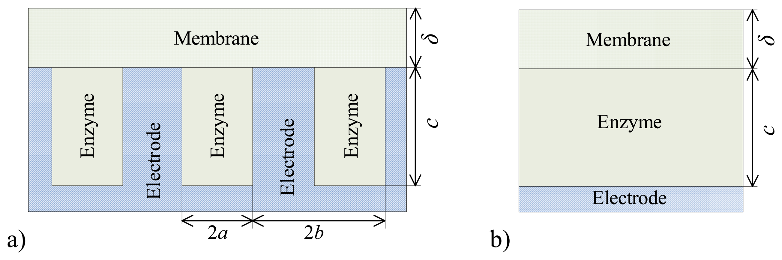
De and the following values of the domain geometry: b = 2a = 4μm, c = 4μm, d = c + δ. In the case of the plate–gap biosensor the geometry parameter c stands for the depth of the gaps while in the case of the flat biosensor it stands for the thickness of the enzyme layer. Of course, a and b are vacuous for the flat biosensors. 
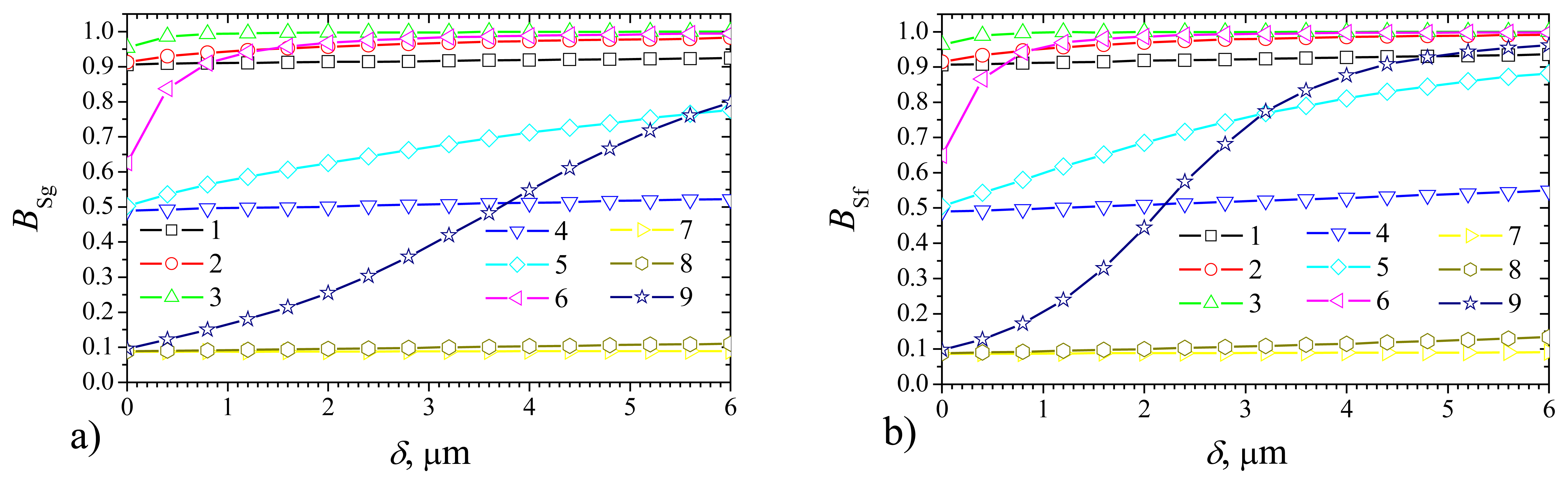
Fig. 4 shows the effect of the membrane thickness δ on the biosensor sensitivity at the same values of the parameters as in Fig. 3.
One can see in Fig. 3, that the shape of the normalized steady state currents Iδg and Iδf (as well as of the non–normalized ones Ig and If) is very sensitive to changes of the maximal enzymatic rate Vmax and substrate concentration S0. Iδg and Iδf are monotonous decreasing functions of the outer membrane thickness δ at a high value of Vmax (10 mM/s) and relatively low values of S0 (0.1 and 1 mM) (curves 3 and 6). Iδg and Iδf are monotonous increasing functions of δ at low enough values of Vmax (0.1 and 1.0 mM/s) and a high value of S0 (10 mM) (curves 7 and 8).
Very similar behavior of the biosensor response was observed when modeling one–layer biosensors acting in a non–stirred analyte [24]. Then the steady state biosensor current was found to be a monotonous decreasing function of the thickness of the external diffusion layer if the biosensor response is distinctly under diffusion control (σ2 > 1). In the cases when the enzyme kinetics controls the biosensor response (σ2 < 1), the steady state current increases with increase of the thickness of the diffusion layer. Thus the steady state current varied up to several times. When σ2 ≈ 1, the variation of the steady state current is rather small. Let us notice that in the cases presented in Fig. 3, σ2 = 0.16 at Vmax = 0.1 mM/s and σ2 = 1.6 at Vmax = 10 mM/s.
When comparing simulation results of biosensors of different types, we can see in Fig. 3 that the response of the flat biosensor may increase by a factor of about 1.9 times when changing δ, while the corresponding factor for the plate–gap biosensor equals only about 1.15. Consequently, at low maximal enzymatic rates and high substrate concentrations (S0 > KM) the response of the plate–gap biosensor is more stable to changes of the thickness δ of the outer membrane than the response of the flat one.
As one can see in Fig. 4, the effect of the thickness δ of the outer membrane on the sensitivity of the plate–gap biosensor is very similar to that of the flat one. Fig. 4 shows well known feature of biosensors, that the biosensor sensitivity is higher at lower substrate concentrations rather than at higher ones. However, in the cases of high enough enzymatic activity, the sensitivity can be notably increased by increasing the thickness δ of the outer membrane even at high substrate concentrations (curves 5, 6, 9 in Fig. 4). Thus, the advantage of the outer membranes to prolong the region of the application of the biosensor is applicable also to gap–plate biosensors not only to flat ones [1012].
On the other hand, at high values of Vmax and S0 (curve 9), the sensitivity of the plate–gap biosensor (Fig. 4a) is slightly more stable than of the flat one (Fig. 4b) to changes in the thickness δ. This feature increases the reliability of a bioanalytical system which is one of the most important parameters of biosensors. This feature is very important in the biosensors implanted into systems with unstable pressure (body blood system, or reactor with peristaltic pumping of the probe). Fluctuations of the outer membrane of the biosensor induced by fluctuations of the pressure can influence distance of the diffusion way, thereby influence response of the biosensor.
The main physical reason of the superior behavior of the plate–gap biosensors vs. the flat ones is that the product of the enzymatic reaction is better (more completely) converted into the biosensor current. The product, which is electro–active substance, is better captured, i.e. it has less time to diffuse away before it is electro–oxidized or – reduced, in the plate–gap model rather than in flat one.
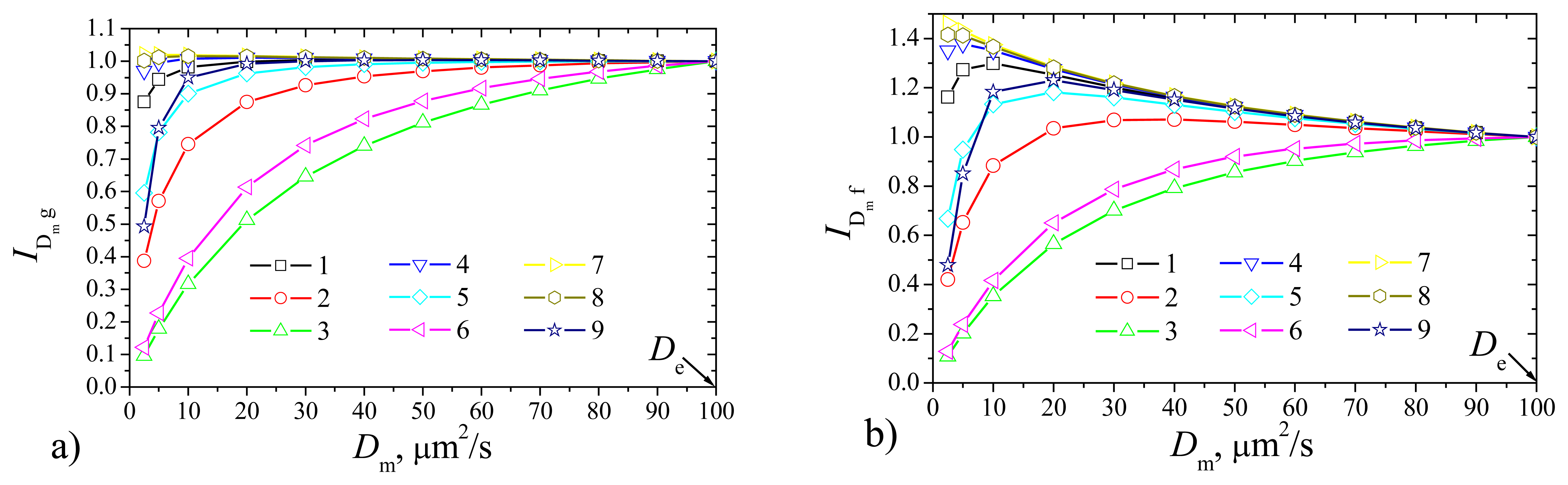
To investigate the dependence of the biosensor response on the diffusivity Dm = DSm = DPm of the outer membrane the biosensor responses were calculated at constant thickness δ = 2 μm of the outer membrane changing the diffusion coefficient Dm from 1 to 0.025 μm2/s, i.e. from De to 1/50 De. In this case the current was normalized with respect to the maximal value De of the diffusivity the outer membrane to be analyzed,
I D m α ( D m ) = I α ( D m ) I α ( D e ) , α = f ,
where If(Dm) and Ig(Dm) are the steady state currents calculated at the diffusivity Dm the outer membrane for the flat and plate–gap biosensors, respectively. Results of the calculations are depicted in Fig. 5, where one can see, that the effect of the diffusivity Dm notably depends on the maximal enzymatic rate Vmax and substrate concentration S0. Although the shapes of curves in Fig. 5 notable differ from those in Fig. 3, the effect of the diffusivity Dm of the membrane is very similar to that of the membrane thickness δ. A decrease in diffusivity influences the steady state current similarly to the increase in thickness of the membrane. The plate–gap biosensor is notably less sensitive to changes of the permeability of the outer membrane than the corresponding flat biosensor. However, this peculiarity is valid only in the cases when the biosensor operates at low maximal enzymatic rates and high substrate concentrations (S0 > KM) conditions.
The similarity between the effects of the outer membrane thickness δ on the biosensor response and that of the diffusivity Dm is also notable when comparing Figs. 4 and 6. Particularly, in the cases of high enough enzymatic activity and high substrate concentrations the sensitivity can be significantly increased by decreasing the diffusivity Dm of the outer membrane (curves 5, 6, 9 in Fig. 6).
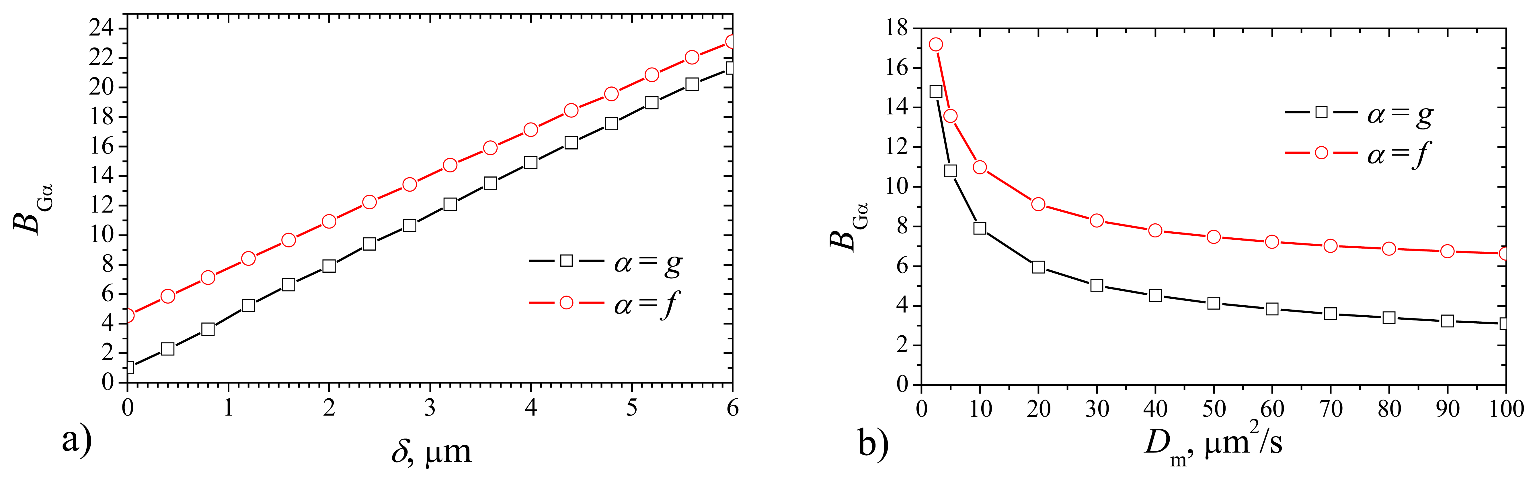
When calculating the maximal gradients BGg and BGf of the biosensor responses, no notable difference was found changing the substrate concentration S0 and maximal enzymatic rate Vmax. Changing S0 and Vmax in several orders of magnitude, values of the gradients BGg and BGf varied less than 1%. However, the effect of the thickness δ as well as of the diffusivity Dm of the outer membrane on the biosensor response was substantial. As one can see in Fig. 7, the maximal gradient increases with increase of the thickness δ as well as with decrease of the diffusivity Dm. However, the shape of curves differs. The maximal gradient is practically linear function of δ, while it is highly non linear monotonously decreasing function of Dm. The maximal gradient method of evaluation of biosensor response usually is used in bioanalytical instruments, when the time of the measurement cycle is necessary to reduce, thereby, to increase the speed of the analysis. Another feature – after the biosensor response passes maximal gradient, probe can be removed or replaced by buffer, and thereby the biosensor operates at lower concentrations of the substrate inside of the membrane and products as well. In some cases it is important for the stability of the biosensor, because the product of the enzymatic reaction can be chemically active and destroy the membrane (for example, a number of biosensors, containing oxidases and producing hydrogen peroxide;. This positive feature compensates the worse stability of biosensor concerning the sensitivity to the fluctuations of the membrane thickness.
Fig. 7 shows that the absolute difference between the gradients of different biosensors varies slightly, 1.8 < BGfBGg < 3.6. The maximal gradient of the response of plate–gap biosensor is lower than that of the corresponding flat one. Additional numerical experiments at other values of the parameters approved this feature. This can be explained by difference in the geometry of the electrodes. When the enzyme reaction starts, the gradient of the current gains the maximum immediately after some product touches the electrode surface, i.e. at the very beginning of the biosensor operation. The delay time depends mainly on the rate of the diffusion through the enzyme. In the case of the flat biosensor the touch occurs in one time at entire surface of the electrode, while in the case of the plate–gap biosensor, the current arises very gradually: firstly on the sides of gaps (from outside to inside the biosensor) and only then on the bottom of gaps. The current gradient is greater when the current arises like avalanche, i.e. in the case of the flat biosensor.

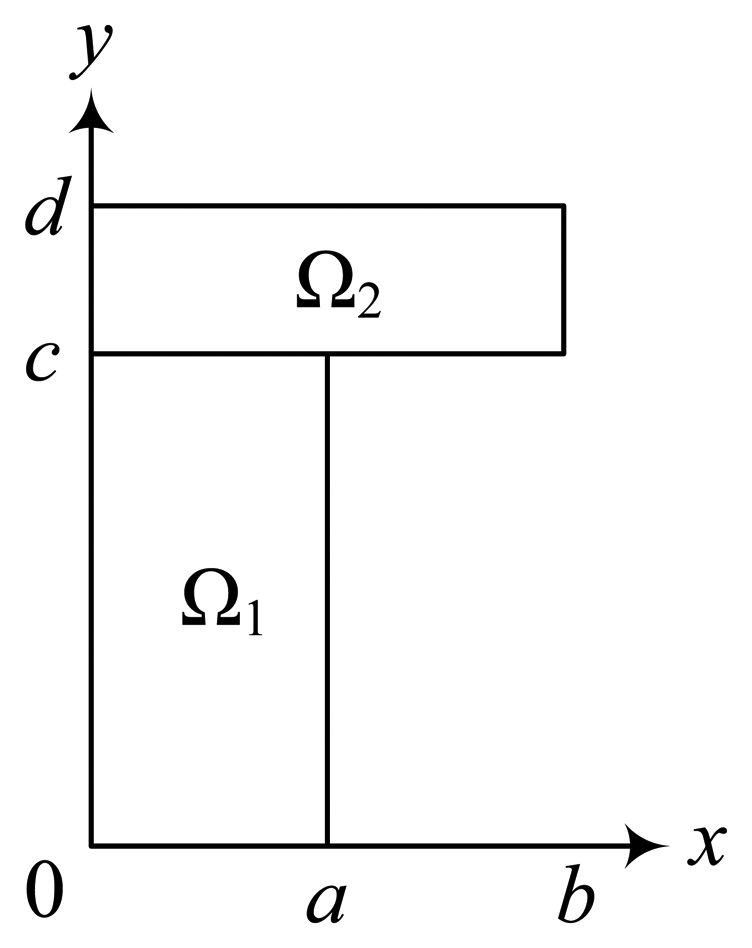
5.2. The Effect of the Geometry of Gaps on the Biosensor Response

For the plate–gap biosensors the model parameter c (Fig. 1a) stands for the depth of the gaps in the electrode. In the case of the corresponding flat biosensors (Fig. 1b) c is the thickness of the enzyme layer. Fig. 8 shows the dependence of the steady state biosensor current on the parameter c, while Fig. 9 shows the dependence of the biosensor sensitivity on that parameter. The biosensors responses were calculated at constant thickness δ = 2μm and constant diffusivity Dm = 0.1μm2/s of the outer membrane changing c from 2 to 6 μm. In this case the steady state currents were normalized with respect to the minimal value c0 of c to be analyzed,
I c α ( c ) = I α ( c ) I α ( c 0 ) , α = f , g ,
where If(c) and Ig(c) are the steady state currents calculated at a value c, c0 = 2 μm.
As it is possible to notice in Fig. 8, the effect of the depth of the gaps on the steady state current (Fig. 8a) is very similar to that of the thickness of the enzyme layer (Fig. 8b). The steady state current of the plate–gap biosensor as well as of the flat one are monotonous increasing functions of c. However, Icg and Icf are practically constant functions of c at high maximal enzymatic rate Vmax (10 mM/s) and relatively low values of S0 (0.1 and 1 mM) (curves 3 and 6).
Let us notice, that these properties are valid at values of c specific to the plate–gap biosensors, i.e. when the depth of gaps is of a few micrometers. At wide range of c it may not be true, e.g. in the case of biosensors with a mono–enzyme layer, the steady state current is a non–monotonous function of the thickness of the enzyme layer [17].
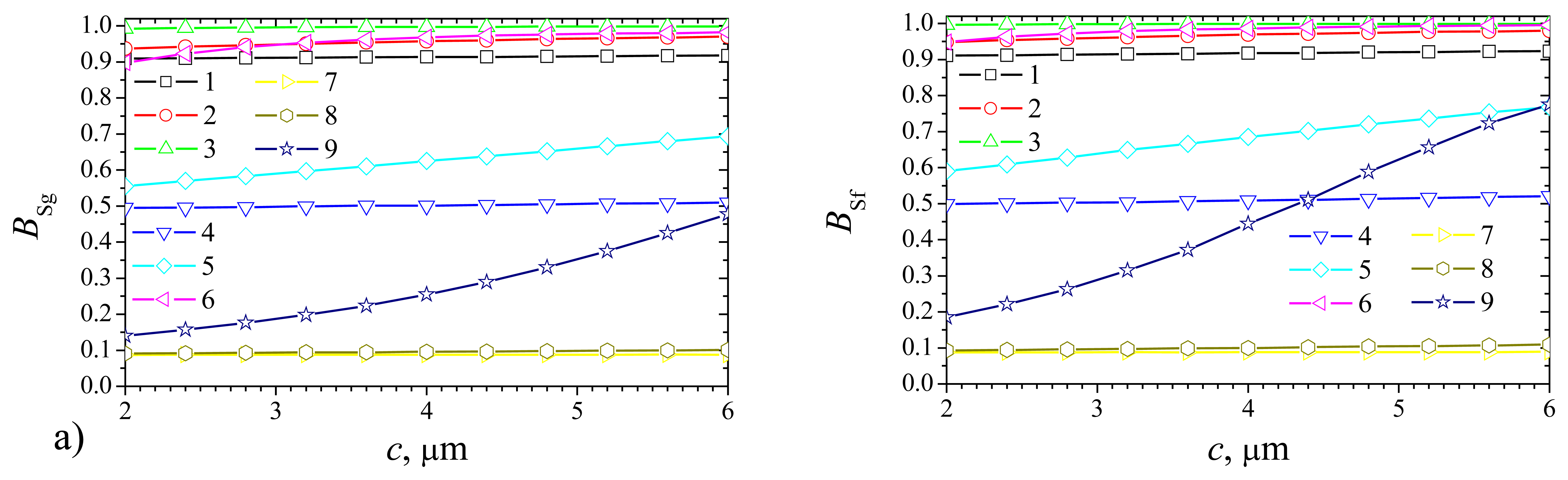
Fig. 9 shows that the effect of the gap depth on the sensitivity of the plate–gap biosensor is very similar to that of the thickness of the enzyme layer of the flat biosensor. However, it is possible to notice, that the sensitivity of the plate–gap biosensor (Fig. 9a) is slightly more stable than of the flat one (Fig. 9b) to changes in c only at very high values of Vmax and S0 (curve 9).
To investigate the dependence of the biosensor response on the width of the gaps we calculated the biosensor response at a constant distance 2(ba) between two adjacent gaps changing the half width a from to 0.5μm to 5 μm. As it was mentioned above, increasing the half width a of the gaps the current density of the plate–gap biosensor approaches the current density of the corresponding flat one, i.e. IgIf when a → ∞. Because of this the steady state currents of the plate–gap biosensor were normalized with the steady state current of the corresponding flat biosensor,
I ag ( a ) = I g ( a ) I f , lim a I g ( a ) = I f , lim a I ag ( a ) = 1 ,
where Ig(a) is the steady state current calculated assuming the width a of the gaps, and If is the steady state current of the corresponding flat biosensor. Fig. 10a shows the dependence of the steady state current of the plat–gap biosensor on the width a of the gaps at different values of Vmax and S0. As one can see in Fig 10a, the Iag(a) approaches to unit rather quickly. At a = 1.5b = 3μm the relative difference between Ig(a) and If does not exceed 20% (Iag0.8). At very high maximal enzymatic rate Vmax (10 mM/s) and low values of the concentration S0 (0.1 and 1 mM) (curves 3 and 6) Ig(a) approaches If notable faster than at other values of Vmax and S0.
An increase in the width as well as in the depth of the gaps increases the volume of the enzyme used in plate–gap biosensors. Summarizing the results presented in Figs. 8, 9 and 10a, we can notice, that the biosensors of two considered types: plate–gap and flat, both with the outer membrane, are more resistant to changes in volume of the enzyme at lower values of Vmax rather than at higher ones and at higher values of S0 rather than at lower ones.
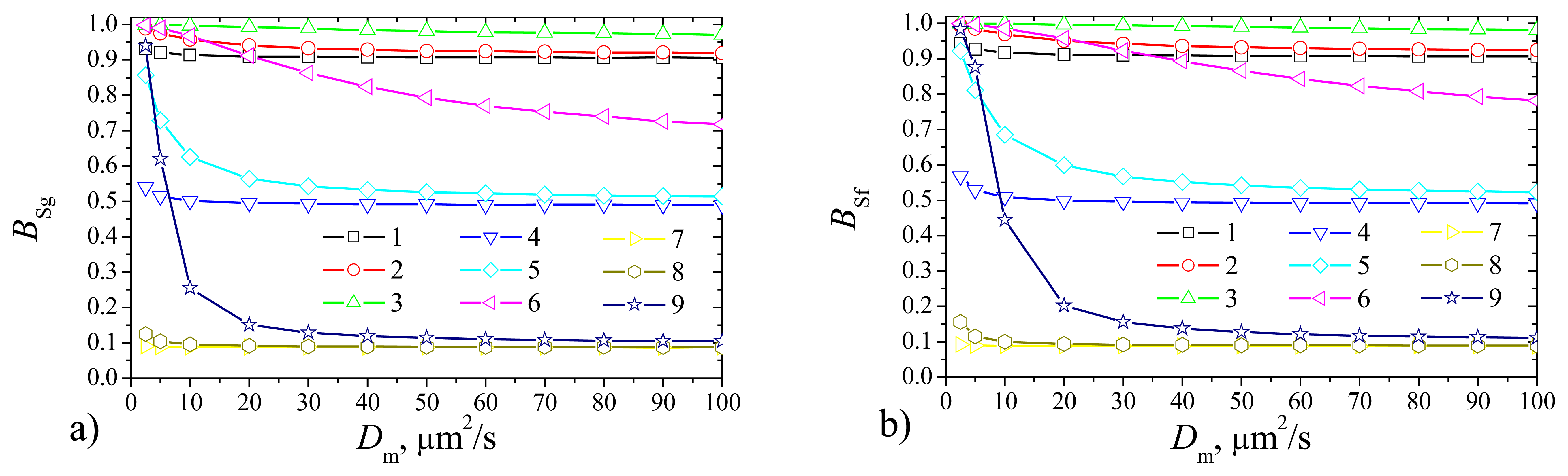
Fig. 10b shows the dependence of the sensitivity BSg of the plate–gap biosensor on the width of the gaps. As it is possible to notice in Fig. 10b the sensitivity BSg is practically constant function of the width a of the gaps when a varies from 0.5 to 5μm. Fig. 10b shows also an important influence of the substrate concentration S0 upon the biosensor sensitivity BSg. At all the values of a the lower concentration S0 corresponds to the higher sensitivity BSg. This feature of the biosensor is very well known [13,17]. The effect of the maximal enzymatic rate Vmax on the biosensor sensitivity is more or less notable only in the cases when the substrate concentration S0 varies about the Michaelis constant KM, i.e. when the enzyme kinetics changes from zero order to the first order across the enzyme region, S0KM.

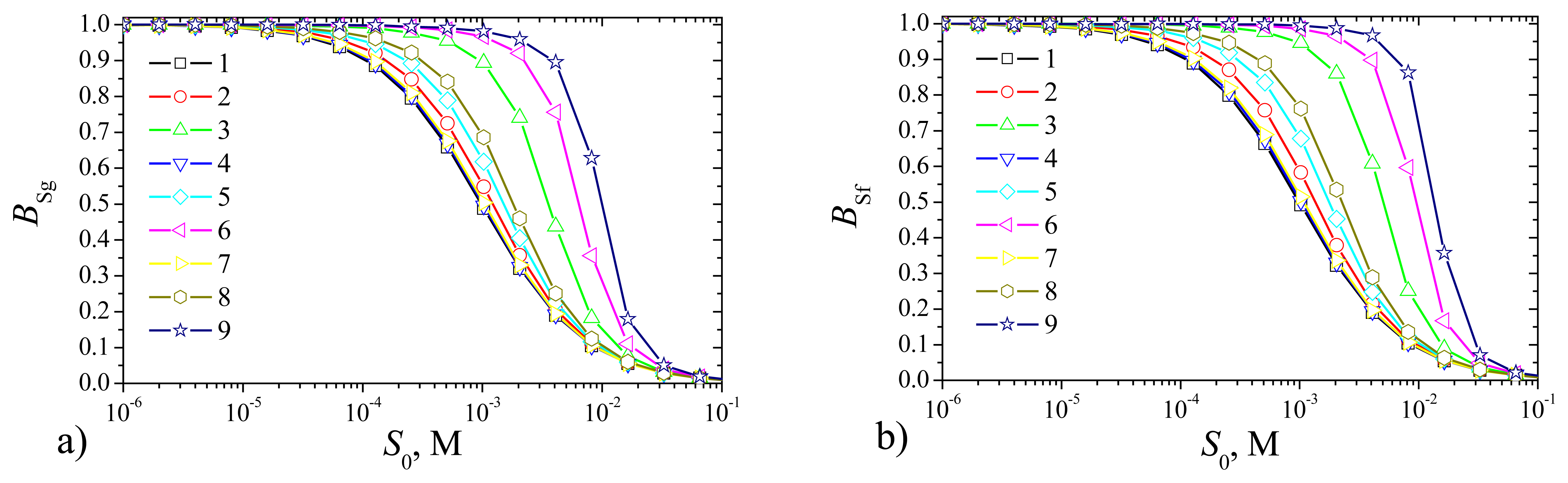
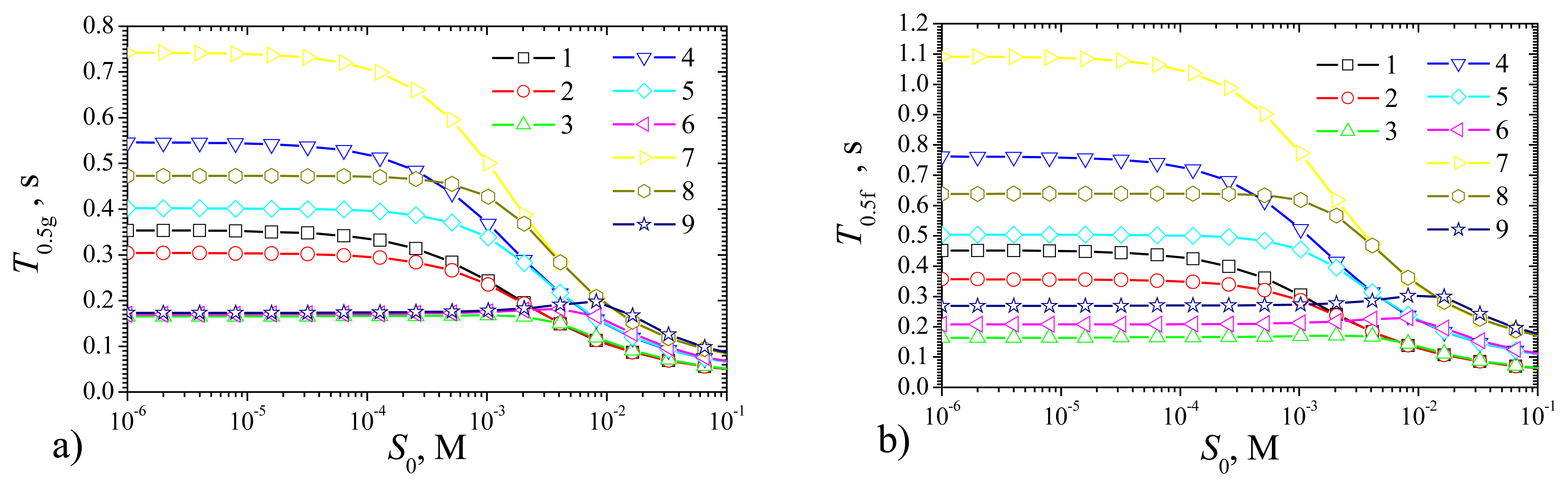
5.3. The Dependence of the Biosensor Response on the Substrate Concentration

To investigate the dependence of the biosensor response on the substrate concentration the response was simulated at wide range of the concentrations S0. Fig. 11 shows the steady state currents, Fig. 12 shows the sensitivities, and Fig. 13 shows the half times of the steady state for both types of biosensors: the plate–gap and the flat.
As one can see in Fig. 11 the density Ig of the steady state current of the plate–gap biosensor is slightly less than that of the flat one. However, when comparing the simulation results of the biosensors of different types one can see very similar shape of all curves. Very similar shapes of all curves we can see also in Fig. 12 presenting the sensitivity of the biosensors at the same values of the parameters as in Fig. 11. Thus, the recognition capability of the novel plat–gap biosensors is very similar to the corresponding flat biosensors both with the outer membranes.
As it is possible to notice in Fig. 13, T0.5g and T0.5f are monotonous decreasing functions of S0 at the maximal enzymatic rate Vmax of 10 as well as of 100 mM/s. At S0 being between 0.1 and 10 mM (between KM and 100 KM) shoulders on the curves appears for Vmax = 1 mM/s. It seems possible that the shoulders on the curves arise because of high maximal enzymatic rate Vmax at the substrate concentrations at which the kinetics changes from zero order to first order across the enzyme region. At substrate concentration S0KM the reaction kinetics for S is zero order throughout the enzyme region whereas for S0KM the kinetics is first order throughout. At intermediate values of S0 the kinetics changes from zero order to first order across the membrane. Similar effect of the substrate concentration on the response time was noticed in the cases of an amperometric biosensor based on an array of enzyme microreactors [21] and of the oxidation of β-nicotinamide adenine dinucleotide (NADH) at poly(aniline;-coated electrodes [30]. Fig. 13 shows that at high substrate concentration S0 = 100 mM (S0 = 100 KM), the catalytic reaction makes no notable effect on the biosensors response time.

6. Conclusions

The mathematical model (3)(9) can be successfully used to investigate regularities of the response of the plate–gap biosensors with the porous outer membrane (Fig. 1a).
At low maximal enzymatic rates (Vmax) and high substrate concentrations (S0 > KM) the response of the plate–gap biosensor is more resistant to changes of the thickness of the outer membrane than the response of the corresponding flat one (Fig. 3). At these conditions, the steady state current of the plate–gap biosensor is also more resistant to changes in the permeability (the diffusivity) of the outer membrane than the corresponding flat electrode deposited with a layer of enzyme and covered with the same inert membrane (Fig. 5). These features of the biosensor are very important for long–term operating analytical systems when activity of the enzyme in the membrane decreases and the outer surface of the biosensor is glued with proteins and other components of the probe.
The response of the biosensors of two considered types: plate–gap and flat, both with the outer membrane, is more resistant to changes in volume of the enzyme at lower values of Vmax rather than at higher ones and at higher values of S0 rather than at lower ones (Fig. 8, 10a). The sensitivity of the biosensors of both types is very similar (Fig. 9). These features of the biosensors can be applied in design of novel highly sensitive biosensors when the minimization of the enzyme volume is of crucial importance. Selecting the geometry of gaps allows minimizing the volume of enzyme without loosing the sensitivity.
The maximal gradient of the current of plate–gap biosensor is lower than that of the corresponding flat one. In both cases, the maximal gradient is practically linear increasing function of thickness of the outer membrane and it is non linear monotonously decreasing function of the diffusivity of the membrane (Fig. 7).
Work is now in progress to compare the simulations obtained for plate–gap biosensors with similar experimental studies [31].

Acknowledgments

This work was partially supported by Lithuanian State Science and Studies Foundation, project No. C–03048.

References

  1. Clarc, L. C.; Loys, C. Electrode system for continuous monitoring in cardiovascular surgery. Ann. N.Y. Acad. Sci. 1962, 102, 29–45. [Google Scholar]
  2. Scheller, F.; Schubert, F. Biosensors; Vol. 7, Amsterdam; Elsevier, 1988. [Google Scholar]
  3. Turner, A.P.F.; Karube, I.; Wilson, G.S. Biosensors: Fundamentals and Applications; Oxford University Press: Oxford, 1987. [Google Scholar]
  4. Chaubey, A.; Malhotra, B.D. Mediated biosensors. Biosens. Bioelectron. 2002, 17, 441–456. [Google Scholar]
  5. Rogers, K.R. Biosensors for environmental applications. Biosens. Bioelectron. 1995, 10, 533–541. [Google Scholar]
  6. Wollenberger, U.; Lisdat, F.; Scheller, F.W. Frontiers in Biosensorics 2. Practical Applications; Birkhauser Verlag: Basel, 1997. [Google Scholar]
  7. Fraser, D.M. (Ed.) Biosensors in the Body: Continuous in vivo Monitoring; John Wiley & Sons: Chichester, 1997.
  8. Treloar, P.H.; Christie, I.M.; Vadgama, P.M. Engineering the right membranes for electrodes at the biological interface; solvent cast and electropolymerised. Biosens. Bioelectron. 1995, 10, 195–201. [Google Scholar]
  9. Antiochia, R.; Lavagnini, I.; Magno, F. Amperometric mediated carbon nanotube paste biosensor for fructose determination. Anal. Let. 2004, 37, 1657–1669. [Google Scholar]
  10. Schöning, M.J. “Playing around” with field-effect sensors on the basis of EIS structures, LAPS and ISFETs. Sensors 2005, 5, 126–138. [Google Scholar]
  11. Laurinavicius, V.A.; Kulys, J.J.; Gureviciene, V.V.; Simonavicius, K.J. Flow–through and cateter biosensors with an extended concentration range. Biomed. Biochem. Acta. 1989, 48, 905–909. [Google Scholar]
  12. Lyons, M.E.G.; Murphy, J.; Rebouillat, S. Theoretical analysis of time dependent diffusion, reaction and electromigration in membranes. J. Solid State Electrochem. 2000, 4, 458–472. [Google Scholar]
  13. Kulys, J. The development of new analytical systems based on biocatalysts. Anal. Lett. 1981, 14, 377–397. [Google Scholar]
  14. Schulmeister, T. Mathematical treatment of concentration profiles and anodic current of amperometric enzyme electrodes with chemically–amplified response. Anal. Chim. Acta 1987, 201, 305–310. [Google Scholar]
  15. Bartlett, P.N.; Pratt, K.F.E. Modelling of processes in enzyme electrodes. Biosens. Bioelectron. 1993, 8, 451–462. [Google Scholar]
  16. Sorochinskii, V.V.; Kurganov, B.I. Steady–state kinetics of cyclic conversions of substrate in amperometric bienzyme sensors. Biosens. Bioelectron. 1996, 11, 225–238. [Google Scholar]
  17. Baronas, R.; Ivanauskas, F.; Kulys, J. The influence of the enzyme membrane thickness on the response of amperometric biosensors. Sensors 2003, 3, 248–262. [Google Scholar]
  18. Ivanauskas, F.; Kaunietis, I.; Laurinavicius, V.; Razumiene, J.; Simkus, R. Computer simulation of the steady state currents at enzyme doped carbon paste electrode. J. Math. Chem. 2005, 38, 355–366. [Google Scholar]
  19. Schulmeister, T. Mathematical modeling of the dynamic behaviour of amperometric enzyme electrodes. Selective Electrode Rev. 1990, 12, 203–206. [Google Scholar]
  20. Baronas, R.; Ivanauskas, F.; Survila, A. Simulation of electrochemical behavior of partially blocked electrodes under linear potential sweep conditions. J. Math. Chem. 2000, 27, 267–278. [Google Scholar]
  21. Baronas, R.; Ivanauskas, F.; Kulys, J. Mathematical modeling of biosensors based on an array of enzyme microreactors. Sensors 2006, 6, 453–465. [Google Scholar]
  22. Bakhvalov, N.S.; Panasenko, G.P. Homogenization: Averaging Processes in Periodic Media; Dordrecht; Kluwer Academic Publishers, 1989. [Google Scholar]
  23. Schulmeister, T.; Pfeiffer, D. Mathematical modelling of amperometric enzyme electrodes with perforated membranes. Biosens. Bioelectron. 1993, 8, 75–79. [Google Scholar]
  24. Baronas, R.; Ivanauskas, F.; Kulys, J. Computer simulation of the response of amperometric biosensors in stirred and non stirred solution. Nonlinear Anal. Model. Control 2003, 8, 3–18. [Google Scholar]
  25. Britz, D. Digital Simulation in Electrochemistry, 2nd ed.; Berlin; Springer–Verlag, 1988. [Google Scholar]
  26. Bieniasz, L.K.; Britz, D. Recent developments in digital simulation of electroanalytical experiments. Polish J. Chem. 2004, 78, 1195–1219. [Google Scholar]
  27. Samarskii, A.A. The Theory of Difference Schemes; New York–Basel; Marcel Dekker, 2001. [Google Scholar]
  28. Moreira, J.E.; Midkiff, S.P.; Gupta, M.; Artigas, P.V.; Snir, M.; Lawrence, R.D. Java programming for high performance numerical computing. IBM Systems J. 2000, 39, 21–56. [Google Scholar]
  29. Crank, J. The Mathematics of Diffusion, 2nd ed.; Oxford; Clarendon Press, 1975. [Google Scholar]
  30. Bartlett, P.N.; Birkin, P.R.; Wallace, E.N.K. Oxidation of β-nicotinamide adenine dinucleotide (NADH) at poly(aniline)-coated electrodes. J. Chem. Soc. Faraday Trans. 1997, 93, 1951–1960. [Google Scholar]
  31. Laurinavicius, V.; Razumiene, J.; Ramanavicius, A.; Ryabov, A.D. Wiring of PQQ-dehydrogenases. Biosens. Bioelectron. 2004, 20, 1217–1222. [Google Scholar]
Figure 1. A principal structure of a plate–gap biosensor (a) and the corresponding flat one (b), both with the outer membrane. The figure is not to scale.
Sensors 06 00727f1
Figure 2. A profile of the unit cell of the plate–gap biosensor.
Sensors 06 00727f2
Figure 3. The normalized steady state current vs. the thickness δ of the outer membrane in the cases of plate–gap (a) and flat (b) biosensors at three maximal enzymatic rates Vmax: 0.1 (1, 4, 7), 1 (2, 5, 8), 10 (3, 6, 9) mM/s and three substrate concentrations S0: 0.1 (1–3), 1 (4–6), 10 (7–9) mM, Dm = 0.1μm2/s, b = 2a = 4μm, c = 4μm, d = c + δ.
Sensors 06 00727f3
Figure 4. The normalized biosensor sensitivity vs. the thickness δ of the outer membrane in the cases of plate–gap (a) and flat (b) biosensors. The parameters and notations are the same as in Fig. 3.
Sensors 06 00727f4
Figure 5. The normalized steady state current vs. the diffusivity Dm of the outer membrane in the cases of plate–gap (a) and flat (b) biosensors at the thickness δ = 2 μm of the outer membrane. Other parameters and the notations are the same as in Fig. 3.
Sensors 06 00727f5
Figure 6. The normalized biosensor sensitivity vs. the diffusivity Dm of the outer membrane in the cases of plate–gap (a) and flat (b) biosensors, δ = 2 μm, other parameters are the same as in Fig. 3.
Sensors 06 00727f6
Figure 7. The normalized maximal gradient vs. the thickness δ (a) and the diffusivity Dm (b) of the outer membrane, Vmax = 1 mM/s, S0 = 1 mM/s, Dm = 0.1μm2/s (a), δ = 2 μm (b), other parameters are the same as in Fig. 3.
Sensors 06 00727f7
Figure 8. The normalized steady state current vs. the gap depth c of the plate–gap biosensor (a) and the thickness of enzyme layer of the flat one (b), δ = 2 μm. Other parameters and the notations are the same as in Fig. 3.
Sensors 06 00727f8
Figure 9. The normalized biosensor sensitivity vs. the gap depth c of the plate–gap biosensor (a) and the thickness of enzyme layer of the flat one (b), δ = 2 μm. Other parameters and the notations are the same as in Fig. 3.
Sensors 06 00727f9
Figure 10. The normalized steady state current (a) and the biosensor sensitivity (b) vs. the gap width a of the plate–gap biosensor, δ = 2 μm, b = a+2 μm. Other parameters and the notations are the same as in Fig. 3.
Sensors 06 00727f10
Figure 11. The steady state current vs. the substrate concentration S0 in the cases of plate–gap (a) and flat (b) biosensors at three maximal enzymatic rates Vmax: 0.1 (1, 4, 7), 1 (2, 5, 8), 10 (3, 6. 9) mM/s and three values of c: 2 (1–3), 4 (4–6), 6 (7–9) μm, Dm = 0.1μm2/s, b = 2a = 4μm, c = 4μm, δ = 2μm.
Sensors 06 00727f11
Figure 12. The normalized biosensor sensitivity vs. the substrate concentration S0 in the cases of plate–gap (a) and flat (b) biosensors. The parameters and notations are the same as in Fig. 11.
Sensors 06 00727f12
Figure 13. The half time of the steady state biosensor response vs. the substrate concentration S0 in the cases of plate–gap (a) and flat (b) biosensors. The parameters and notations are the same as in Fig. 11.
Sensors 06 00727f13

