1. Introduction
The need for low-power, miniature sensor devices that can monitor air quality in an enclosed space with multi-compound capability and minimum human operation prompts the development of polymer-based electronic nose (ENose) at NASA's Jet Propulsion Laboratory (JPL) and California Institute of Technology [
1-
3]. The sensor array in the ENose, which was recently built at JPL and demonstrated aboard NASA's space shuttle flight STS-95, consists of 32 conductometric sensors made from insulating polymer films loaded with carbon. In its current design, it has the capability to detect 10 common contaminants which may be released into the recirculated breathing air of the space shuttle or space station from a spill or a leak; target concentrations are based on the 1-hour Spacecraft Maximum Allowable Concentrations (SMAC) set by NASA (see Table I) [
4], and are in the parts-per-million (ppm) range. In addition, the device can detect changes in humidity and a marker analyte described in Section 4. The ENose was intended to fill the gap between an alarm which sounds at the presence of chemical compounds but with little or no ability to distinguish among them, and an analytical instrument which can distinguish all compounds present but with no real-time or continuous event monitoring ability.
The specific analysis scenario considered for this development effort was one of leaks or spills of specific compounds. It has been shown in analysis of samples taken from space shuttle flights that, in general, air is kept clean by the air revitalization system and contaminants are present at levels significantly lower than the SMACs [
5]; this device has been developed to detect target compounds released suddenly into the environment. A leak or a spill of a solvent or other compound would be an unusual event. Release of mixtures of more than two or three compounds would be still more unusual; such an event would require simultaneous leaks or spills to occur from separate sources. Thus, for this phase of development, mixtures of more than two target analytes were not considered.
As in other array-based sensor devices, the individual sensor films of the ENose are not specific to any one analyte; it is in the use of an array of different sensor films that gases or gas mixtures can be uniquely identified by the pattern of measured response. The response pattern requires software analysis to identify the compounds and concentrations causing the response. The primary goal in analysis software development was to identify events of single or mixed gases from the 10 target compounds plus humidity changes and marker analyte with at least 80% accuracy (fewer than 20% false positives and false negatives) in both identification and quantification, where accurate quantification is defined as being +/−50% of the known concentration. Correct identification of the compound causing a test event with quantification outside the +/-50% range is considered to be a false positive. Failure to detect an event is a false negative. The rather tolerant quantification range was defined by the Toxicology Branch at NASA-Johnson Space Center (NASA-JSC) and reflects the fact that the SMACs are defined in a similar way: the toxic level of most of the compounds is not known more accurately than +/(− 50%, so the SMACs have been set at the lower end [
5].
Many data analysis methods are available for this purpose, including some well studied statistical methods and their variations, such as Principal Component Analysis, Discriminant Function, Multiple Linear Regression, and Partial Least Squares [
6-
11]. In addition, there are more recent neural network based approaches, particularly multilayer neural networks with back propagation [
6,
12-
16]. The choice of an appropriate data analysis method for sensor chemophysics (odor detection/classification) is, however, often highly dependent on the nature of the data, the application scenarios, and analysis objectives for the specified application. To date, polymer-based sensor arrays have been used mostly in fairly restricted application scenarios. Air quality monitoring with the JPL ENose is a challenging task, consisting of a large number of target analytes in a partially controlled atmosphere. Target analytes may be present as single gases or as mixtures of those gases. In addition, the task requires quantification of detected analytes as well as the capability for future implementation of autonomous quasi real time analysis. There were twelve target compounds in this phase, and there will be 20-30 in the next phase; binary mixtures were studied in this work, and mixtures of up to 4 compounds will be studied in the future. In addition to these requirements, we also faced challenging conditions such as large variation in some of the response patterns, analytes of similar chemical structure and hence of similar (correlated) signature patterns, and limited data available for mixtures during the algorithm development. Data sets of sensor array response were taken in parallel with algorithm development because of time constraints, but the data analysis goal was to be prepared to deconvolute any potential mixtures for the flight experiment. A series of software routines was developed using MATLAB as a programming tool. Several different approaches were considered and investigated in the process. Eventually a modified Levenberg-Marquardt nonlinear least squares based method was developed and its effectiveness demonstrated amid highly noisy and nonlinear responses from the ENose sensor array.
2. Development of data analysis approach
During the early stages of the analysis software development, three conceptually different approaches to ENose data analysis were developed in parallel: Discriminant Function Analysis (DFA), Neural Networks with Back Propagation (NNBP), and a Linear Algebra (LA) based approach [
2]. Principal Component Analysis (PCA) was used initially, but was later replaced by DFA (Fisher Discriminant) because of its superior ability to discriminate similar signatures that contain subtle, but possibly crucial, gas-discriminatory information. Both DFA and NNBP are among the popular methods for array-based sensor data analysis. In general, NNBP is more suitable than DFA when the sensor signatures of two gases are not separable by a hyperplane (e.g., one gas has a signature surrounding the signature of another gas), while DFA is better in classifying data sets which may overlap. Both DFA and NNBP were developed primarily for identifying single gases. The quantification was then obtained by its overall resistance change strength using pre-calibrated data.
The main reason to develop a LA based approach is that neither DFA nor NNBP were found to be well suited for resolving signatures resulting from a combination of more than one gas compound. Very little training data were available on mixtures during much of the time the algorithm was under development, and limited data were available later; nevertheless, the software was required to be ready to deconvolute potential mixtures for the flight experiment. Consequently we chose to use a LA based approach, which enables us to find the best solution among many possible solutions by limiting the non-zero elements in deposition and choosing the one with the sparsest possible significant elements.
In a LA based method one tries to solve the equation
y=Ax, where vector
y is an observation (a response pattern), vector
x is the cause for the observation (concentrations of a gas or combinations of gases), and matrix
A describes system characteristics (gas signatures obtained from training data). Since we have more sensors than target compounds and the response pattern is often noise corrupted, both of which mean there may exist no exact solution, the least-squares method is the most appropriate way to solve the equation [
17,
18]. We obtained the best solution in the least squares sense as
x=A+y, where
A+=Q2D+Q1T is the pseudoinverse by Singular Value Decomposition (SVD) of
A (i.e.,
A=Q1DQ2T),
Q1 and
Q2 are orthogonal and
D is diagonal.
D+ is found from
D by inverting all nonzero elements. We solve the equation under the constraint that
n out of
N (
N=10) components of
x are equal to 0; we then examine each of these solutions (total 225 for
n=5) and select the one with the fewest nonzero and nonnegative elements, as in the expected scenario of anomalous event detection we expect fewer rather than more different compounds to appear.
It should be noted that the LA based method requires that the sensors follow linearity and additive linearity (superposition) properties,
i.e. the response to a mixture of compounds is a linear combination of the response to the individual compounds; these properties were shown in previous studies on similar sensor sets [
19-
21]. Compared to methods that use concentration-normalized sensor response to identify unknown gas(es) first, by using PCA, for example, and then determine concentration(s) from previously calibrated data by a second analysis, such as Multiple Linear Regression (MLR), Partial Least Squares (PLS), or Principal Component Regression (PCR) [
7], the LA based method effectively combines the two steps of identification and quantification into one. This combination helps to facilitate the automation of data analysis without human intervention.
The idea of developing three parallel methods is that one can first use the LA method to deconvolute an unknown response pattern as a linear combination of target compounds; unknown compounds were expressed as a combination of four compounds or fewer. If a single compound is found, additional verification can be then carried out by NNBP and DFA methods to improve the identification success rate [
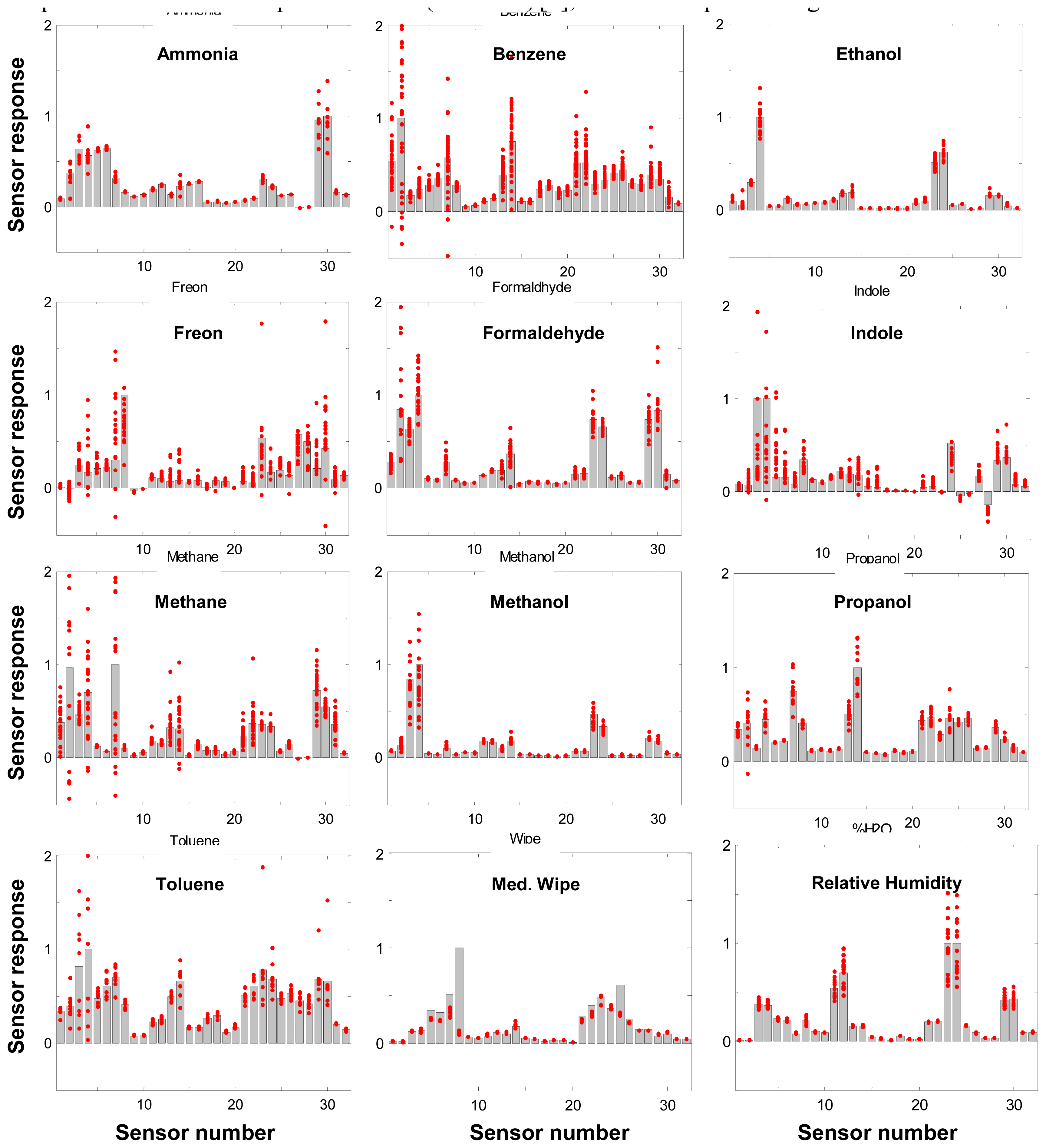
2]. In the course of the work we found that, even for single gases, the LA method performed consistently best among the three, while DFA was consistently the worst. The average success rates using DFA, NNBP, and LA methods for singles in the early stages of development were 35%, 50% and 60%, respectively. The poor performances of DFA and NNBP are due largely to poor repeatability of responses of the ENose sensor array (noisy fingerprints, see
Figure 1), which, as with most polymer-based sensors, is sensitive to temperature, humidity, pressure, air flow, sensor saturation and aging. In our case, the average variations of actual fingerprints versus their expected normalized ones may be as high as 75% of the total expected response strength for selected compounds. Even in the best cases the average variation is 23% - 33%. This large variation in the database poses enormous difficulties for both DFA and NNBP based approaches to correctly “learn” (converge) and identify compounds. On the other hand, with a LA method we were able to find a
better or
best solution instead of an
exact solution that might not make sense because of noise. We opted to discard the use of the two verification methods amid the lack of the apparent benefits of the cross validation and focused on the improvement of the LA method instead.
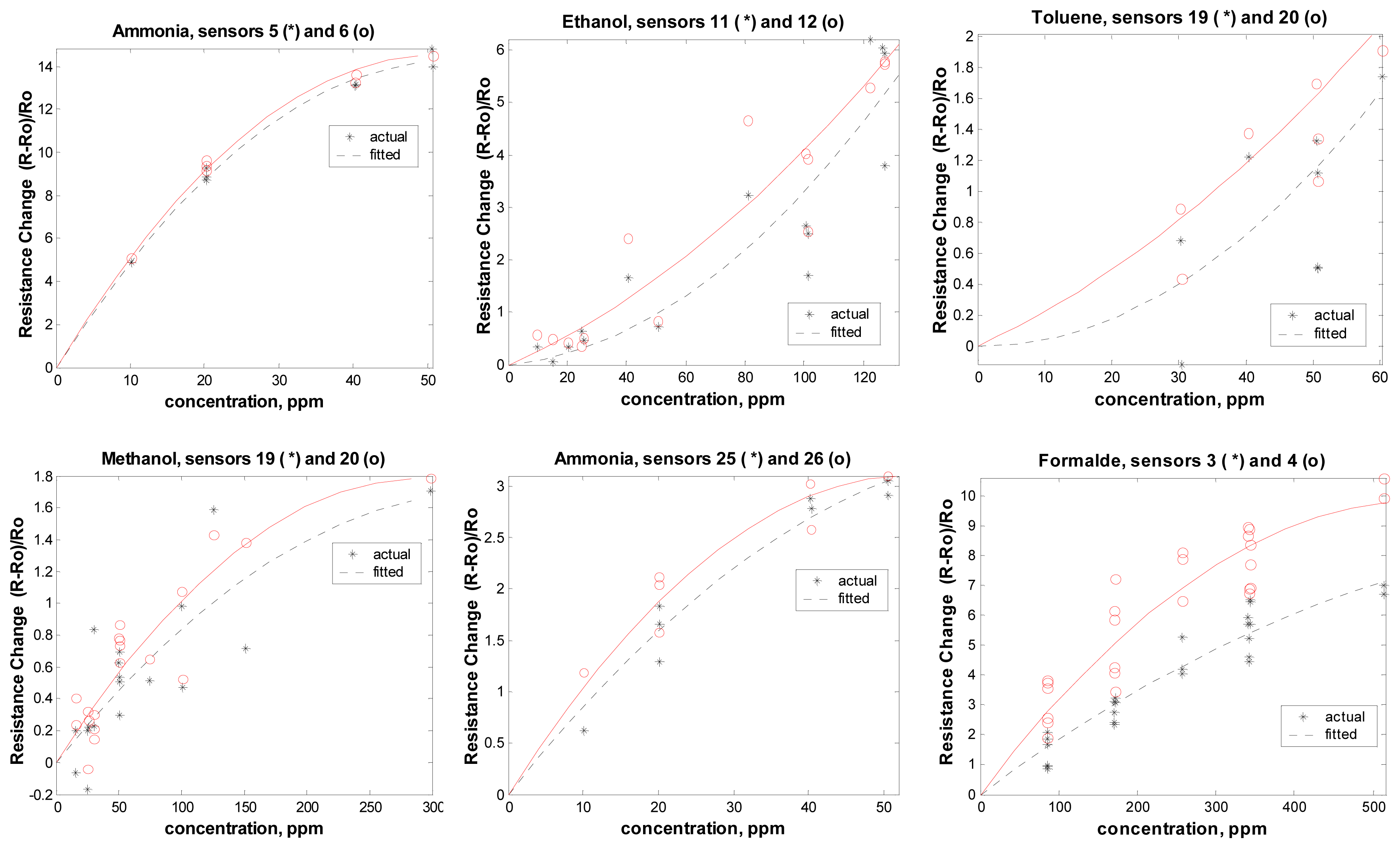
On obtaining a larger data set, it was observed that responses for some sensors were not linear for the concentration ranges considered; early tests that showed linear responses were done at substantially higher concentrations than the SMACs. Though the non-linearity appears to be of low order and applies to a few single analytes (see
Figure 2), they must be treated properly in order to reach the identification and quantification goals. Linearization of the response patterns with the LA based approach resulted in no significant improvement. At this point, we decided to develop a Levenberg-Marquardt nonlinear least squares method (LM-NLS) [
3], a natural step following the LA method.
NLS has been studied previously for analysis ion concentrations with an electrode sensor array [
14]. Kermani
et al. [
22] found that NN with a Levenberg-Marquardt learning algorithm showed satisfactory solutions for odor recognition. A comparison between nonlinear regression and NN models for pollution prevention focused on ground level ozone forecasting was reported by Cobourn
et al. [
23]. They found that non-linear regression models performed marginally better than the NN models in the hindcast mode (using observed meteorological data as input). Similar investigations reported by Shaffer
et al. compared the performance of neural network and statistical based pattern recognition algorithms. In general, NN, and particularly NNBP, based techniques were found to be slow and difficult to train, especially for noisy or high-dimension sensor data [
24].
The LM-NLS method demonstrated rapid operation speed and low memory requirements in addition to relative ease of training. Currently it takes 1-5 minutes to analyze each event on a non-dedicated Pentium III PC with MATLAB 5.3. That is quick enough to be used for “quasi real time” air monitoring. The computation time can be further reduced when optimized for real time code. The convergence problem can be improved by using multiple starting points as well as a modified update strategy (see Section 3, below) and is also relaxed by the fact that the quantification accuracy requirement in our case is rather tolerant.
3. Description of modified NLS algorithm
LM-NLS is similar to LA in that it tries to find the best-fit parameter vector x (concentrations) from an observation vector y (a response), which is related to x through a known linear or nonlinear function, y=f(A,x), where A describes system characteristics. A second order polynomial fit passing through the origin, y=A1x+ A2x2, is used to model the low-order nonlinearities found in our case. A1 and A2 are 1×32 matrices characterizing the 32 sensors' response to the twelve targeted compounds (ten analytes plus humidity change and a medical wipe, discussed below), which can be obtained from calibration data. Although, strictly speaking, the quadratic equation above can be solved analytically, we chose to use iterative optimization procedures to find the solution. This approach enables us to find a better (or best) solution instead of an exact one which might not make sense, and also allows for addition of potential better or other nonlinear models that we might be able to establish during the course of this project.
Our modified LM-NLS algorithm, which is based on an existing third party MATLAB code [
25], has the following implementation steps:
Begin with a starting point of xo; compute weighted residual vector: R=wt*(y-f(A,xo))
Compute Jacobian matrix J=dR/dx, curvature matrix C =JTJ, Jn=JC-1/2 and its diagonal D by SVD: Jn=UDVT, and gradient vector g=JnTR.
Update x with change Δx=V(D2+ε)-1/2g)C-1/2 and compute new residual vector R.
Repeat for various values of
ε as follows and update
x with a smaller sum-of-square (SOS) of residual
R and go to step 2 or stop at convergence:
- (a)
Set a series value of ε̣= [10-2, 10-1, 1, 102, 104].
- (b)
On the first iteration, search through the series of ε̣ to find x that results in the smallest residual. For subsequent iterations, multiply ε̣ by the (previously found; best ε value that produces minimum SOS in the last iteration and search through them.
Repeat Steps 1 through 4 for various starting points of vector xo: (starting points for this work are defined below)
- (a)
xo = [series-of-singles series-of-binary-mixtures…series-of-mixtures-of-all], and update x using the following scheme favoring a smaller number of significant elements (sig#):
- (b)
if (smaller-SOS & same-or-less-sig#) or (within-5% larger-sos & less-sig#) or (much(5%)-smaller-sos & sig# <4)
Through the course of the sensor development and training program, several modifications have been made to the original code (steps 1 through 4) to optimize ENose data analysis.
Sets of starting points of vector x were used instead of a single starting point of vector x. The purpose of using sets of starting points is to avoid converging to a local residual minimum, which is common in many iterative optimization algorithms and has been found for about ∼15-20% cases in our analysis with the original code. Ideally these initial sets of vector xo should be chosen randomly and cover each element's parameter space (detection range) uniformly. Alternatively, one can also choose the most likely combination of vector xo (of one element, of two elements,…, and of all elements). The total number of initial sets is determined by the speed desired and the complexity of the local minimum problem. In our case, about 200 initial sets (∼15*N, where N=12 is the number of target compounds) were found to be a compromise between good convergence properties and reasonable computing time. They include single gases at 5 different concentrations from low to high in the concentration range for each analyte (total ×12=60), two different combinations of binary mixtures of concentration low-high and high-low (total 12×11=132), and mixtures of all 12 analytes at 5 different concentrations from low to high (total 5). Combinations of ternary mixtures were not included in the current implementation but will be included in future versions of the algorithm.
We modify the updating strategy (implemented in Step 5 only) to favor a result with the sparest possible significant elements within certain ambiguity ranges of the residual, instead of always updating x for a smaller residual. Here significant elements refer to those elements whose values are equal to or greater than 1 ppm, except for indole, which is set at 0.001ppm.
Signature patterns for a given gas compound generated by the ENose sensor array have been observed to have large variations (see Fig.1). The standard updating strategy tends to minimize the residual with linear combinations of a number of gases when the residual is simply the variation in recorded response pattern itself and should be ignored. The modified strategy favors a smaller number of gas combinations within a certain ambiguity range of the residual, 5% in difference between the new and the best-so-far residuals. In doing so it also helps to minimize the possible linear dependency problem (see below), since most “high correlation” cases are found to be a linear combination of a large number of gases (4 or up), which is an “exact” solution does not make sense.
In addition to the above modifications to the algorithm, we also weighted the sensor response pattern to maximize the difference between similar signatures. Though the best efforts were made in selecting the set of polymers for the targeted compounds, final selection of the sensor set had to be made before full training sets were available to select an optimum set. As a result, in some cases, similar or linearly dependent signature patterns were observed for different target compounds,
e.g. ethanol and methanol, benzene and toluene, as shown in
Figure 1. The signature of benzene was also found in a previous experimental study to be a linear combination of the signature of toluene plus the signatures of other analytes in small concentrations [
19]. Regression analysis also confirmed the linear dependency among these signature patterns (
i.e. the signature for one analyte can be expressed as a linear combination of signatures from other analytes). Most other high correlation cases (correlation confidence > 0.85) are found to be a linear combination of four or more analytes. To reduce this similarity and linear dependency, the sensor raw resistance responses were modified by a set of weights in the data analysis procedure.
4. Experimental
The data analysis algorithm described above was developed to work with the JPL ENose sensor array, which was designed to be capable of monitoring the shuttle cabin environment for the presence of ten analytes at or below the 1-hour SMAC levels. Two additional analytes, water and a marker compound, were added to the list of target analytes over the course of the program. Target analytes were selected by reviewing results of analyses of the constituents of air collected in the space shuttle after several flights [
5] and selecting those that had been found with relatively high concentrations, although the concentrations of no analytes approached their SMACs. Additional compounds, such as ammonia, were selected because there had been anecdotal reports from shuttle crew members that an odor had been present at some time during a flight. As shown in
Table 1 [
1-
3], a total of ten potential contaminants were selected as target compounds. The ENose was also designed to be capable of detecting changes in humidity. After the flight experiment was defined, one target analyte was added to the list; a medical wipe saturated with 70% 2-propanol was used to provide a daily event or marker to verify device operation during the flight. The exact composition of the wipe is not known.
The sensors in the ENose are thin films made from commercially available insulating polymers loaded with carbon black as a conductive medium, to make a polymer-carbon composite. A baseline resistance of each film is established; as the constituents in the air change, the films swell or contract in response to the new composition of the air, and the resistance changes. Sensing films were deposited on ceramic substrates which had eight Au-Pd electrode sets. Four 25×10 mm
2 sensor substrates were used, with each sensing film covering a 2×1 mm
2 electrode set. 16 different polymers were used to make sensing film; each polymer was used to make 2 sensors for a total of 32 sensors. The polymers were selected by statistical analysis of responses of these films to a subset of the target compounds used [
1-
3].
Because the resistance in most of the polymer-carbon composite films is sensitive to changes in temperature, heaters were included on the back of the ceramic substrates to provide a constant temperature at the sensors. This constant temperature, 28, 32 or 36 °C, depending on ambient temperature, assisted vapor desorption and is sufficient to prevent hydrogen bonding of compounds sorbed in the polymer film.
For developing training sets and for testing, we used a gas delivery system built in our laboratory to deliver clean, humidified air with or without SMAC level analytes to the sensors. A detailed description of the gas delivery system can be found elsewhere [
26]. The gas handling system is run on house air that is cleaned and dehumidified with filters. The flow of air is controlled by a series of mass flow controllers, valves, and check valves. The air delivered to the sensors can be humidified by bubbling a fraction of the air through water and then remixing with dry air. To add a measured concentration of analyte (liquid or solid at room temperature) to clean air, a fraction of dry air is passed through liquid analyte, or over the solid, then mixed with the humidified air stream. Analyte concentrations are calculated from the saturated vapor pressure of the analyte, the temperature of the air above the analyte, and the total pressure in the bubbler. For analytes which are gaseous at room temperature,
e.g. methane, pure gas from a cylinder is connected directly to a mass flow controller and then mixed with clean humidified air. Calibrations of the system are done using a total carbon analyzer (Rosemont Analytical 400A) and checked in the JPL Analytical Chemistry Laboratory using Gas Chromatography-Mass Spectrometry (GC-MS). The gas delivery system is computer controlled using a LabVIEW program.
For normal operation, air is pulled from the surroundings into the sensor chamber at 0.25 L/min using a Thomas model X-400 miniature diaphragm pump. The air is directed either through an activated charcoal filter which is put in line to provide clean air baseline data, or though a dummy Teflon bead filter which is put in line to provide a pressure drop similar to that in the charcoal filter. A solenoid valve is programmed to open the path to the charcoal filter and provide clean air flow for a programmable period at programmable intervals; otherwise, the air is directed through the Teflon bead filter. Air then enters the glass enclosed sensor head chamber where resistance is measured. Typically, the charcoal filter was used for 15 minutes every 3.5 hours.
Data acquisition and device control are accomplished using a PIC 16C74A microcontroller and a Hewlett Packard HP 200 LX palm top computer which is programmed to operate the device, control the heaters and record sensor resistance. Typical normalized resistance change (dR/R0) for 10-50 ppm of contaminant is on the order of 2×10⁻⁴ (200 ppm resistance change), and may be as small as 1×10⁻⁵.
A preprocessing program extracts the resistance response pattern from raw resistance data for each detected event. Events were selected from the data using a peak searching program. Digital filtering was used for noise removal (high frequency) and baseline drift accommodation (slowly-varying in nature) before calculating the resistance change for each sensor in the array. Both relative resistance change, R/Ro, and fractional resistance change, (R-Ro)/Ro were tested, and the latter was adopted as it maximizes the difference between the signatures of different gas compounds.
5. Results and Discussion
5.1 Response analysis for single component
Before the ENose sensor was tested in flight (on-orbit), it underwent ground testing and training (lab-controlled gas events in clean air) comprised of over 250 events. These events include primarily single gas deliveries as well as some binary mixtures. For single gas events, the overall success rate is of the analysis algorithm is ∼ 85%, where success is defined as correctly identifying target compounds and quantifying them to +/− 50% of the known concentration. The success rates of identifying and quantifying single gases are listed in Table I, along with the concentration range tested (1-hr SMACs;. As can be seen from Table I, in some cases, i.e. ammonia, ethanol, indole, and propanol, it is possible to identify and quantify substantially below 30% of the one-hour SMAC; however, in a few cases quantification was successful only as low as 100% of the one-hour SMAC. In one case, formaldehyde, it was not possible to identify and quantify reliably below some two orders of magnitude above the one-hour SMAC.
For most gases, the success rate is higher for the higher end concentration range than for the lower end. For example, the success rate for methanol is 85% if the concentration range is 30ppm and above, for benzene it is 100% for the concentration range 20ppm and above, and for Freon it is 95% for the concentration range 65 ppm and above; the overall success rate is decreased by poor success at the lower end of the tested concentration range. This suggests that as long as the concentration exceeds the corresponding threshold, the algorithm can reliably identify and quantify a gas event. Among the 15% of cases that were classified as failed, about two-thirds (10% overall) are simply no detection of an event at low concentration, where poor repeatability is more evident. At these low concentration levels, although there are still measurable resistance changes in some of the sensors, the overall response patterns are so variable that the residual for a no-gas case would often be smaller than that for even the smallest concentration of any gas or gases. In other words, the response may be measurable but not large enough to be identified by either visual inspection or by the algorithm. For the remaining failures, the majority is due to incorrect identification (such as identification of toluene as benzene, owing to similarities in their fingerprints, see
Figure 1) instead of incorrect quantification. This indicates that the two-in-one (identification and quantification at once) NLS approach is largely adequate for quantification purpose; separation into two steps will improve little in terms of quantification accuracy, though it may help to improve identification in cases involving similar fingerprints.
5.3 STS-95 Flight Data Analysis
The ENose flight experiment was designed to provide continuous air monitoring during the STS 95 space shuttle flight (Oct.29 through Nov.7, 1998). The ENose was tested on STS-95 to confirm that sensor response and device operation are microgravity insensitive, and that the ENose would would be able to discriminate between responses caused by target analytes and odors associated with normal operation in the crew cabin. Although the ultimate goal of the program calls for real-time data analysis, it was determined for the current phase of the program that post-flight analysis would be preferable to running the risk of false positive data analysis in real time. The ENose sensor array response was recorded continuously for six days during the flight and data analysis was done post-flight. For the purpose of verification of the device operation over the six day experimental period a daily propanol-and-water medical wipe event was added as a daily marker. In addition, a daily air sample was collected using a Grab Sample Container (GSC) for later, independent GC-MS analysis at the NASA-JSC facilities.
The test the data analysis software faced was to detect gas events that were registered by the ENose sensor array, to identify and to quantify to +/−50% any targeted compounds in each gas event, and to classify non-targeted compounds as “unknown”. The events recorded were compared with shuttle logged events, planned experimental events, shuttle humidity and pressure logs and with independent, post-flight, GC-MS analysis of the air samples taken during the experiment.
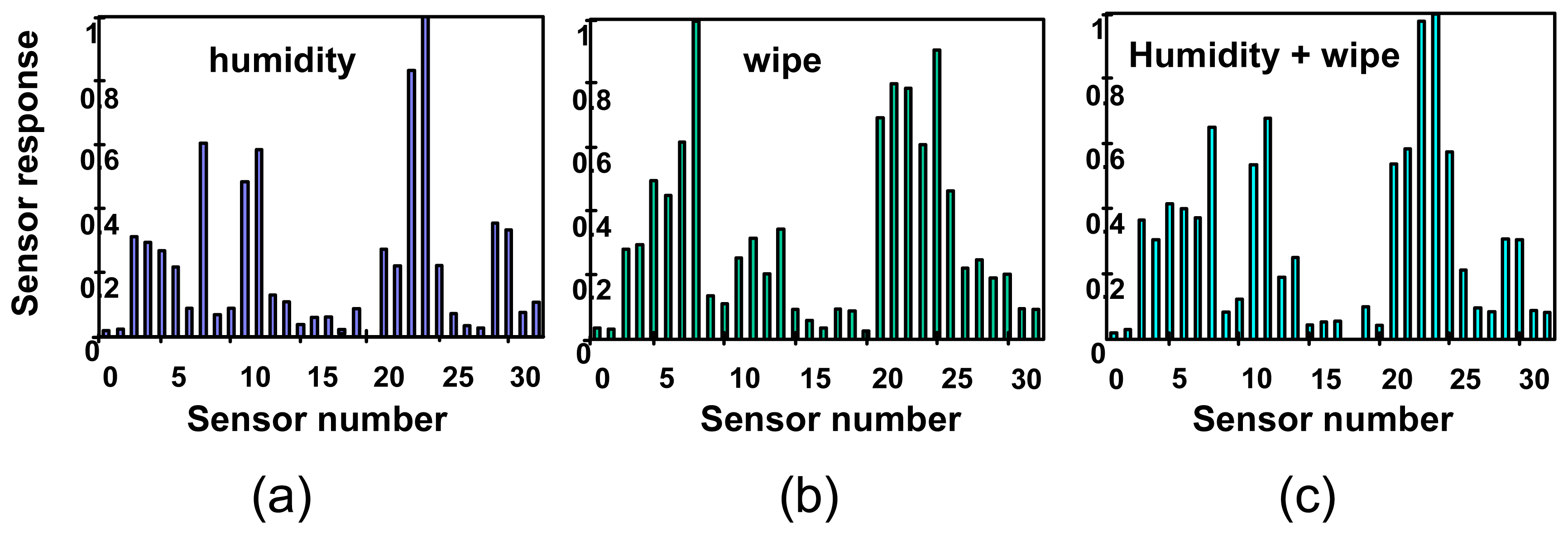
The automated peak searching feature of the data analysis software found 45 gas events in the data recorded by the ENose during the 6-day experiment. The 45 events were confirmed by visual inspection of the data; no other events were found by visual inspection. Among those recorded events, 6 were identified by the data analysis software as the planned daily markers, plus humidity changes in some cases. The concentrations of these marker events were quantified in the 500-1000 ppm range, which is the range found for similar tests done in the laboratory. These identifications were confirmed by comparison of crew log times with the time of the event in the data files. In addition to the marker events, software analysis identified all other events as humidity changes. Most of those changes can be correlated with cabin humidity changes recorded by the independent humidity measurements provided to JPL by NASA-JSC [
3]. Quantification by the ENose software corresponds to the relative humidity recorded by the cabin monitor. A few events were identified as humidity changes but did not correlate with cabin humidity logs. These events are likely to be caused by local humidity changes; that is, changes in humidity near the ENose device which were not sufficient to cause a measurable change in cabin humidity. The independent humidity monitor was located in the stairway between the middeck and the flight deck, and so would not record any humidity changes localized around the ENose. Software analysis of the flight data did not identify any other target compounds, as single gases or mixtures. Independent GC-MS analysis of the collected daily air samples confirmed that no target compounds were found in those samples in concentrations above the ENose training threshold. Also, there were no compounds that the ENose would have indicated as unidentified events present in the air samples. Fingerprints generated from flight data and corresponding to of each type of event found in the flight data, humidity change, daily marker, and daily marker plus humidity change, are shown in
Figure 4.
While it turned out to be an uneventful flight experiment and so did not challenge the data analysis routines significantly, the flight did serve the purpose of blind testing the software's ability to identify and quantify all registered events correctly, including planned events (daily markers, as single gases or as or mixtures) and unplanned events (humidity, as a single gas) which can be correlated to independent measures of cabin events, with no false positives. No inconsistencies were found between the data analysis results and the logged events, nor were there inconsistencies between the ENose data analysis and the independent GC-MS analysis. The ability of the data analysis algorithm to identify and quantify the dairly marker events confirms that the sensor response and operation of the ENose is microgravity insensitive.
6. Conclusion
A modified nonlinear least-squares based algorithm was developed as part of the JPL ENose program to identify and quantify single gases and mixtures of common air contaminants. The development of the NLS based method followed our early success with a linear algebra based method and later understanding of its limitation in nonlinear cases. It enables us to find a better (or best) solution instead of an exact one from noisy sensor response patterns. For lab-controlled testing, the algorithm achieved a success rate of about 85% for single gases in air and a moderate 60% success rate for mixtures of two compounds. The data set is characterized by large variations in response patterns, nonlinear responses in the concentration ranges considered, and similar fingerprints for a few compounds. The algorithm can reliably identify and quantify a gas event as long as the concentration exceeds the ENose sensor array detection threshold. During a six day flight experiment, the algorithm was able to identify and quantify all the changes in humidity and the presence of the daily marker detected and registered by the ENose sensor array. The lack of events in the flight experiment was evidence of the cleanliness of shuttle air, but disappointing for this test. Future testing will be focused on extensive ground testing, including blind testing of the software analysis in a relevant environment.
Future development of the JPL ENose requires the analysis software to include more capabilities, including real or quasi- real time analysis, and functional group classification of unknown gas compounds. Future work will also include improvements in the core LM-NLS algorithm itself. For example, the current algorithm uses all 32 sensors' responses as input. Though each sensor's response was weighted in the analysis in order to maximize the differences between similar signature patterns observed for different gas compounds, weights were determined empirically for this sensor set and were therefore not necessarily optimal. In the future, the selection of the sensor set to be used and their corresponding weights will be optimized by maximizing distances between gas signatures, defined as
, where dRm(i) is the ith sensor's normalized resistance change for the mth gas and the summation is over N sensors used.
Improvement of the NLS algorithm analysis speed is also desirable, not only for the purpose of real-time analysis, but also to accommodate the expanded target compound list and polymer set expected for the future generation of the ENose. Since the NLS algorithm is heavy with matrix operations, which largely determines the entire data analysis speed, increased size of the system characteristic matrix will slow analysis speed exponentially. One way to increase speed is to reduce the size of the matrix dynamically by incorporating sensors' characteristic response information, such as known negative or no responses of particular sensor(s) to certain gas compound(s). Besides increasing the speed, such information might also be used for compounds that are not trained for and therefore cannot be identified by the software, but might be classified by their functional group.


