A GNSS/INS/LiDAR Integration Scheme for UAV-Based Navigation in GNSS-Challenging Environments


1
Department of Civil Engineering, Toronto Metropolitan University, Toronto, ON M5B 2K3, Canada
2
Department of Civil Engineering, Faculty of Engineering, Zagazig University, Zagazig 44519, Egypt
3
Department of Civil Engineering, Tanta University, Tanta 31527, Egypt
*
Author to whom correspondence should be addressed.
Sensors 2022, 22(24), 9908; https://doi.org/10.3390/s22249908
Submission received: 11 November 2022
/
Revised: 7 December 2022
/
Accepted: 14 December 2022
/
Published: 16 December 2022
(This article belongs to the Section Navigation and Positioning)
Abstract
:Unmanned aerial vehicle (UAV) navigation has recently been the focus of many studies. The most challenging aspect of UAV navigation is maintaining accurate and reliable pose estimation. In outdoor environments, global navigation satellite systems (GNSS) are typically used for UAV localization. However, relying solely on GNSS might pose safety risks in the event of receiver malfunction or antenna installation error. In this research, an unmanned aerial system (UAS) employing the Applanix APX15 GNSS/IMU board, a Velodyne Puck LiDAR sensor, and a Sony a7R II high-resolution camera was used to collect data for the purpose of developing a multi-sensor integration system. Unfortunately, due to a malfunctioning GNSS antenna, there were numerous prolonged GNSS signal outages. As a result, the GNSS/INS processing failed after obtaining an error that exceeded 25 km. To resolve this issue and to recover the precise trajectory of the UAV, a GNSS/INS/LiDAR integrated navigation system was developed. The LiDAR data were first processed using the optimized LOAM SLAM algorithm, which yielded the position and orientation estimates. Pix4D Mapper software was then used to process the camera images in the presence of ground control points (GCPs), which resulted in the precise camera positions and orientations that served as ground truth. All sensor data were timestamped by GPS, and all datasets were sampled at 10 Hz to match those of the LiDAR scans. Two case studies were considered, namely complete GNSS outage and assistance from GNSS PPP solution. In comparison to the complete GNSS outage, the results for the second case study were significantly improved. The improvement is described in terms of RMSE reductions of approximately 51% and 78% for the horizontal and vertical directions, respectively. Additionally, the RMSE of the roll and yaw angles was reduced by 13% and 30%, respectively. However, the RMSE of the pitch angle was increased by about 13%.
1. Introduction
In unmanned air vehicle (UAV) navigation, the main challenge is to maintain accurate and robust estimation of the UAV position and orientation. Typically, global navigation satellite systems (GNSS) are used for UAV localization in outdoor environments. However, GNSS signals may suffer from degradation or outages due to a signal blockage or a malfunction, which leads to a vulnerable system if it relies exclusively on GNSS. Therefore, the navigation system must possess redundancy to ensure reliability and availability. This emphasizes the need for multi-sensor integration to achieve reliable autonomous navigation [1,2,3]. In addition, recent developments in sensor technology have increased the payload capabilities of UAVs to include multiple sensors, such as cameras and light detection and ranging (LiDAR).
An inertial navigation system (INS) uses an inertial measurement unit (IMU) to measure the rotation rate and acceleration, which are used to obtain the UAV pose (i.e., position and the attitude) [4,5,6]. However, low-cost MEMS-based IMU measurements suffer from significant drift over time. Consequently, another sensor is required to constrain the drift, such as GNSS [7]. GNSS-aided INS is the most common navigation system [8,9]. Typically, Kalman filter is used to fuse the observations of the GNSS and IMU [10]. For example, in loosely coupled (LC) integration, the INS mechanization provides the position of the vehicle at a high frequency. GNSS updates are fed into the system at a lower frequency to minimize the INS solution drift. Due to the closed-error scheme integration, the INS can provide long-term stability with high accuracy while experiencing occasional short-period GNSS signal outages [11]. However, if the GNSS signal outage persists for a long period, the system will be reliant on the performance of the INS, which has a diverging error nature, especially when a low-cost IMU is used [12,13,14,15,16].
An alternative approach is to use additional onboard sensors, such as cameras and LiDAR sensors, in order to sustain accurate pose estimation of the UAV during GNSS outages. Vision-based navigation systems are mainly integrating visual sensors with the inertial unit through simultaneous localization and mapping (SLAM) techniques, such as ORB-SLAM2 [17] and VINS-Mono [18]. The basic idea of SLAM algorithms is to keep track of the sensor location while simultaneously constructing a map of the surrounding environment [19]. Nevertheless, the camera sensors are susceptible to illumination changes and require detecting sufficient features in the surrounding environment. Consequently, these systems will not operate properly in light-changing situations or featureless areas.
On the other hand, LiDAR sensors are widely used for navigation using SLAM techniques. Many studies have investigated the use of LiDAR for UAV navigation [20,21,22]. In 2014, the LiDAR odometry and mapping (LOAM) algorithm was presented as one of the leading algorithms [23], which is ranked third on the KITTI benchmark [24]. Subsequently, other variants and modified versions of LOAM were presented, including, A-LOAM [25], LeGO-LOAM [26], optimized LOAM SLAM by kitware [27], R-LOAM [28], and F-LOAM [29]. Improving the processing time of the LOAM algorithm was the common theme among these SLAM algorithms. For UAV navigation, LiDAR is typically used for mapping applications. However, it can potentially be used for navigation to complement onboard positioning sensors.
GNSS/INS/LiDAR SLAM integration has been investigated by a number of researchers. In [30], a three-dimensional reduced-inertial-sensor system (3D-RISS) was integrated with LiDAR odometry and GNSS through an extended Kalman filter (EKF). The position and azimuth estimated using LiDAR odometry were used to update the 3D-RISS mechanization. The proposed approach was tested for various driving scenarios in Kingston and downtown Toronto, Canada. In comparison with the INS solution, the RMSE of the position in the horizontal direction was reduced by 64%. In [31], graph optimization LiDAR SLAM was integrated with GNSS/INS, where the GNSS/INS results were matched with the relative pose of a 3D probability map. The integrated scheme was tested during a one-minute outage of the GNSS signal, which resulted in reductions in RMSE by 80% approximately. In [32], a similar approach was proposed; however, an odometer was added to the integrated scheme. The system was tested during a 2-min GNSS outage. The integration results showed a reduction in the north, east, and height directions RMSE by 62.8%, 72.3%, and 52.1%, respectively, in comparison with the GNSS/INS integrated system counterpart. In [33], an INS/LiDAR SLAM terrestrial navigation system was developed. The data source in that study was the raw KITTI dataset for both residential and highway drives [24]. Three case studies with different driving scenarios were considered in order to test the robustness of the developed integrated navigation system. The proposed model outperformed a number of the literature LiDAR SLAM algorithms. A similar approach to the one adopted in [33] will be used in this current study, albeit for an UAV navigation.
In this study, an integrated UAV-based GNSS/INS/LiDAR SLAM navigation system is developed. The proposed approach is developed to overcome frequent and prolonged GNSS outages resulting from an unexpected antenna malfunction during data collection. The data has been collected using a DJI Matrice-600 UAV equipped with the Velodyne PUCK LiDAR sensor (previously VLP-16), a Sony α7R II camera, and the Applanix APX-15 UAV GNSS/INS. The system implements a loosely-coupled integration that takes advantage of the LiDAR SLAM solution (latitude, longitude, altitude, pitch, roll, and yaw) to update the INS solution in a closed-error loop scheme using an EKF. The remainder of this paper is organized as follows: Section 2 presents the UAV data collection platform, data acquisition, and data preprocessing. The system architecture and models are explained in Section 3. Section 4 discusses the experimental results, and finally conclusions are presented in Section 5.
2. Data Acquisition and Preprocessing
2.1. Data Acquisition
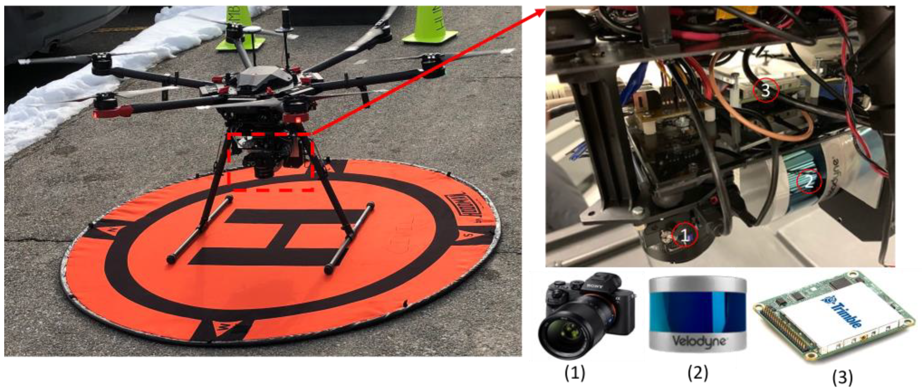
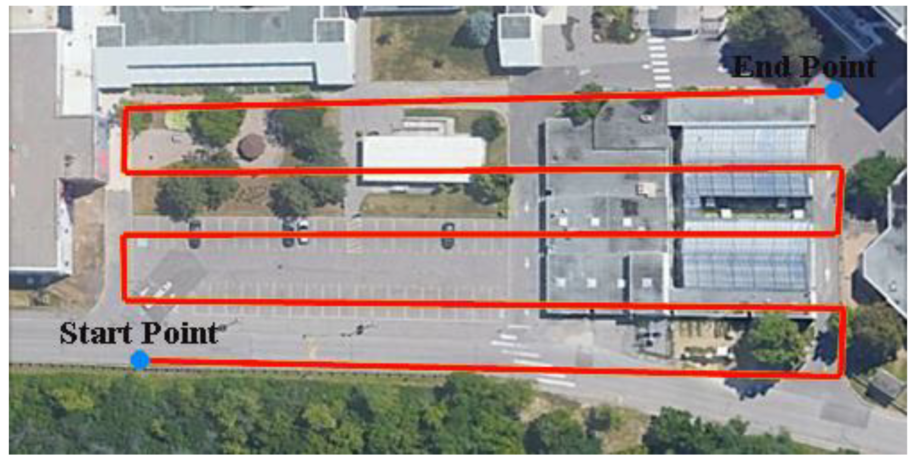
In this study, a UAV was used as the platform for data acquisition. The UAV consisted of a DJI Matrice 600 Pro carrying a Sony α7R II RGB camera, a Velodyne PUCK LiDAR sensor, and the Applanix APX-15 UAV GNSS/INS board. Figure 1 shows the system components and how the various sensors are rigidly fixed within the UAV platform. The Sony α7R II camera has a 42.4 MP spatial resolution with a 7952 × 5304 image size [34]. The images were acquired based on distance, rather than time interval, with an average frame rate of 0.5 Hz, and the number of captured images was 110 images. The Velodyne PUCK, on the other hand, consists of 16 laser beams with a 360° horizontal field of view (FOV) and a 30° vertical field of view. The PUCK maximum range measurement is 100 m with a 3 cm range accuracy [35]. The total number of acquired points was approximately 14 million points at a 10 Hz frame rate. The Applanix APX-15 UAV GNSS/INS unit was used in this study due to its low weight, compact size, and precise positioning and orientation information [36]. The GNSS data was collected at a 10 Hz, while the IMU data was collected at a 200 Hz frame rate. In order to cover the area of interest, the flight was performed at approximately 25 m above the ground, acquiring the data in 5 parallel flight lines. Figure 2 shows a top view of the flight trajectory over the area of interest.
2.2. Data Preprocessing
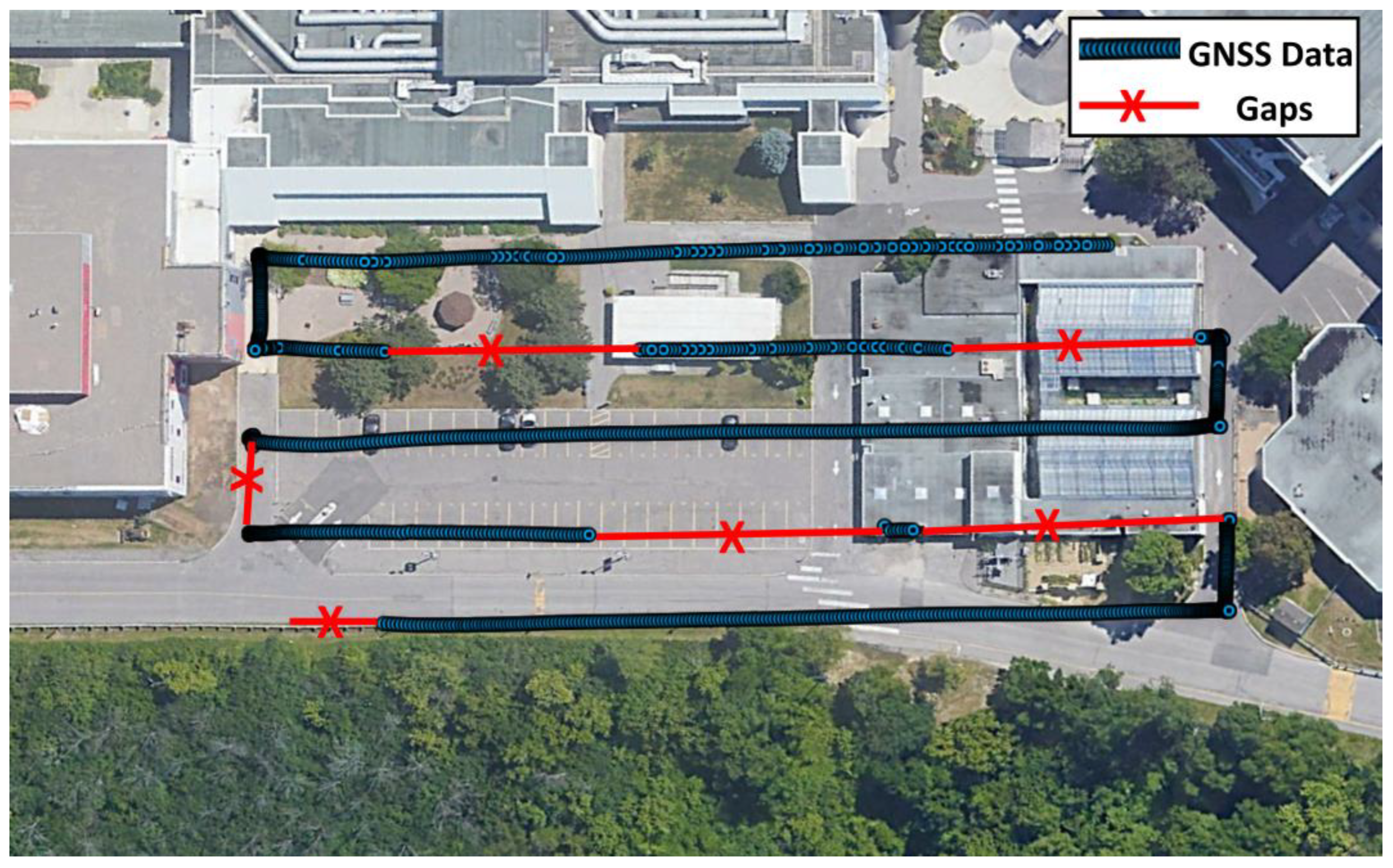
Applanix POSPac UAV software [37] was used to process the collected GNSS/IMU data in differential mode to obtain the precise drone trajectory. Unfortunately, the software crashed after obtaining an error that exceeded 25 km. Investigating the reason revealed the fact that there were numerous prolonged GNSS signal outages due to a malfunction, as shown in Figure 3. The software estimation filter could not handle the large drift of low-cost IMU. An attempt was made to process the GNSS-only data in differential mode, which also failed. The GNSS data was then processed in precise point positioning (PPP) mode using the Canadian Spatial Reference System PPP (CSRS-PPP) service by Natural Resources Canada (NRCan) [38], which was successful, but the obtained results were at dm-m level accuracy with many gaps. The PPP results indicated that the drone altitude was not uniform (with variation in the range of 5 m), which might have been caused by a mass imbalance in the UAS. Partial or complete reset of the ambiguity parameters were performed frequently, which indicates that the PPP results were essentially code-based, i.e., with degraded accuracy.
As a result of POSPac crash and the unavailability of precise GNSS/INS solution, the camera images had to be processed using ground control points (GCPs) to enable a precise UAV trajectory, which can then serve as ground truth. Twelve checkerboard targets were deployed at the study site, as shown in Figure 4, The precise coordinates (centimeter-level) of the targets were determined using a dual-frequency SOKKIA GCX2 GPS receiver in the real-time kinematic (RTK) mode. The RGB images were processed with the four corner GCPs (green boxes) using Pix4D mapper software [39] to estimate the camera poses. The other eight points (blue boxes) were used as check points. Figure 5 shows the estimated poses of the camera using the Pix4D mapper software. Table 1 shows the absolute camera position and orientation error statistics.
Finally, the LiDAR data were processed using the optimized LOAM SLAM algorithm based on LOAM [23,27]. optimized LOAM SLAM was adopted over GraphSLAM algorithms, as the latter are generally more computationally expensive, such that they consider all pose estimates in the calculation process. By contrast, EKF-based SLAM methods consider the last pose only [40].
The improved LOAM SLAM consists of three sequentially performed steps: key point extraction, LiDAR odometry, and LiDAR mapping. In the first stage, the critical points are categorized based on their curvature as either edges or planar points. Planar points correlate to the smallest curvature, whereas edge points correspond to the highest curvature. In the LiDAR odometry stage, a modified version of the iterative closest point matching algorithm is employed to reconstruct the LiDAR motion between two consecutive frames. Depending on the feature type, the distance between a point and a line or a point and a plane can be calculated. Finally, the recovered motion is refined by projecting the current frame onto the existing map and comparing it to it. More details about the LOAM SLAM can be found in [23].
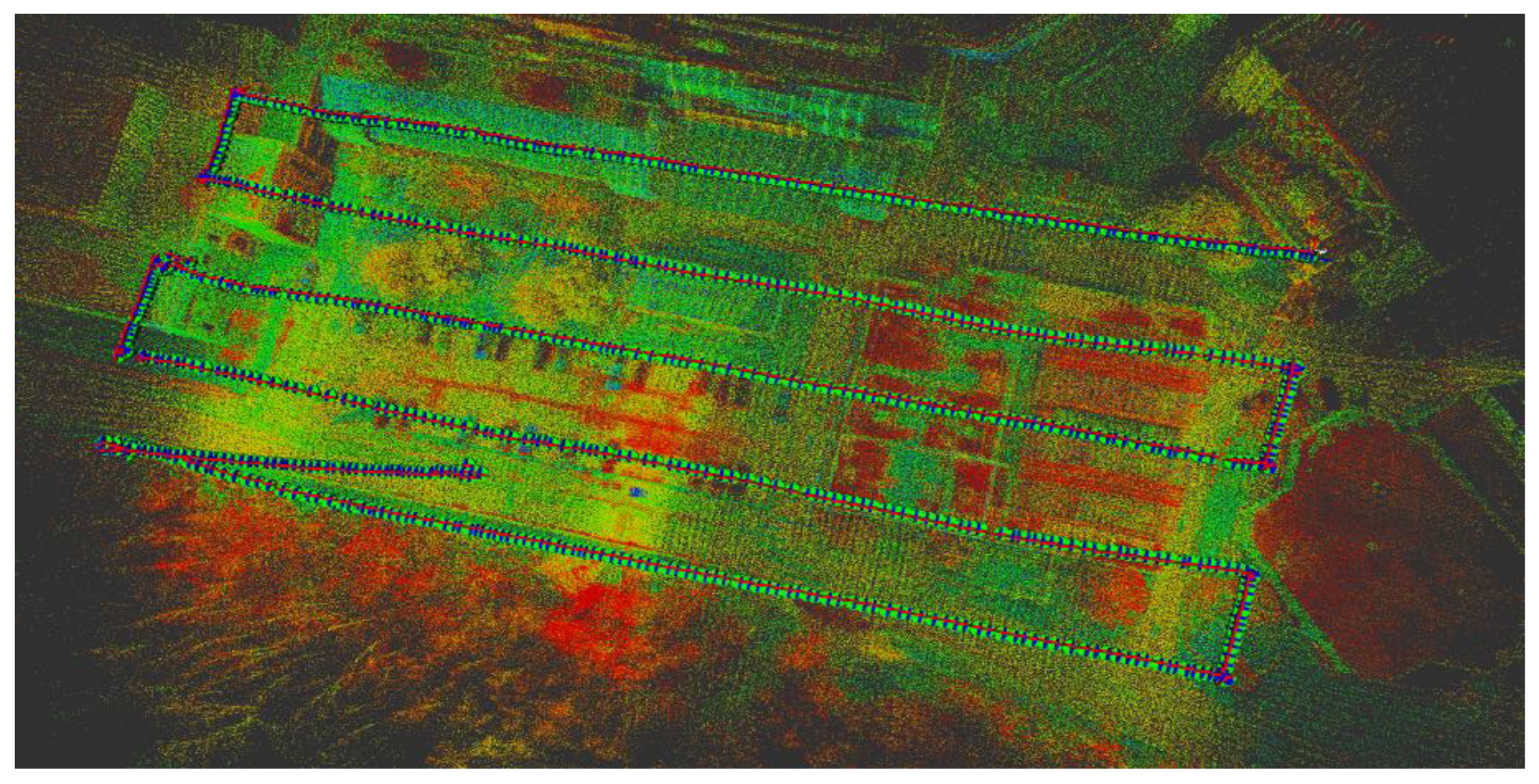
Optimized LOAM SLAM is an enhanced variant of LOAM. The execution time is shortened due to the utilization of C++ libraries and tools optimized for improved computational speed. In addition, the method is not dependent on hard-coded parameters and can be run on either robot operating system (ROS) or LiDARView software. In addition, it is more generalized so that it operates on multiple LiDAR sensors, including Velodyne sensors. However, it is essential to highlight that optimized LOAM SLAM neither currently conducts loop closure nor it incorporates IMU measurements in the scan matching of successive frames. In this research, the optimized LOAM SLAM algorithm was executed on ROS. Two Python nodes (pc saver and traj saver) were created to subscribe to the trajectory and point cloud topics and preserve their respective outputs. Figure 6 and Figure 7 [41] show the LiDAR SLAM trajectory and the generated point cloud, respectively.
2.3. Data Synchronization
All collected data were synchronized through GPS time stamp and resampled to 10 Hz to ensure correct data correspondence which is essential for subsequent processing stages. As such, the IMU data were downsampled from 200 Hz to 10 Hz for the raw accelerometers and gyroscopes measurements. Conversely, the camera pose estimations produced by Pix4D Mapper were up-sampled from approximately 0.5 Hz to 10 Hz. The resampling was accomplished using linear interpolation.
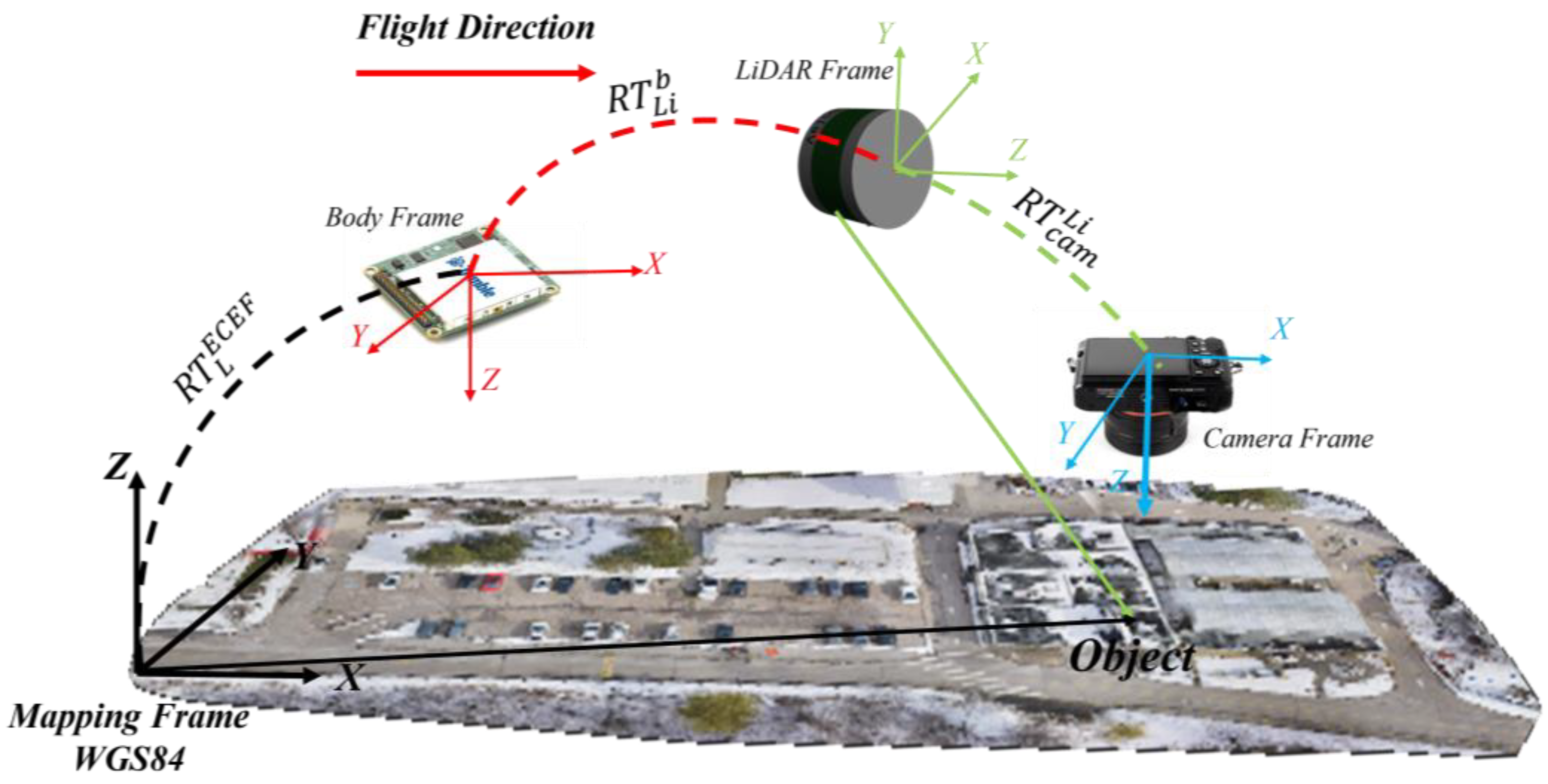
Subsequently, coordinates transformation was performed to have all pose estimation in the same reference frame. The position and rotation transformations were executed using a homogenous transformation using 4 × 4 transformation matrices, which is computationally efficient. The LiDAR pose estimates were transformed from the local frame of the first point cloud of the Velodyne sensor stream into the WGS84 reference frame. Figure 8 depicts a graphical illustration of the sequence of transformations.
Let denotes a point captured in the local frame of the LiDAR and let denotes the same point expressed in the WGS84 reference frame. The sequence of homogenous transformations is presented by Equations (1) and (2).
where is the homogenous transformation matrix from the l-frame to the WGS84 frame, is the homogenous transformation matrix from the b-frame to the l-frame, is the homogenous transformation matrix from the LiDAR frame to the b-frame, is the rotation matrix from the LiDAR frame to the l-frame, and is the rotation matrix from the LiDAR frame to the b-frame.
3. System Architecture and Mathematical Models
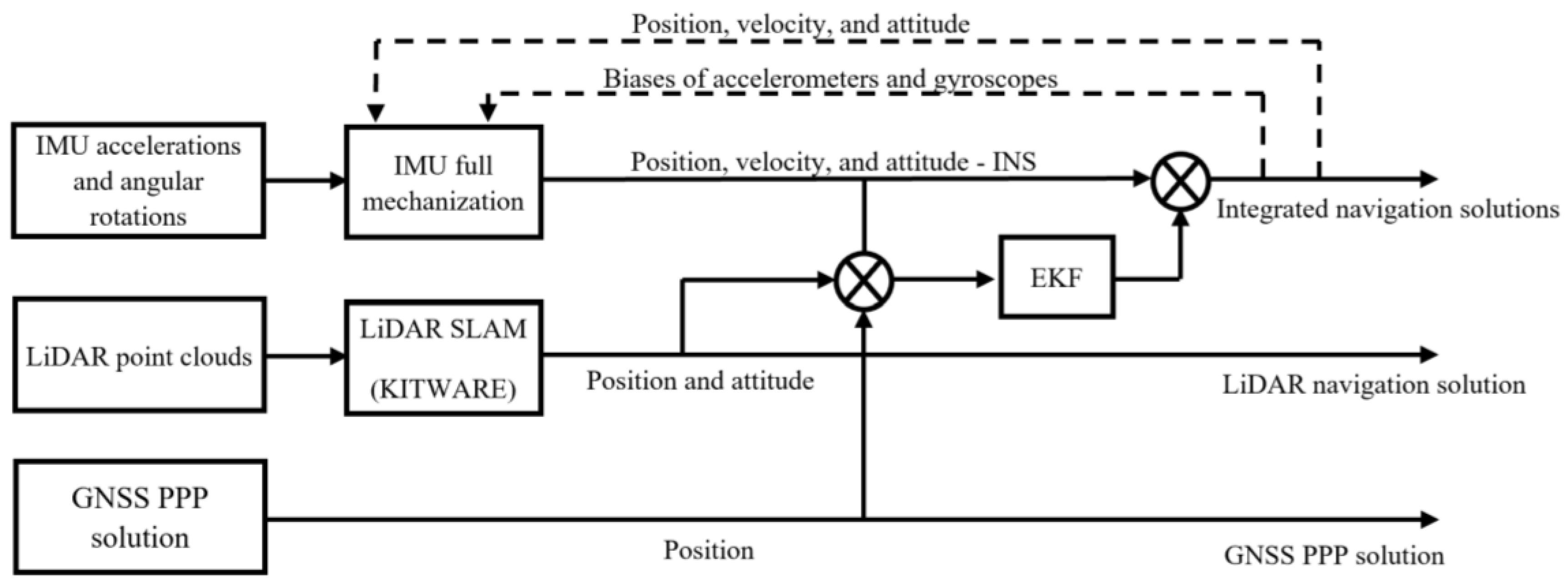
A loosely coupled integration between the INS and the LiDAR SLAM is implemented using an EKF, which results in an integrated navigation solution. As shown in Figure 9, the raw IMU measurements are fed into a full IMU mechanization, which produces the position, velocity, and attitude angles of the inertial navigation system. The LiDAR scans are used as input to the optimized LOAM SLAM algorithm, which results in the position and attitude of the UAV. These are used as the measurement update to the IMU mechanization output during the update stage of the EKF. The result is the integrated INS/LiDAR navigation solution. The updated errors are fed back into the IMU mechanization, which forms a closed-loop error scheme. Two case studies were considered. The first one is a complete absence of the GNSS signal throughout the full UAV trajectory. In this case, the measurement update is from the LiDAR SLAM only. The second case study, on the other hand, includes updates from the GNSS PPP solution every 20 s.
The EKF system model, measurement model, and other mathematical and stochastic equations are similar to [33]. In the prediction stage, the state vector is defined by Equation (3). Subsequently, in the update stage, the measurement update vector is given by Equation (4).
where is the position error vector; is the velocity error vector, is the attitude angles’ error vector; is the accelerometer bias error vector; is the gyroscope bias error vector; , , are the measurement errors for the geodetic latitude, longitude and height; and , , are the measurement errors for the pitch, roll, and yaw angles.
4. Results and Analysis
4.1. First Case Study—Complete GNSS Outage
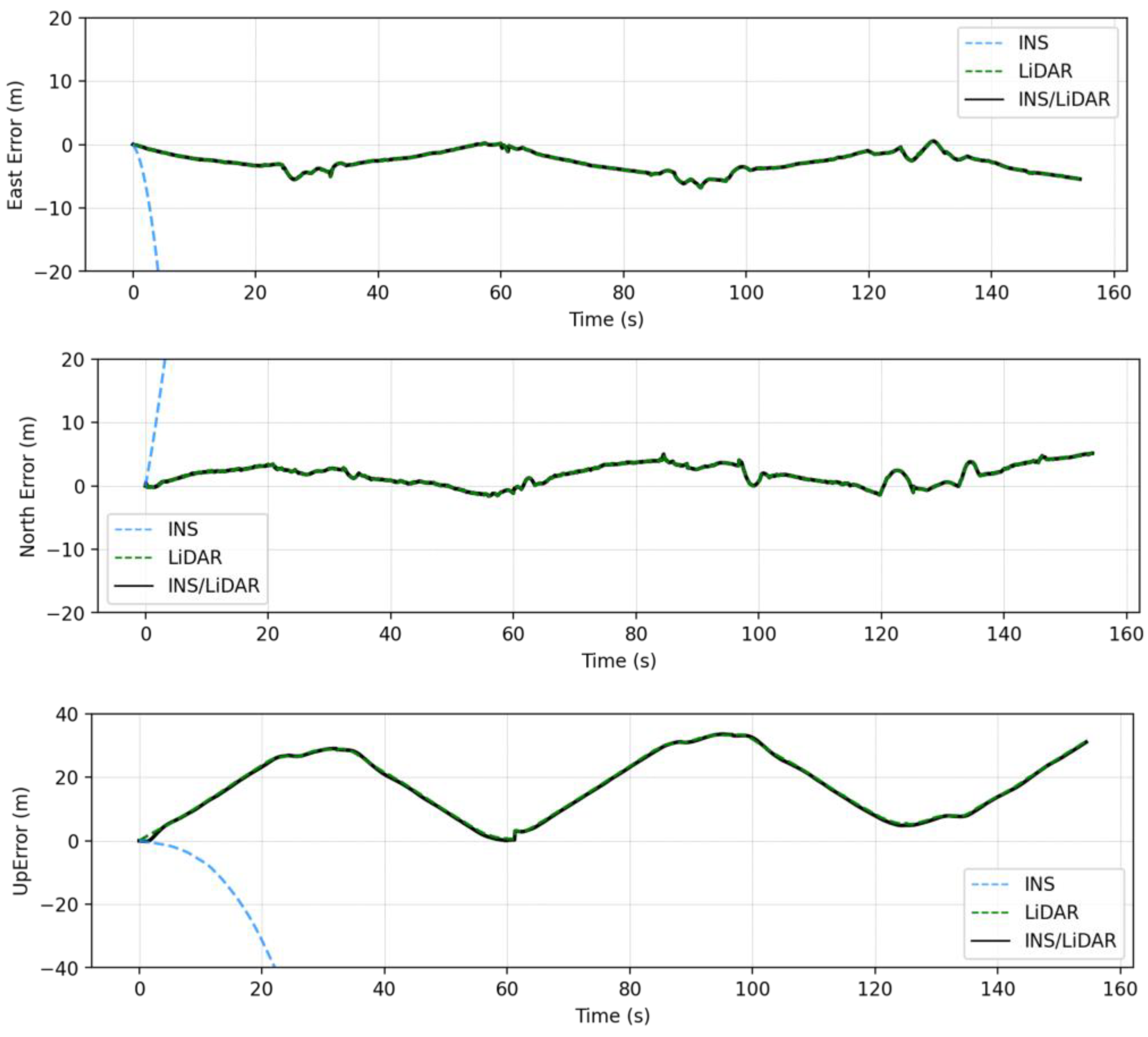
In this case study, a full GNSS signal outage is assumed along the whole trajectory of the UAV. Three navigation solutions were considered in this case study, namely, INS-only, LiDAR SLAM-only, and the integrated INS/LiDAR SLAM solution. The INS-only solution represents the solution obtained through IMU mechanization, while the LiDAR SLAM-only solution is the one produced using the optimized LOAM SLAM. Finally, the third solution is the integrated INS/LiDAR SLAM solution using EKF. The position and attitude of the three navigation solutions were compared to the ground truth, which is the interpolated camera solution. Figure 10 shows the position errors in the ENU local reference frame, while Figure 11 illustrates the errors of the attitude angles (roll, pitch, and yaw) for three navigation solutions. The error statistics of the position and attitude are shown in Table 2 for the three navigation solutions.
Figure 10 shows that the INS solution drifts significantly over time, indicating that it cannot be used solely for accurate navigation. However, in comparison with the INS solution, the integrated navigation system produced significantly less errors. Therefore, the integrated system was tuned to increase the weights of LiDAR SLAM position updates, while lowering those of the INS solution. As a result, the combined INS/LiDAR position solution was somewhat similar to the LiDAR SLAM solution. As shown in Figure 10 and Table 2, the up-direction error is significantly larger than the horizontal counterpart. The reason for this behavior is due to the nature of the collected point clouds, such that the distribution of the points is only in one direction (below the lidar sensor), which causes poor vertical geometry. Similar behavior was presented in [33], where the estimations for the up-direction from the LiDAR SLAM was sensitive to the geometry of the detected features.
In contrast, the integrated INS/LiDAR solution in Figure 11 was tuned to follow the INS solution for pitch and roll angles, which outperformed those of the LiDAR SLAM. However, the integrated system followed the yaw angle produced by the LiDAR SLAM, which was more accurate than that of the INS solution. It is worth mentioning that the IMU measures the vehicle’s accelerations and angular rotations directly, after which the attitude was estimated, which leads to more accurate estimations for the attitude in comparison to position estimation. However, when the drone performs sharp turns, the yaw angles estimations from the IMU mechanization drifts significantly, in which case, the LiDAR SLAM estimates are better for the yaw. This behavior echoes with [33] for the pitch and roll angles, albeit not the yaw angle. The reason for this is due the different nature of the datasets, terrestrial in [33] versus UAV system in this paper. The yaw angle estimate from the IMU mechanization in case of UAV navigation will be more sensitive to turns because the UAV turns are typically drastically sharper than those of cars.
The RMSE of the integrated INS/LiDAR position errors and the yaw angle converged towards that of the LiDAR SLAM, while the RMSE of the pitch and roll angles were closer to that of the mechanization errors. In Figure 12, LiDAR SLAM and INS/LiDAR trajectories are compared to the ground truth for the first case study (complete GNSS signal outage).
4.2. Second Case Study—GNSS PPP Assistance
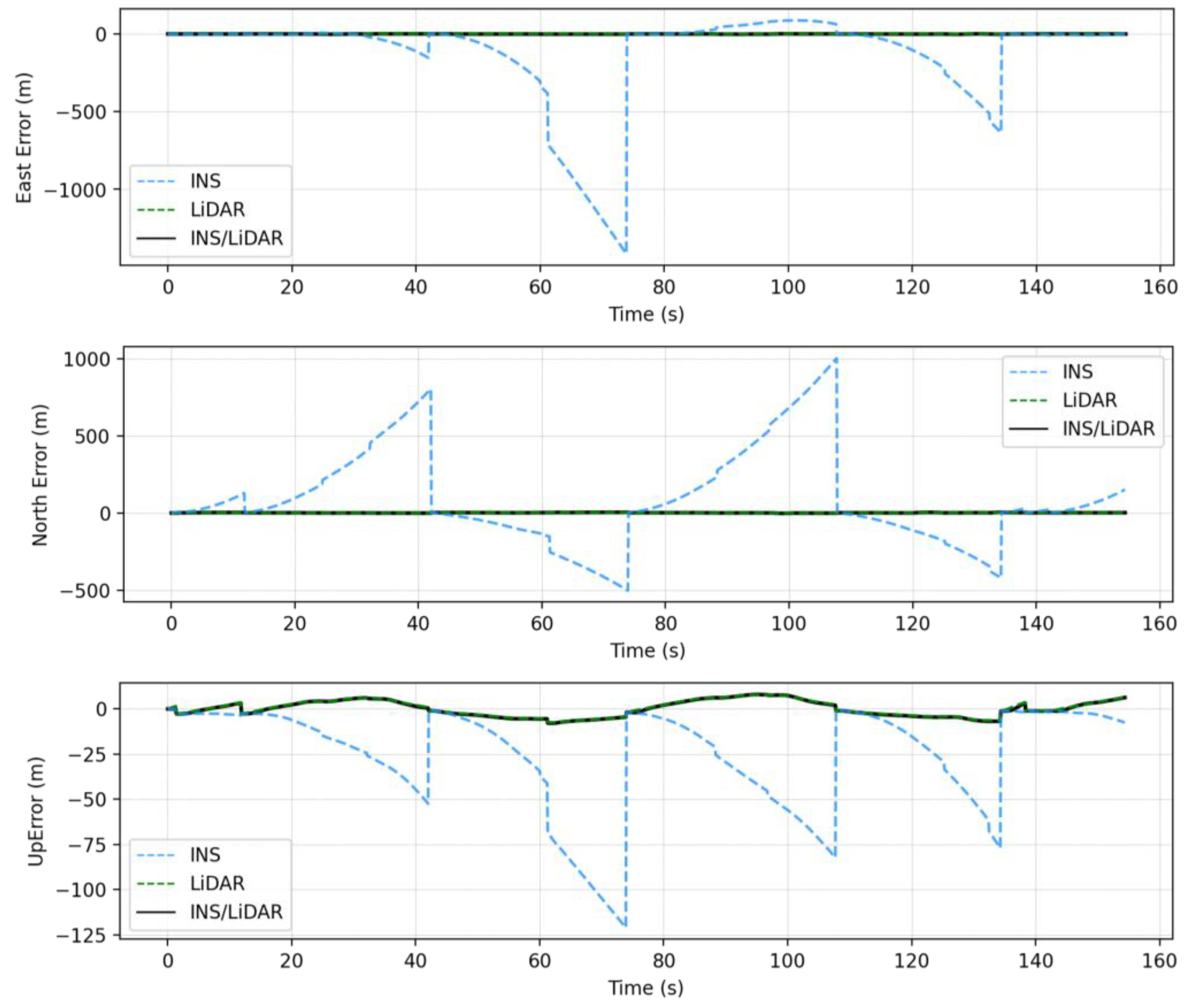
In the second case study, updates from the GNSS PPP solution were considered to improve the LiDAR SLAM results, and thereby fill in the GNSS gaps, as mentioned in Section 2. The GNSS position updates are fed into the EKF every 20 s, whenever they are available, while the filter continued to receive attitude updates from the LiDAR SLAM.
The same approach for the filter tuning was adopted as discussed in the first case study. As a result, a similar performance can be observed for the position and attitude errors of the integrated system (Figure 13 and Figure 14). However, as shown in Table 3, the errors are significantly reduced in comparison with the previous case study, which is attributed to the GNSS updates. A comparison between LiDAR SLAM and GNSS/INS/LiDAR trajectories with respect to the ground truth for the second case study is shown in Figure 15. As shown in Table 4, it is noticeable that the GNSS updates led to a lower RMSE of approximately 51% and 78% in the horizontal and up directions, respectively. Additionally, the reductions in the RMSE of the roll and yaw angles were roughly 13% and 28%, respectively. However, there existed no significant change in the pitch angle.
It is worth mentioning that the positioning accuracy for this case study mainly depends on that of the PPP solution. As mentioned in Section 2.2, the accuracy of the GNSS PPP solution was in the dm-m level accuracy. Should a higher precision PPP solution be available, the integrated solution will follow.
5. Conclusions
In this study, a GNSS/INS/LiDAR integrated navigation system was developed to overcome numerous and prolonged GNSS signal outages caused by a malfunctioning GNSS antenna during data collection. To recover the full trajectory of the UAV, the LiDAR data were processed using the optimized LOAM SLAM algorithm, which yielded position and rotation estimations of the sensor. The camera images were processed with the help of four corner GCPs using Pix4D Mapper software, which resulted in precise camera poses that served as ground truth. All collected sensor data were timestamped by the GPS time, and therefore all datasets were synchronized to match the same frequency of the LiDAR data. Two case studies were considered. In the first case study, a LC integration between the INS and the LiDAR SLAM solution was implemented using an EKF. The positioning accuracy of this case study depends mainly on the LiDAR SLAM accuracy, which yielded a larger error in the up direction in comparison with the horizontal direction. This is essentially caused by the poor vertical geometry. In contrast, the integrated INS/LiDAR solution was tuned to follow the INS solution for pitch and roll angles, which outperformed those of the LiDAR SLAM. However, the integrated system followed the yaw angle produced by the LiDAR SLAM, which was more accurate than that of the INS solution.
A similar integration was executed in the second case study, albeit with updates from the GNSS PPP solution every about 20 s. The same approach for filter tuning was adopted as in the first case study. It was shown that significant improvement in the latter case is obtained in the pose estimation compared to the full absence of GNSS. The positioning RMSE was reduced by 51% and 78% in the horizontal and up directions, respectively, while the RMSE of the roll and yaw angles was reduced by 13% and 28%, respectively. However, the RMSE of the pitch angle was increased by about 13%.
Author Contributions
Conceptualization and methodology: A.E.-R., A.E. and N.A.; software: A.E. and N.A.; validation: N.A. and A.E.; formal analysis: N.A. and A.E.; writing—original draft preparation, A.E. and N.A.; writing—review and editing: A.E.-R.; supervision, A.E.-R. All authors have read and agreed to the published version of the manuscript.
Funding
This research is supported by Natural Sciences and Engineering Research Council of Canada (NSERC) RGPIN-2022-03822, the Government of Ontario, and Toronto Metropolitan University.
Institutional Review Board Statement
Not applicable.
Informed Consent Statement
Not applicable.
Data Availability Statement
The data presented in this study are not publicly available.
Acknowledgments
The authors would like to thank Akram Afifi, a professor in the Faculty of Applied Sciences and Technology, Humber College, for providing the dataset used in this research. The authors would also like to thank Kitware for making its SLAM package available.
Conflicts of Interest
The authors declare no conflict of interest.
References
- Perez-Grau, F.J.; Ragel, R.; Caballero, F.; Viguria, A.; Ollero, A. An architecture for robust UAV navigation in GPS-denied areas. J. Field Robot. 2018, 35, 121–145. [Google Scholar] [CrossRef]
- Balamurugan, G.; Valarmathi, J.; Naidu, V. Survey on UAV navigation in GPS denied environments. In Proceedings of the 2016 International Conference on Signal Processing, Communication, Power and Embedded System (SCOPES), Paralakhemundi, India, 3–5 October 2016. [Google Scholar]
- Martínez-Díaz, M.; Soriguera, F. Autonomous vehicles: Theoretical and practical challenges. Transp. Res. Procedia 2018, 33, 275–282. [Google Scholar] [CrossRef]
- Samadzadegan, F.; Abdi, G. Autonomous navigation of Unmanned Aerial Vehicles based on multi-sensor data fusion. In Proceedings of the 20th Iranian Conference on Electrical Engineering (ICEE2012), Tehran, Iran, 15–17 May 2012; pp. 868–873. [Google Scholar]
- Kim, J.; Sukkarieh, S. Autonomous airborne navigation in unknown terrain environments. IEEE Trans. Aerosp. Electron. Syst. 2004, 40, 1031–1045. [Google Scholar] [CrossRef]
- Kim, J. Autonomous Navigation for Airborne Applications. Ph.D. Thesis, University of Sydney, Camperdown, Australia, 2004. [Google Scholar]
- Saeedi, S.; Samadzadegan, F.; El-Sheimy, N. Vision-aided inertial navigation for pose estimation of aerial vehicles. In Proceedings of the 22nd International Technical Meeting of The Satellite Division of the Institute of Navigation (ION GNSS 2009), Savannah, GA, USA, 22–25 September 2009; pp. 453–459. [Google Scholar]
- Kim, J.-H.; Sukkarieh, S. Flight test results of GPS/INS navigation loop for an autonomous unmanned aerial vehicle (UAV). In Proceedings of the 15th International Technical Meeting of the Satellite Division of The Institute of Navigation (ION GPS 2002), Portland, OR, USA, 24–27 September 2002; pp. 510–517. [Google Scholar]
- Wang, R.; Hou, X.; Liu, F.; Yu, Y. GPS/INS Integrated Navigation for Quadrotor UAV Considering Lever Arm. In Proceedings of the 2020 35th Youth Academic Annual Conference of Chinese Association of Automation (YAC), Zhanjiang, China, 16–18 October 2020; pp. 132–136. [Google Scholar]
- Shin, E.-H. Estimation Techniques for Low-Cost Inertial Navigation; UCGE Report, Number 20219; University of Calgary: Calgary, AB, Canada, 2005. [Google Scholar]
- Noureldin, A.; Karamat, T.B.; Georgy, J. Fundamentals of Inertial Navigation, Satellite-Based Positioning and Their Integration; Springer Science & Business Media: Berlin/Heidelberg, Germany, 2012. [Google Scholar]
- Wang, G.; Han, Y.; Chen, J.; Wang, S.; Zhang, Z.; Du, N.; Zheng, Y. A GNSS/INS Integrated Navigation Algorithm Based on Kalman Filter. IFAC Pap. 2018, 51, 232–237. [Google Scholar] [CrossRef]
- Elmezayen, A.; El-Rabbany, A. Performance evaluation of real-time tightly-coupled GNSS PPP/MEMS-based inertial integration using an improved robust adaptive Kalman filter. J. Appl. Geod. 2020, 14, 413–430. [Google Scholar] [CrossRef]
- Elmezayen, A.; El-Rabbany, A. Ultra-Low-Cost Tightly Coupled Triple-Constellation GNSS PPP/MEMS-Based INS Integration for Land Vehicular Applications. Geomatics 2021, 1, 258–286. [Google Scholar] [CrossRef]
- Gao, B.; Hu, G.; Zhong, Y.; Zhu, X. Cubature Kalman Filter With Both Adaptability and Robustness for Tightly-Coupled GNSS/INS Integration. IEEE Sens. J. 2021, 21, 14997–15011. [Google Scholar] [CrossRef]
- Abd Rabbou, M.; El-Rabbany, A. Tightly coupled integration of GPS precise point positioning and MEMS-based inertial systems. GPS Solut. 2015, 19, 601–609. [Google Scholar] [CrossRef]
- Mur-Artal, R.; Tardos, J.D. Visual-Inertial Monocular SLAM With Map Reuse. IEEE Robot. Autom. Lett. 2017, 2, 796–803. [Google Scholar] [CrossRef] [Green Version]
- Qin, T.; Li, P.; Shen, S. VINS-Mono: A Robust and Versatile Monocular Visual-Inertial State Estimator. IEEE Trans. Robot. 2018, 34, 1004–1020. [Google Scholar] [CrossRef]
- Ben-Ari, M.; Mondada, F. Elements of Robotics; Springer International Publishing: Cham, Switzerland, 2018. [Google Scholar]
- Bry, A.; Bachrach, A.; Roy, N. State estimation for aggressive flight in GPS-denied environments using onboard sensing. In Proceedings of the IEEE International Conference on Robotics and Automation, Saint Paul, MN, USA, 14–18 May 2012; pp. 1–8. [Google Scholar]
- Kumar, G.A.; Patil, A.K.; Patil, R.; Park, S.S.; Chai, Y.H. A LiDAR and IMU Integrated Indoor Navigation System for UAVs and Its Application in Real-Time Pipeline Classification. Sensors 2017, 17, 1268. [Google Scholar] [CrossRef] [Green Version]
- Qiu, Z.; Lin, D.; Ren, J.; Lv, J.; Zheng, Z. A Global ArUco-Based Lidar Navigation System for UAV Navigation in GNSS-Denied Environments. Aerospace 2022, 9, 456. [Google Scholar] [CrossRef]
- Zhang, J.; Singh, S. LOAM: Lidar Odometry and Mapping in Real-time. In Proceedings of the Robotics: Science and Systems, Berkeley, CA, USA, 12–16 July 2014. [Google Scholar]
- KITTI. 2013. Available online: http://www.cvlibs.net/datasets/kitti/eval_odometry.php (accessed on 7 October 2021).
- A-LOAM. 2018. Available online: https://github.com/HKUST-Aerial-Robotics/A-LOAM (accessed on 11 October 2021).
- Shan, T.; Englot, B. Lego-loam: Lightweight and ground-optimized lidar odometry and mapping on variable terrain. In Proceedings of the 2018 IEEE/RSJ International Conference on Intelligent Robots and Systems (IROS), Madrid, Spain, 1–5 October 2018; pp. 4758–4765. [Google Scholar]
- KITWARE. Optimized LOAM SLAM. 2020. Available online: https://gitlab.kitware.com/keu-computervision/slam (accessed on 7 September 2022).
- Oelsch, M.; Karimi, M.; Steinbach, E. R-LOAM: Improving LiDAR Odometry and Mapping With Point-to-Mesh Features of a Known 3D Reference Object. IEEE Robot. Autom. Lett. 2021, 6, 2068–2075. [Google Scholar] [CrossRef]
- Wang, H.; Wang, C.; Chen, C.-L.; Xie, L. F-loam: Fast lidar odometry and mapping. In Proceedings of the IEEE/RSJ International Conference on Intelligent Robots and Systems (IROS), Prague, Czech Republic, 27 September–1 October 2021. [Google Scholar]
- Aboutaleb, A.; El-Wakeel, A.S.; Elghamrawy, H.; Noureldin, A. Lidar/riss/gnss dynamic integration for land vehicle robust positioning in challenging gnss environments. Remote Sens. 2020, 12, 2323. [Google Scholar] [CrossRef]
- Chang, L.; Niu, X.; Liu, T.; Tang, J.; Qian, C. GNSS/INS/LiDAR-SLAM integrated navigation system based on graph optimization. Remote Sens. 2019, 11, 1009. [Google Scholar] [CrossRef] [Green Version]
- Chang, L.; Niu, X.; Liu, T. GNSS/IMU/ODO/LiDAR-SLAM Integrated Navigation System Using IMU/ODO Pre-Integration. Sensors 2020, 20, 4702. [Google Scholar] [CrossRef] [PubMed]
- Abdelaziz, N.; El-Rabbany, A. An Integrated INS/LiDAR SLAM Navigation System for GNSS-Challenging Environments. Sensors 2022, 22, 4327. [Google Scholar] [CrossRef] [PubMed]
- Sony. Sony ILCE-7RM2. 2021. Available online: https://electronics.sony.com/imaging/interchangeable-lens-cameras/full-frame/p/ilce7rm2-b (accessed on 19 September 2021).
- Velodyne. PUCK User Manual. 2021. Available online: https://velodynelidar.com/wp-content/uploads/2019/12/63-9243-Rev-E-VLP-16-User-Manual.pdf (accessed on 19 September 2021).
- Applanix. APX-15 UAV Version 2, Single Board GNSS-Inertial Solution. 2022. Available online: https://www.applanix.com/downloads/products/specs/APX15_UAV.pdf (accessed on 17 August 2022).
- POSPac. POSPac Differential GNSS/INS Post-Processing by Applanix. 2022. Available online: https://www.applanix.com/products/pospac-mms.htm (accessed on 10 July 2022).
- Canada, N.R. CSRS-PPP. 2022. Available online: https://webapp.csrs-scrs.nrcan-rncan.gc.ca/geod/tools-outils/ppp.php?locale=en (accessed on 14 March 2022).
- Pix4D Mapper. 2020. Available online: https://cloud.pix4d.com/ (accessed on 17 October 2020).
- Das, S.; Kumari, R.; Deepak Kumar, S. A Review on Applications of Simultaneous Localization and Mapping Method in Autonomous Vehicles. In Advances in Interdisciplinary Engineering; Springer: Berlin/Heidelberg, Germany, 2021; pp. 367–375. [Google Scholar]
- Elamin, A.; El-Rabbany, A. UAV-Based Multi-Sensor Data Fusion for Urban Land Cover Mapping Using a Deep Convolutional Neural Network. Remote Sens. 2022, 14, 4298. [Google Scholar] [CrossRef]
Figure 1.
UAS used in the study and its payload: (1) Sony α7R II camera (2) Velodyne PUCK LiDAR sensor (3) Applanix APX-15 GNSS/IMU board.
Figure 1.
UAS used in the study and its payload: (1) Sony α7R II camera (2) Velodyne PUCK LiDAR sensor (3) Applanix APX-15 GNSS/IMU board.

Figure 2.
UAS flight lines above the study area.

Figure 3.
GNSS data gaps due to an unexpected antenna malfunction.

Figure 4.
Ground control points (GCPs) and checkpoints distribution in study area.

Figure 5.
Camera poses estimated using Pix4D mapper software.

Figure 6.
LiDAR SLAM trajectory generated using optimized LOAM SLAM algorithm [41].
Figure 6.
LiDAR SLAM trajectory generated using optimized LOAM SLAM algorithm [41].

Figure 7.
LiDAR point cloud generated using optimized LOAM SLAM algorithm [41].
Figure 7.
LiDAR point cloud generated using optimized LOAM SLAM algorithm [41].

Figure 8.
Graphical illustration of the data collection platform extrinsic transformation.

Figure 9.
A block diagram for the GNSS/INS/LiDAR SLAM LC integration.

Figure 10.
Complete GNSS signal outage: position errors (ENU).

Figure 11.
Complete GNNS signal outage: errors of attitude angles (roll, pitch, and yaw).

Figure 12.
Complete GNNS signal outage: comparison of trajectories.

Figure 13.
GNSS assisted: position errors (ENU).

Figure 14.
GNSS assisted: errors of attitude angles (roll, pitch, and yaw).

Figure 15.
GNSS assisted: comparison of trajectories.


Table 1.
Absolute camera position (m) and orientation (deg) error statistics.
| X | Y | Z | Omega | Phi | Kappa | |
|---|---|---|---|---|---|---|
| Mean | 0.003 | 0.004 | 0.003 | 0.008 | 0.007 | 0.003 |
| Sigma | 0.001 | 0.001 | 0.001 | 0.002 | 0.001 | 0.001 |
Table 2.
Complete GNNS signal outage—position (m) and attitude (deg) error statistics.
| INS | LiDAR | INS/LiDAR | |||||||
|---|---|---|---|---|---|---|---|---|---|
| Mean | RMSE | Max | Mean | RMSE | Max | Mean | RMSE | Max | |
| East | −8708.58 | 11,610.52 | 25,045.04 | −2.75 | 3.16 | 6.79 | −2.75 | 3.16 | 6.79 |
| North | 147.08 | 436.67 | 894.45 | 1.77 | 2.37 | 5.18 | 1.77 | 2.37 | 5.18 |
| Horizontal | 8743.97 | 11,618.73 | 25,061.01 | 3.49 | 3.95 | 7.52 | 3.49 | 3.95 | 7.52 |
| Up | −789.50 | 1056.81 | 2292.92 | 17.42 | 19.95 | 33.43 | 17.15 | 19.78 | 33.60 |
| Pitch | 4.54 | 5.53 | 15.27 | −8.44 | 16.19 | 31.00 | 4.27 | 5.37 | 15.43 |
| Roll | 6.17 | 7.67 | 15.47 | 1.50 | 12.89 | 30.29 | 6.24 | 7.65 | 15.72 |
| Yaw | 42.56 | 83.37 | 269.91 | −1.33 | 2.11 | 5.94 | −1.36 | 2.17 | 5.98 |
Table 3.
GNSS assisted—position (m) and attitude (deg) error statistics.
| INS | LiDAR | INS/LiDAR | |||||||
|---|---|---|---|---|---|---|---|---|---|
| Mean | RMSE | Max | Mean | RMSE | Max | Mean | RMSE | Max | |
| East | −76.11 | 198.80 | 612.58 | −0.69 | 0.94 | 2.71 | −0.69 | 0.94 | 2.71 |
| North | 106.86 | 151.63 | 405.55 | 1.09 | 1.70 | 4.70 | 1.09 | 1.70 | 4.70 |
| Horizontal | 175.18 | 250.03 | 665.13 | 1.69 | 1.94 | 5.22 | 1.70 | 1.94 | 5.22 |
| Up | −5.78 | 12.61 | 38.42 | 0.27 | 4.33 | 7.82 | 0.06 | 4.38 | 8.00 |
| Pitch | 0.19 | 4.33 | 19.18 | −5.15 | 10.84 | 30.09 | 3.55 | 6.06 | 18.05 |
| Roll | 1.19 | 4.58 | 12.46 | 0.29 | 8.39 | 26.17 | −0.53 | 6.69 | 17.31 |
| Yaw | 39.13 | 90.44 | 245.15 | −0.83 | 1.52 | 6.18 | −0.84 | 1.56 | 6.20 |
Table 4.
Performance comparison between the two study cases (RMSE improvement).
| Case 1 | Case 2 | Accuracy Improvements (%) | |
|---|---|---|---|
| East | 3.16 | 0.94 | 70.34 |
| North | 2.37 | 1.70 | 28.26 |
| Horizontal | 3.95 | 1.94 | 50.85 |
| Up | 19.78 | 4.38 | 77.85 |
| Pitch | 5.37 | 6.06 | −12.82 |
| Roll | 7.65 | 6.69 | 12.61 |
| Yaw | 2.17 | 1.56 | 28.11 |
Publisher’s Note: MDPI stays neutral with regard to jurisdictional claims in published maps and institutional affiliations. |
© 2022 by the authors. Licensee MDPI, Basel, Switzerland. This article is an open access article distributed under the terms and conditions of the Creative Commons Attribution (CC BY) license (https://creativecommons.org/licenses/by/4.0/).
Share and Cite
MDPI and ACS Style
Elamin, A.; Abdelaziz, N.; El-Rabbany, A. A GNSS/INS/LiDAR Integration Scheme for UAV-Based Navigation in GNSS-Challenging Environments. Sensors 2022, 22, 9908. https://doi.org/10.3390/s22249908
AMA Style
Elamin A, Abdelaziz N, El-Rabbany A. A GNSS/INS/LiDAR Integration Scheme for UAV-Based Navigation in GNSS-Challenging Environments. Sensors. 2022; 22(24):9908. https://doi.org/10.3390/s22249908
Chicago/Turabian StyleElamin, Ahmed, Nader Abdelaziz, and Ahmed El-Rabbany. 2022. "A GNSS/INS/LiDAR Integration Scheme for UAV-Based Navigation in GNSS-Challenging Environments" Sensors 22, no. 24: 9908. https://doi.org/10.3390/s22249908
Note that from the first issue of 2016, this journal uses article numbers instead of page numbers. See further details here.