A Combined Approach of Field Data and Earth Observation for Coastal Risk Assessment

 , , ,
, , ,  ,
,  and
and
Abstract
:1. Introduction
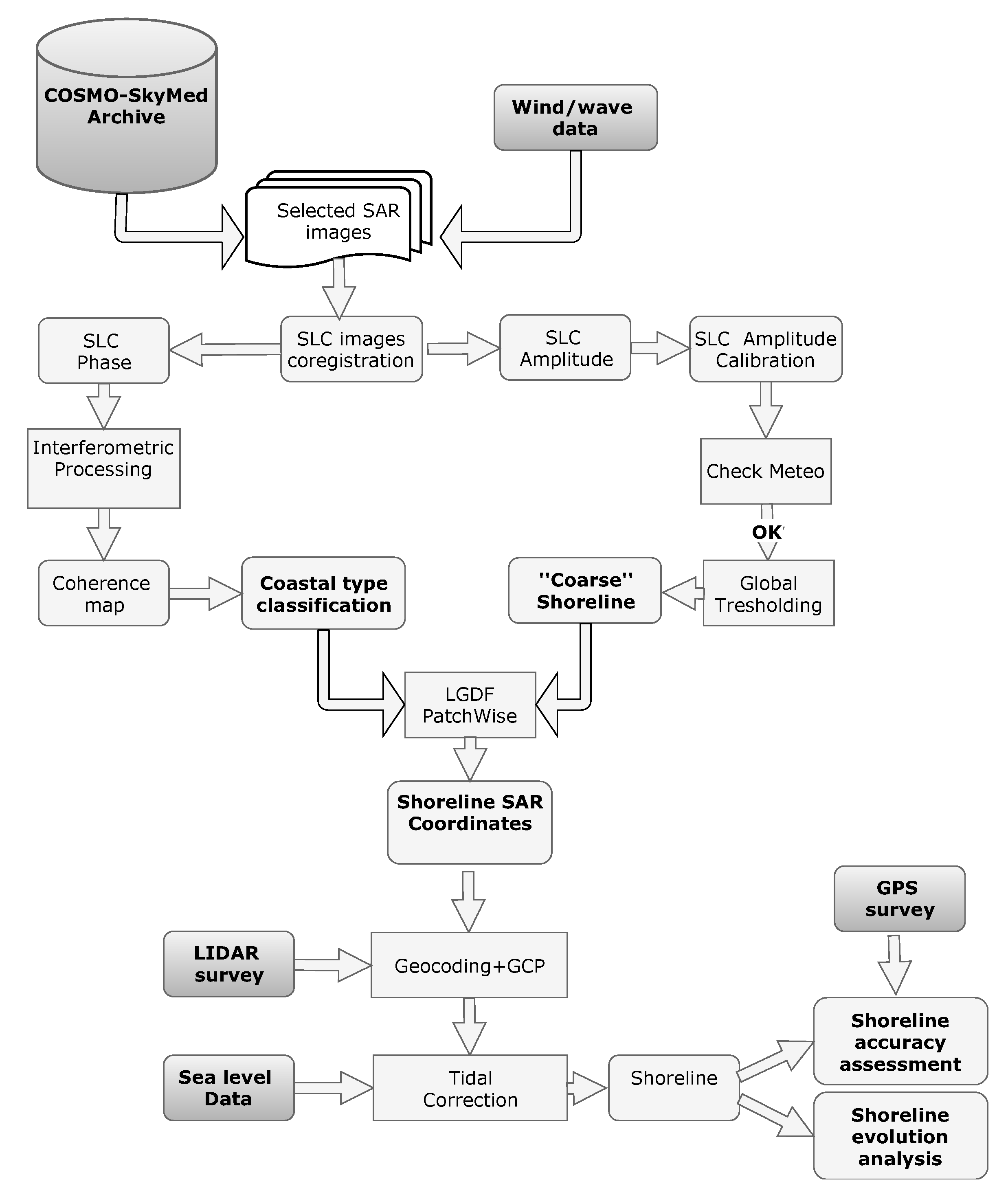
2. Methodology
2.1. Marine Weather Conditions
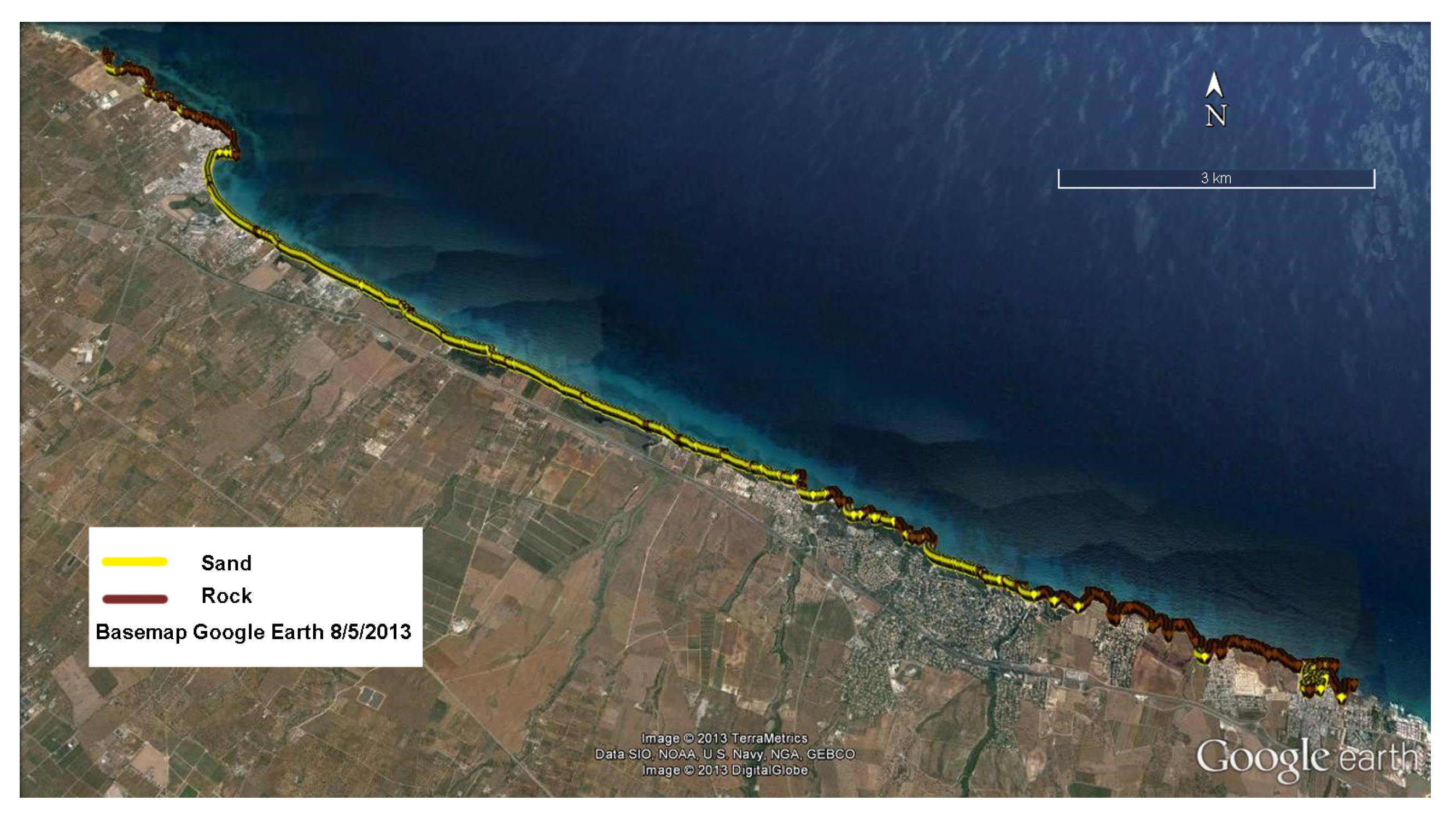
2.2. Coastal Type Classification
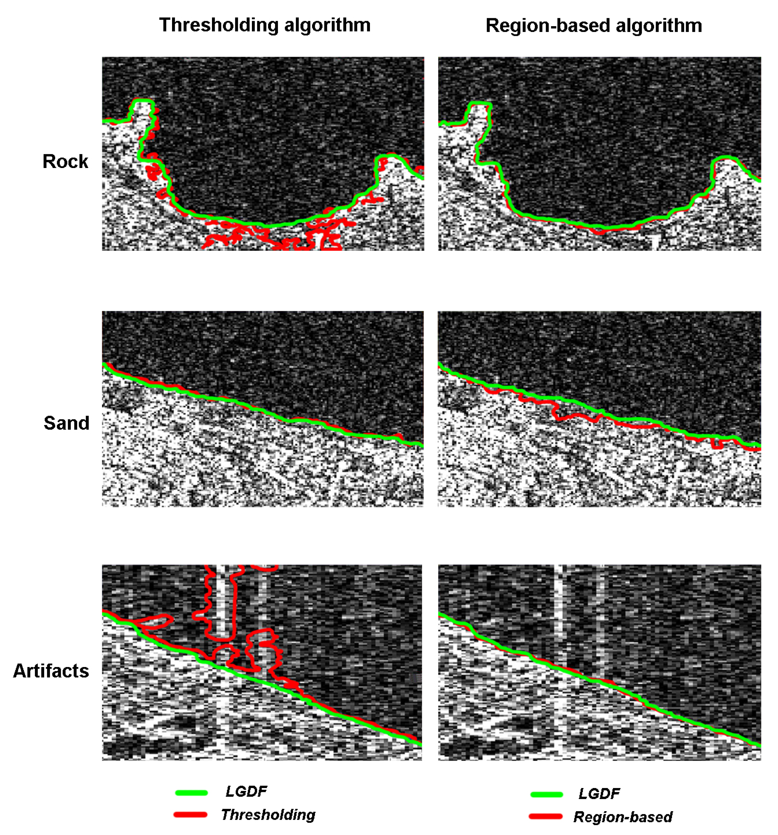
2.3. Land-Sea Interface Extraction
2.4. Precise Geocoding
2.5. Tidal Correction
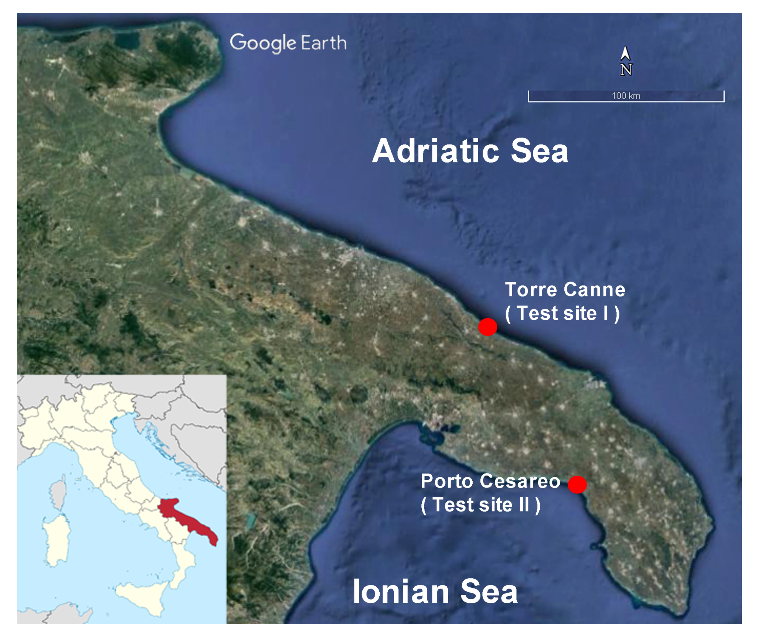
3. Case Studies
4. Results
5. Discussion
6. Conclusions
Author Contributions
Funding
Acknowledgments
Conflicts of Interest
References
- Pauli, G. The Blue Economy: 10 Years, 100 Innovations, 100 Million Jobs; Paradigm Publications: London, UK, 2010. [Google Scholar]
- Clark, J.R. Coastal Zone Management Handbook; CRC Press: Boca Raton, FL, USA, 2018. [Google Scholar]
- Di Risio, M.; Bruschi, A.; Lisi, I.; Pesarino, V.; Pasquali, D. Comparative Analysis of Coastal Flooding Vulnerability and Hazard Assessment at National Scale. J. Mar. Sci. Eng. 2017, 5, 51. [Google Scholar] [CrossRef]
- Nicholls, R.J.; Woodroffe, C.; Burkett, V. Chapter 20—Coastline Degradation as an Indicator of Global Change. In Climate Change, 2nd ed.; Letcher, T.M., Ed.; Elsevier: Boston, MA, USA, 2016; pp. 309–324. [Google Scholar]
- Furmańczyk, K.; Andrzejewski, P.; Benedyczak, R.; Bugajny, N.; Cieszyński, Ł; Dudzińska-Nowak, J.; Giza, A.; Paprotny, D.; Terefenko, P.; Zawiślak, T. Recording of selected effects and hazards caused by current and expected storm events in the Baltic Sea coastal zone. J. Coast. Res. 2014, 70, 338–342. [Google Scholar]
- Baart, F.; van der Kaaij, T.; van Ormondt, M.; van Dongeren, A.; van Koningsveld, M.; Roelvink, J.A. Real-time forecasting of morphological storm impacts: A case study in the Netherlands. J. Coast. Res. 2009, SI 54, 1617–1621. [Google Scholar]
- Anastasiou, S.; Sylaios, G. Assessment of Shoreline Changes and Evaluation of Coastal Protection Methods to Mitigate Erosion. Coast. Eng. J. 2016, 58, 1650006. [Google Scholar] [CrossRef]
- Deng, J.; Harff, J.; Zhang, W.; Schneider, R.; Dudzińska-Nowak, J.; Giza, A.; Terefenko, P.; Furmańczyk, K. The dynamic equilibrium shore model for the reconstruction and future projection of coastal morphodynamics. In Coastline Changes of the Baltic Sea from South to East; Springer: Berlin, Germany, 2017; pp. 87–106. [Google Scholar]
- Paprotny, D.; Andrzejewski, P.; Terefenko, P.; Furmańczyk, K. Application of empirical wave run-up formulas to the Polish Baltic Sea coast. PLoS ONE 2014, 9, e105437. [Google Scholar] [CrossRef] [PubMed]
- Roelvink, D.; Reniers, A.; Van Dongeren, A.; de Vries, J.v.T.; McCall, R.; Lescinski, J. Modelling storm impacts on beaches, dunes and barrier islands. Coast. Eng. 2009, 56, 1133–1152. [Google Scholar] [CrossRef]
- Enríquez, A.R.; Marcos, M.; Álvarez-Ellacuría, A.; Orfila, A.; Gomis, D. Changes in beach shoreline due to sea level rise and waves under climate change scenarios: Application to the Balearic Islands (western Mediterranean). Nat. Hazards Earth Syst. Sci. 2017, 17, 1075–1089. [Google Scholar] [CrossRef]
- Robinet, A.; Castelle, B.; Idier, D.; Le Cozannet, G.; Déqué, M.; Charles, E. Statistical modeling of interannual shoreline change driven by North Atlantic climate variability spanning 2000–2014 in the Bay of Biscay. Geo-Mar. Lett. 2016, 36, 479–490. [Google Scholar] [CrossRef] [Green Version]
- Dolan, R.; Hayden, B.P.; May, P.; May, S. The reliability of shoreline change measurements from aerial photographs. Shore Beach 1980, 48, 22–29. [Google Scholar]
- Lisi, I.; Molfetta, M.G.; Bruno, M.F.; Risio, M.D.; Damiani, L. Morphodynamic classification of sandy beaches in enclosed basins: The case study of Alimini (Italy). J. Coast. Res. 2011, SI 64, 180–184. [Google Scholar]
- Armenio, E.; Meftah, M.B.; Bruno, M.; De Padova, D.; De Pascalis, F.; De Serio, F.; Di Bernardino, A.; Mossa, M.; Leuzzi, G.; Monti, P. Semi enclosed basin monitoring and analysis of meteo, wave, tide and current data: Sea monitoring. In Proceedings of the 2016 IEEE Workshop on Environmental, Energy, and Structural Monitoring Systems (EESMS), Bari, Italy, 13–14 June 2016; pp. 1–6. [Google Scholar]
- Damiani, L.; Saponieri, A.; Valentini, N. Validation of swash model for run-up prediction on a natural embayed beach. Ital. J. Eng. Geol. Environ. 2018, SI 1, 27–37. [Google Scholar]
- Morton, R.A.; Leach, M.P.; Paine, J.G.; Cardoza, M.A. Monitoring Beach Changes Using GPS Surveying Techniques. J. Coast. Res. 1993, 9, 702–720. [Google Scholar]
- Kostrzewski, A.; Zwoliński, Z.; Winowski, M.; Tylkowski, J.; Samołyk, M. Cliff top recession rate and cliff hazards for the sea coast of Wolin Island (Southern Baltic). Baltica 2015, 28, 109–120. [Google Scholar] [CrossRef] [Green Version]
- Gens, R. Remote sensing of coastlines: Detection, extraction and monitoring. Int. J. Remote Sens. 2010, 31, 1819–1836. [Google Scholar] [CrossRef]
- Stockdon, H.F.; Sallenger, A.H., Jr.; List, J.H.; Holman, R.A. Estimation of Shoreline Position and Change Using Airborne Topographic Lidar Data. J. Coast. Res. 2002, 18, 502–513. [Google Scholar]
- Terefenko, P.; Zelaya Wziątek, D.; Dalyot, S.; Boski, T.; Pinheiro Lima-Filho, F. A High-Precision LiDAR-Based Method for Surveying and Classifying Coastal Notches. ISPRS Int. J. Geo-Inf. 2018, 7, 295. [Google Scholar] [CrossRef]
- Pereira, E.; Bencatel, R.; Correia, J.; Félix, L.; Gonçalves, G.; Morgado, J.; Sousa, J. Unmanned air vehicles for coastal and environmental research. J. Coast. Res. 2009, SI 54, 1557–1561. [Google Scholar]
- Mancini, F.; Dubbini, M.; Gattelli, M.; Stecchi, F.; Fabbri, S.; Gabbianelli, G. Using Unmanned Aerial Vehicles (UAV) for High-Resolution Reconstruction of Topography: The Structure from Motion Approach on Coastal Environments. Remote Sens. 2013, 5, 6880–6898. [Google Scholar] [CrossRef] [Green Version]
- Gonçalves, J.; Henriques, R. UAV photogrammetry for topographic monitoring of coastal areas. ISPRS J. Photogramm. Remote Sens. 2015, 104, 101–111. [Google Scholar] [CrossRef]
- Turner, I.L.; Harley, M.D.; Drummond, C.D. UAVs for coastal surveying. Coast. Eng. 2016, 114, 19–24. [Google Scholar] [CrossRef]
- Holman, R.A.; Stanley, J. The history and technical capabilities of Argus. Coast. Eng. 2007, 54, 477–491. [Google Scholar] [CrossRef]
- Archetti, R.; Paci, A.; Carniel, S.; Bonaldo, D. Optimal index related to the shoreline dynamics during a storm: the case of Jesolo beach. Nat. Hazards Earth Syst. Sci. 2016, 16, 1107–1122. [Google Scholar] [CrossRef] [Green Version]
- Valentini, N.; Saponieri, A.; Molfetta, M.G.; Damiani, L. New algorithms for shoreline monitoring from coastal video systems. Earth Sci. Informat. 2017, 10, 495–506. [Google Scholar] [CrossRef]
- Valentini, N.; Saponieri, A.; Damiani, L. A new video monitoring system in support of Coastal Zone Management at Apulia Region, Italy. Ocean Coast. Manag. 2017, 142, 122–135. [Google Scholar] [CrossRef]
- Cracknell, A. Remote sensing techniques in estuaries and coastal zones an update. Int. J. Remote Sens. 1999, 20, 485–496. [Google Scholar] [CrossRef]
- Richards, J.; Jia, X. Remote Sensing Digital Image Analysis; Springer: Berlin, Germany, 1999. [Google Scholar]
- Virelli, M.; Coletta, A.; Battagliere, M.L. ASI COSMO-SkyMed: Mission Overview and Data Exploitation. IEEE Geosci. Remote Sens. Mag. 2014, 2, 64–66. [Google Scholar] [CrossRef]
- Lee, J.S.; Jurkevich, I. Coastline Detection And Tracing In SAr Images. IEEE Trans. Geosci. Remote Sens. 1990, 28, 662–668. [Google Scholar] [Green Version]
- Bijaoui, J.; Cauneau, F. Separation of sea and land in SAR images using texture classification. In Proceedings of the OCEANS ’94. ’Oceans Engineering for Today’s Technology and Tomorrow’s Preservation, Brest, France, 13–16 September 1994; Volume 1, pp. I/522–I/526. [Google Scholar]
- Niedermeier, A.; Hoja, D.; Lehner, S. Topography and morphodynamics in the German Bight using SAR and optical remote sensing data. Ocean Dyn. 2005, 55, 100–109. [Google Scholar] [CrossRef] [Green Version]
- Liu, H.; Jezek, K. A complete high-resolution coastline of Antarctica extracted from orthorectified Radarsat SAR imagery. Photogramm. Eng. Remote Sens. 2004, 70, 605–616. [Google Scholar] [CrossRef]
- Wang, Z.; Yang, S.; Chen, T. Coastline extraction from tandem ERS 1/2 interferometric coherence map. In Proceedings of the 2012 International Workshop on Image Processing and Optical Engineering. International Society for Optics and Photonics, Harbin, China, 9–10 January 2012; p. 83351L. [Google Scholar]
- Dellepiane, S.; De Laurentiis, R.; Giordano, F. Coastline extraction from SAR images and a method for the evaluation of the coastline precision. Pattern Recogn. Lett. 2004, 25, 1461–1470. [Google Scholar] [CrossRef]
- Mason, D.; Davenport, I. Accurate and efficient determination of the shoreline in ERS-1 SAR images. IEEE Trans. Geosci. Remote Sens. 1996, 34, 1243–1253. [Google Scholar] [CrossRef]
- Modava, M.; Akbarizadeh, G. Coastline extraction from SAR images using spatial fuzzy clustering and the active contour method. Int. J. Remote Sens. 2016, 38, 355–370. [Google Scholar] [CrossRef]
- Osher, S.; Sethian, J.A. Fronts propagating with curvature-dependent speed: Algorithms based on Hamilton-Jacobi formulations. J. Comput. Phys. 1988, 79, 12–49. [Google Scholar] [CrossRef] [Green Version]
- Shu, Y.; Li, J.; Gomes, G. Shoreline extraction from RADARSAT-2 intensity imagery using a narrow band level set segmentation approach. Mar. Geod. 2010, 33, 187–203. [Google Scholar] [CrossRef]
- Ouyang, Y.; Chong, J.; Wu, Y. Two coastline detection methods in Synthetic Aperture Radar imagery based on Level Set Algorithm. Int. J. Remote Sens. 2010, 31, 4957–4968. [Google Scholar] [CrossRef]
- Zhao, L.; Fan, L.; Wang, C.; Tang, Y.; Zhang, B. A non-supervised method for shoreline extraction using high resolution SAR image. In Proceedings of the 2012 International Conference on Computer Vision in Remote Sensing (CVRS), Xiamen, China, 16–18 December 2012; pp. 317–322. [Google Scholar]
- Sheng, G.; Yang, W.; Deng, X.; He, C.; Cao, Y.; Sun, H. Coastline Detection in Synthetic Aperture Radar (SAR) Images by Integrating Watershed Transformation and Controllable Gradient Vector Flow (GVF) Snake Model. IEEE J. Ocean. Eng. 2012, 37, 375–383. [Google Scholar] [CrossRef]
- Palazzo, F.; Latini, D.; Baiocchi, V.; Del Frate, F.; Giannone, F.; Dominici, D.; Remondiere, S. An application of COSMO-SkyMed to coastal erosion studies. Eur. J. Remote Sens. 2012, 45, 361–370. [Google Scholar] [CrossRef]
- Braga, F.; Tosi, L.; Prati, C.; Alberotanza, L. Shoreline detection: Capability of COSMO-SkyMed and high-resolution multispectral images. Eur. J. Remote Sens. 2013, 46, 837–853. [Google Scholar] [CrossRef]
- Baselice, F.; Ferraioli, G.; Pascazio, V. Coastal line extraction from SAR multi-channel images. In Proceedings of the 2012 Tyrrhenian Workshop on Advances in Radar and Remote Sensing (TyWRRS), Naples, Italy, 12–14 September 2012; pp. 322–325. [Google Scholar]
- Nunziata, F.; Migliaccio, M.; Li, X. Dual-polarized COSMO-SkyMed SAR data for coastline detection. In Proceedings of the 2012 IEEE International on Geoscience and Remote Sensing Symposium (IGARSS), Munich, Germany, 22–27 July 2012; pp. 5109–5112. [Google Scholar]
- Nunziata, F.; Migliaccio, M.; Li, X.; Ding, X. Coastline extraction using dual-polarimetric COSMO-SkyMed PingPong mode SAR data. IEEE Geosci. Remote Sens. Lett. 2014, 11, 104–108. [Google Scholar] [CrossRef]
- Nunziata, F.; Buono, A.; Migliaccio, M.; Benassai, G. Dual-polarimetric C-and X-band SAR data for coastline extraction. IEEE J. Sel. Top. Appl. Earth Observ. Remote Sens. 2016, 9, 4921–4928. [Google Scholar] [CrossRef]
- De Laurentiis, L.; Latini, D.; Del Frate, F.; Schiavon, G. Automatic procedure for coastline extraction exploiting full-pol SAR imagery and AANN-PCNN processing chain. Proc. SPIE 2018, 10789, 10789. [Google Scholar]
- Bruno, M.F.; Molfetta, M.G.; Pratola, L.; Mossa, M.; Nutricato, R.; Morea, A.; Nitti, d.O.; Teresa, C.M. Remote Sensed and In Situ Data: An integrated approach for Coastal Risk Assessment. In Proceedings of the International Workshop on Metrology for the Sea (MetroSea 2018), Bari, Italy, 8–10 October 2018; pp. 13–17. [Google Scholar]
- Lee, J.S. Speckle analysis and smoothing of synthetic aperture radar images. Comput. Graph. Image Process. 1981, 17, 24–32. [Google Scholar] [CrossRef]
- Otsu, N. A threshold selection method from gray-level histograms. Automatica 1975, 11, 23–27. [Google Scholar] [CrossRef]
- Canny, J. A computational approach to edge detection. IEEE Trans. Pattern Anal. Mach. Intell. 1986, PAMI-8, 679–698. [Google Scholar] [CrossRef]
- Wang, L.; He, L.; Mishra, A.; Li, C. Active contours driven by local Gaussian distribution fitting energy. Signal Process. 2009, 89, 2435–2447. [Google Scholar] [CrossRef]
- Bruno, M.F.; Molfetta, M.G.; Mossa, M.; Morea, A.; Chiaradia, M.T.; Nutricato, R.; Nitti, D.O.; Guerriero, L.; Coletta, A. Integration of multitemporal SAR/InSAR techniques and NWM for coastal structures monitoring: Outline of the software system and of an operational service with COSMO-SkyMed data. In Proceedings of the 2016 IEEE Workshop on Environmental, Energy, and Structural Monitoring Systems (EESMS), Bari, Italy, 13–14 June 2016; pp. 1–6. [Google Scholar]
- Bruno, M.F.; Molfetta, M.G.; Mossa, M.; Nutricato, R.; Morea, A.; Chiaradia, M.T. Coastal Observation through Cosmo-SkyMed High-Resolution SAR Images. J. Coast. Res. 2016, 75, 795–799. [Google Scholar] [CrossRef]
- Bovenga, F.; Refice, A.; Nutricato, R.; Guerriero, L.; Chiaradia, M. SPINUA: A flexible processing chain for ERS/ENVISAT long term interferometry. In Proceedings of the ESA-ENVISAT Symposium, Salzburg, Austria, 6–10 September 2004; pp. 6–10. [Google Scholar]
- Wu, L.; Tajima, Y.; Yamanaka, Y.; Shimozono, T.; Sato, S. Study on characteristics of synthetic aperture radar (SAR) imagery around the coast for shoreline detection. Coast. Eng. J. 2018, 1–19. [Google Scholar] [CrossRef]
- Hasselmann, S.; Brüning, C.; Hasselmann, K.; Heimbach, P. An improved algorithm for the retrieval of ocean wave spectra from synthetic aperture radar image spectra. J. Geophys. Res. 1996, 101, 16615–16629. [Google Scholar] [CrossRef]
- Rana, F.M.; Adamo, M.; Pasquariello, G.; De Carolis, G.; Morelli, S.; Bovenga, F. A simplified local gradient method for the retrieval of SARderived sea surface wind directions. In Proceedings of the EUSAR 2014; 10th European Conference on Synthetic Aperture Radar, Berlin, Germany, 3–5 June 2014; pp. 1–4. [Google Scholar]
- Benassai, G.; Migliaccio, M.; Nunziata, F. The use of COSMO-SkyMed© SAR data for coastal management. J. Mar. Sci. Technol. 2015, 20, 542–550. [Google Scholar] [CrossRef]
- Nitti, D.O.; Hanssen, R.F.; Refice, A.; Bovenga, F.; Nutricato, R. Impact of DEM-assisted coregistration on high-resolution SAR interferometry. IEEE Trans. Geosci. Remote Sens. 2011, 49, 1127–1143. [Google Scholar] [CrossRef]
- Locorotondo, P.; Guerriero, A.; Chiaradia, M.T.; Nitti, D.O.; Nutricato, R.; Bovenga, F. Preliminary assessment of side-lobe mitigation techniques for proper coherent targets selection in MTInSAR applications. In Proceedings of the Active and Passive Microwave Remote Sensing for Environmental Monitoring II, Berlin, Germany, 12 September 2018; Volume 10788, p. 1078804. [Google Scholar]
- Nitti, D.O.; Bovenga, F.; Nutricato, R.; Refice, A.; Bruno, M.F.; Petrillo, A.F.; Chiaradia, M.T. On the use of Numerical Weather Models for improving SAR geolocation accuracy. In Proceedings of the EUSAR 2014; 10th European Conference on Synthetic Aperture Radar, Berlin, Germany, 3–5 June 2014; pp. 1–4. [Google Scholar]
- Nitti, D.O.; Nutricato, R.; Lorusso, R.; Lombardi, N.; Bovenga, F.; Bruno, M.F.; Chiaradia, M.T.; Milillo, G. On the geolocation accuracy of COSMO-SkyMed products. In Proceedings of the SAR Image Analysis, Modeling, and Techniques XV, Toulouse, France, 21–24 September 2015; Volume 9642, p. 96420D. [Google Scholar]
- National Imagery and Mapping Agency. High Resolution Terrain Information (HRTI): Performance Specification; Technical Report; NIMA: Springfield, VA, USA, 2000.
- Damiani, L.; Bruno, M.F.; Molfetta, M.G.; Nobile, B. Coastal zone monitoring in Apulia region: First analysis on meteomarine climate. In Proceedings of the Vth International Symposium on Environmental Hydraulics (ISEH 2007), Tempe, AZ, USA, 4–7 December 2007. [Google Scholar]
- Bruno, M.F.; Molfetta, M.G.; Petrillo, A.F. The influence of interannual variability of mean sea level in the Adriatic Sea on extreme values. J. Coast. Res. 2014, 241–246. [Google Scholar] [CrossRef]
- Pasquali, D.; Bruno, M.; Celli, D.; Damiani, L.; Risio, M.D. A simplified hindcast method for the estimation of extreme storm surge events in semi-enclosed basins. Appl. Ocean Res. 2019, 85, 45–52. [Google Scholar] [CrossRef]
- Bencivenga, M.; Nardone, G.; Ruggiero, F.; Calore, D. The Italian data buoy network (RON). Adv. Fluid Mech. IX 2012, 74, 321. [Google Scholar]
- Dee, D.P.; Uppala, S.; Simmons, A.; Berrisford, P.; Poli, P.; Kobayashi, S.; Andrae, U.; Balmaseda, M.; Balsamo, G.; Bauer, P.; et al. The ERA-Interim reanalysis: Configuration and performance of the data assimilation system. Q. J. R. Meteorol. Soc. 2011, 137, 553–597. [Google Scholar] [CrossRef]
- Infoterra. Radiometric Calibration of TerraSAR-X Data; Technical Report; Infoterra: Friedrichshafen, Germany, 2008. [Google Scholar]
- Mitra, S.S.; Mitra, D.; Santra, A. Performance testing of selected automated coastline detection techniques applied on multispectral satellite imageries. Earth Sci. Informat. 2017, 10, 321–330. [Google Scholar] [CrossRef]
- Modava, M.; Akbarizadeh, G.; Soroosh, M. Integration of spectral histogram and level set for coastline detection in SAR images. IEEE Trans. Aerosp. Electron. Syst. 2018. [Google Scholar] [CrossRef]
- Vandebroek, E.; Lindenbergh, R.; van Leijen, F.; de Schipper, M.; de Vries, S.; Hanssen, R. Semi-automated monitoring of a mega-scale beach nourishment using high-resolution terrasar-x satellite data. Remote Sens. 2017, 9, 653. [Google Scholar] [CrossRef]
- Yoon, Y.T.; Eineder, M.; Yague-Martinez, N.; Montenbruck, O. TerraSAR-X precise trajectory estimation and quality assessment. IEEE Trans. Geosci. Remote Sens. 2009, 47, 1859–1868. [Google Scholar] [CrossRef]
- Eineder, M.; Minet, C.; Steigenberger, P.; Cong, X.; Fritz, T. Imaging geodesy—Toward centimeter-level ranging accuracy with TerraSAR-X. IEEE Trans. Geosci. Remote Sens. 2011, 49, 661–671. [Google Scholar] [CrossRef]


| Test Site I | Test Site II | |
|---|---|---|
| SAR dataset | 19 CSK Stripmap HIMAGE | 38 CSK Stripmap HIMAGE |
| DEM | LIDAR DEM 2008 1 m | LIDAR DEM 2008 1 m |
| (POR PUGLIA 2000–2006) | (POR PUGLIA 2000–2006) | |
| Aerial photos | Maritime State Office (Apulia Region) | Maritime State Office (Apulia Region) |
| Waves | RON Wave Buoy (Monopoli) | SIMOP Wave Buoy (Taranto) |
| Tides | RMN Tidal station (Bari) | SIMOP Tidal station (Porto Cesareo) |
| GPS survey | 60 GPS transects spaced 10 m | 50 GPS transects spaced 10 m |
| CSK_H4-05_HH_RD_009 | CSK_H4-01_HH_RA_009 | CSK_H4-02_HH_RA_009 | |
|---|---|---|---|
| Instrument Mode | STR_HIMAGE | STR_HIMAGE | STR_HIMAGE |
| Polarization | HH | HH | HH |
| Look Side | right | right | right |
| Pass Direction | D | A | A |
| Track | 9 | 209 | 209 |
| Beam ID | H4-05 | H4-01 | H4-02 |
| Off Nadir Angle | 30620 | 24130 | 24670 |
| Satellite ID | SAR1 | SAR1 | SAR1 |
| Algorithm | Rocky Coast | Sandy Coast | Artifact |
|---|---|---|---|
| Thresholding | GOOD | GOOD | POOR |
| Region-based | GOOD | POOR | GOOD |
| LGDF | GOOD | GOOD | GOOD |
| Test Site | Mean (m) | Standard Deviation (m) | RMSE (m) |
|---|---|---|---|
| Test Site I | 1.12 | 0.78 | 1.35 |
| Test Site II | 1.36 | 1.47 | 2.2 |
| Accuracy | |||
|---|---|---|---|
| Test Site | <1 Pixel Distance | 1–2 Pixel Distance | 2–3 Pixel Distance |
| Test Site I | 87% | 100% | 100% |
| Test Site II | 85% | 98% | 100% |
© 2019 by the authors. Licensee MDPI, Basel, Switzerland. This article is an open access article distributed under the terms and conditions of the Creative Commons Attribution (CC BY) license (http://creativecommons.org/licenses/by/4.0/).
Share and Cite
Bruno, M.F.; Molfetta, M.G.; Pratola, L.; Mossa, M.; Nutricato, R.; Morea, A.; Nitti, D.O.; Chiaradia, M.T. A Combined Approach of Field Data and Earth Observation for Coastal Risk Assessment. Sensors 2019, 19, 1399. https://doi.org/10.3390/s19061399
Bruno MF, Molfetta MG, Pratola L, Mossa M, Nutricato R, Morea A, Nitti DO, Chiaradia MT. A Combined Approach of Field Data and Earth Observation for Coastal Risk Assessment. Sensors. 2019; 19(6):1399. https://doi.org/10.3390/s19061399
Chicago/Turabian StyleBruno, Maria Francesca, Matteo Gianluca Molfetta, Luigi Pratola, Michele Mossa, Raffaele Nutricato, Alberto Morea, Davide Oscar Nitti, and Maria Teresa Chiaradia. 2019. "A Combined Approach of Field Data and Earth Observation for Coastal Risk Assessment" Sensors 19, no. 6: 1399. https://doi.org/10.3390/s19061399