Adaptive Phase Transform Method for Pipeline Leakage Detection

Abstract
:1. Introduction
2. Methodology
2.1. Water Leak Detection
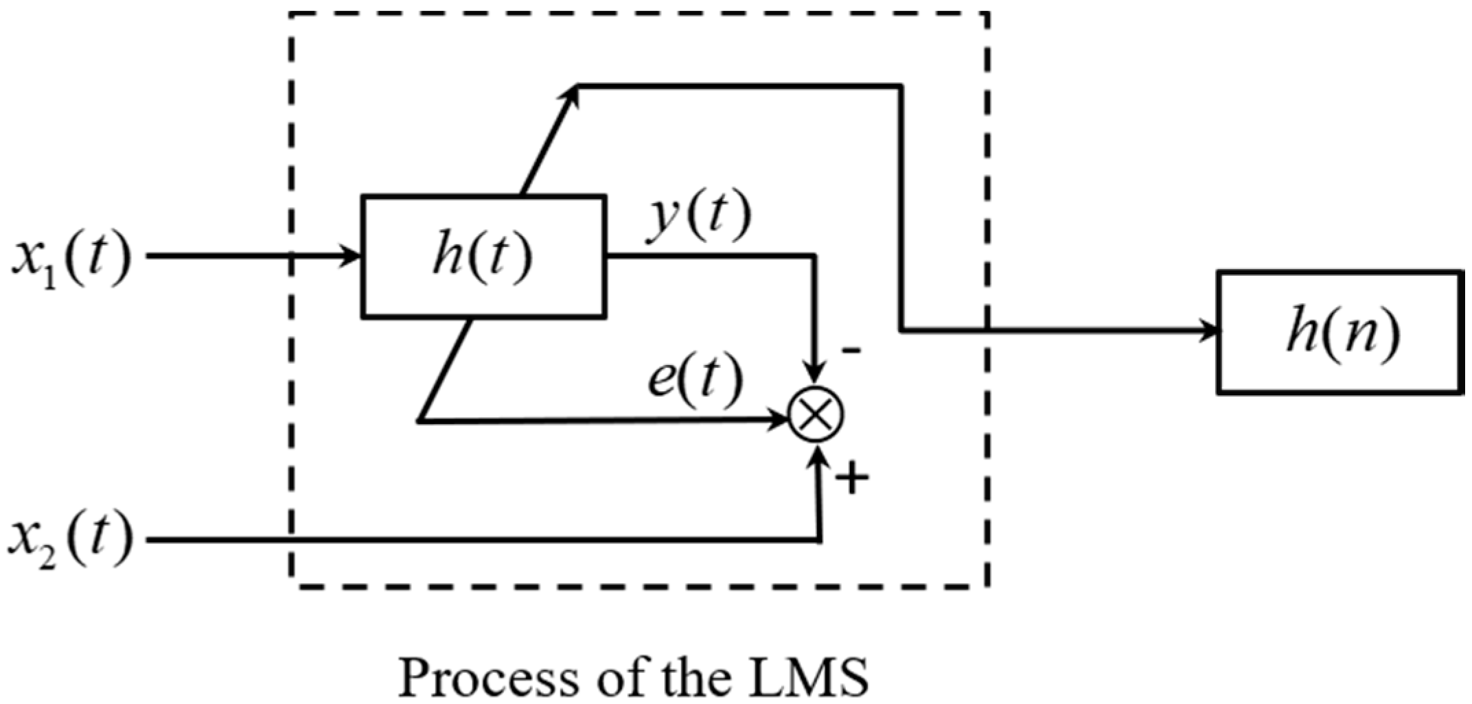
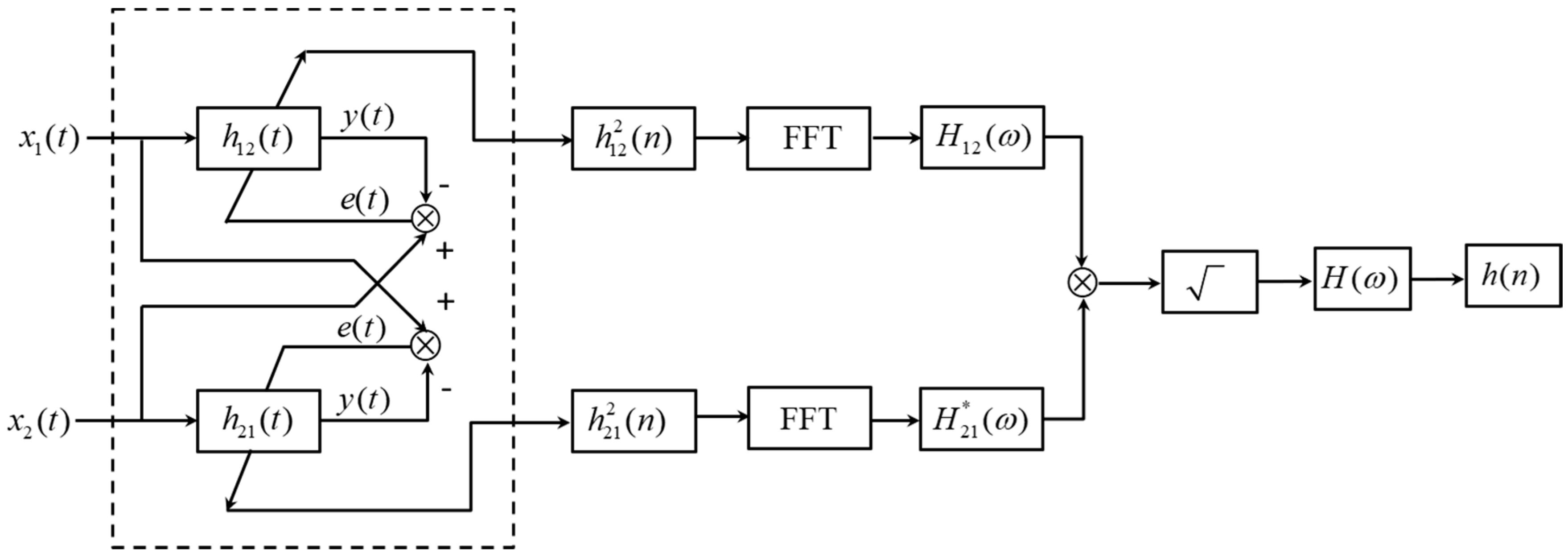
2.2. The Proposed ADPHAT Method
- (1)
- If there is no time delay between two signals x1(t) and x2(t) (i.e., T0 = 0), then the maximum value of the IRF h(n) occurs at n = 0. Setting n = 0, Equation (9) leads to the two FRFs given byIt is clear from Equation (10) that when T0 = 0, the gradient of the phase spectrum is −P/fs, which is defined as the reference time delay, Tref, by
- (2)
- When the time delay , FTs of the two IRFs lead toFrom Equations (12a) and (12b), the phase spectra between two sensor signals can be obtained by
2.3. Improvement in TDE
3. Numerical Examples
4. Experimental Work
4.1. Case One
4.2. Case Two
5. Conclusions
Author Contributions
Funding
Conflicts of Interest
Nomenclature
| d1, d2 | distances between the leak and sensors 1 and 2 |
| D | distance between two sensors |
| B | fluid bulk modulus |
| E | Young’s modulus of the pipe wall |
| a, h | pipe radius and wall thickness |
| β | wave attenuation factor |
| k, kf | fluid-borne wavenumber and free-field fluid wavenumber |
| T0 | estimate of the time delay |
| η | loss factor of the pipe wall |
| c, cf | propagation and fluid wavespeeds |
| x1(t), x2(t) | leak signals measured |
| l(t) | leak source signal |
| n1(t), n2(t) | background noise |
| H(ω,d1), H(ω,d2) | FRFs between l(t) and x1(t), x2(t) |
| h1(t), h2(t) | IRFs between l(t) and x1(t), x2(t) |
| S12(ω) | CSD between x1(t) and x2(t) |
| Φ12(ω), Φ21(ω) | phase spectra of x1(t) and x2(t) |
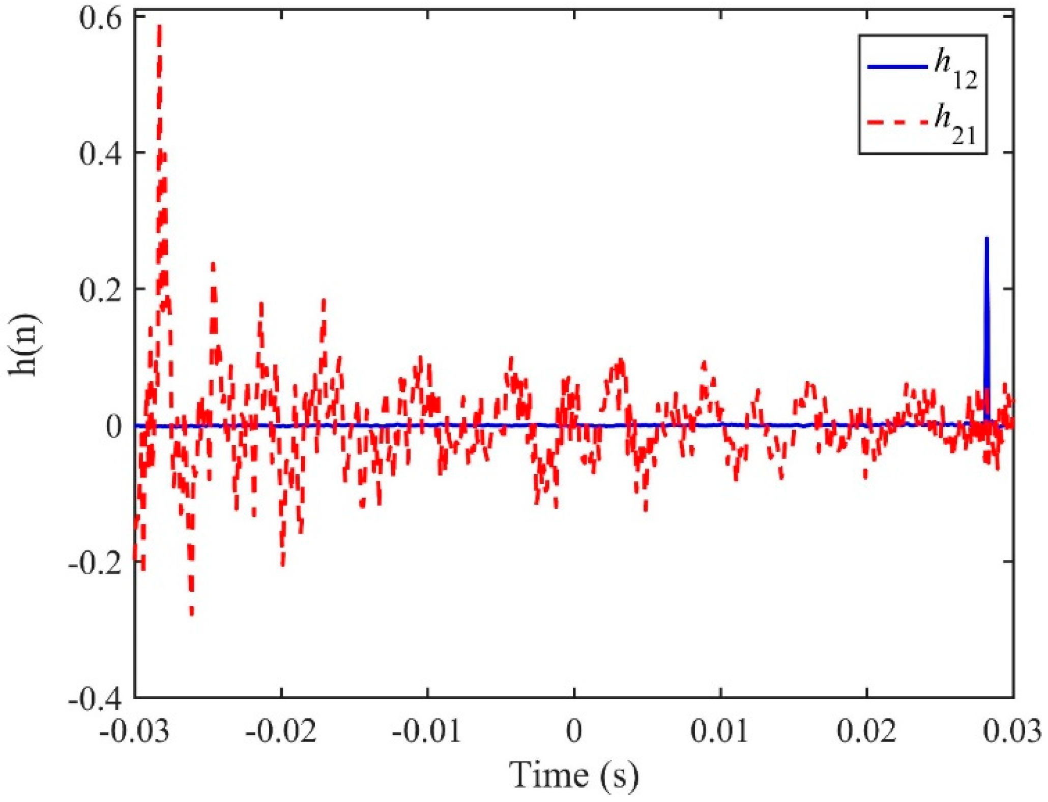
| h21(n), h12(n), h(n) | IRFs for measured signals |
| H(ω), H12(ω), H21(ω) | FTs of h12(n), h21(n), h(n) |
| Tref | reference time delay |
| λmax | maximum order in the LMS algorithm |
Appendix A. The LMS Adaptive Algorithm for TDE
References
- Ben-Mansour, R.; Habib, M.A.; Khalifa, A.; Youcef, K.T.; Chatzigeorgiou, D. Computational fluid dynamic simulation of small leaks in water pipelines for direct leak pressure transduction. Comput. Fluids 2012, 57, 110–123. [Google Scholar] [CrossRef]
- Li, H.; Zhang, P.; Song, G.; Patil, D.; Mo, Y. Robustness study of the pounding tuned mass damper for vibration control of subsea jumpers. Smart Mater. Struct. 2015, 24, 095001. [Google Scholar] [CrossRef]
- Kawsar, M.R.U.; Youssef, S.A.; Faisal, M.; Kumar, A.; Seo, J.K.; Paik, J.K. Assessment of dropped object risk on corroded subsea pipeline. Ocean Eng. 2015, 106, 329–340. [Google Scholar] [CrossRef]
- Farley, M.; Wyeth, G.; Ghazali, Z.B.M.; Istandar, A.; Singh, S. The Manager’s Non-Revenue Water Handbook: A Guide to Understanding Water Losses; Ranhill Utilities Berhad and the United States Agency for International Development: Bangkok, Thailand, 2008. [Google Scholar]
- China Statistical Yearbook. 2017. Available online: www.stats.gov.cn/tjsj/ndsj/2017/indexeh.htm (accessed on 1 May 2018).
- International Decade for Action ‘WATER FOR LIFE’ 2005–2015. 2015. Available online: www.un.org/waterforlifedecade/scarcity.shtml (accessed on 1 May 2018).
- Andersen, J.H.; Powell, R.S. Implicit state-estimation technique for water network monitoring. Urban Water 2000, 2, 123–130. [Google Scholar] [CrossRef]
- Poulakis, Z.; Valougeorgis, D.; Papadimitriou, C. Leakage detection in water pipe networks using a Bayesian probabilistic framework. Probab. Eng. Mech. 2003, 18, 314–327. [Google Scholar] [CrossRef]
- Lee, P.J.; Vitkovsky, J.P.; Lambert, M.F.; Simpson, A.R.; Liggett, J.A. Leak location using the pattern of the frequency response diagram in pipelines: A numerical study. J. Sound Vib. 2005, 284, 1051–1073. [Google Scholar] [CrossRef]
- Lee, P.J.; Simpson, A.R.; Vitkovsky, J.P.; Liggett, J.A. Experimental verification of the frequency response method for pipeline leak detection. J. Hydraul. Res. 2006, 44, 693–707. [Google Scholar] [CrossRef] [Green Version]
- Huang, S.C.; Lin, W.W.; Tasi, M.T.; Chen, M.H. Fiber optic in-line distributed sensor for detection and localization of the pipeline leaks. Sens. Actuators A Phys. 2007, 135, 570–579. [Google Scholar] [CrossRef]
- Hiroki, S.; Tanzawa, S.; Arai, T.; Abe, T. Development of water leak detection method in fusion reactors using water-soluble gas. Fusion Eng. Des. 2008, 83, 72–78. [Google Scholar] [CrossRef]
- Colombo, A.F.; Lee, P.; Karney, B.W. A selective literature review of transient-based leak detection methods. J. Hydrol. Environ. Res. 2009, 2, 212–227. [Google Scholar] [CrossRef]
- Puust, R.; Kapelan, Z.; Savic, D.A.; Koppel, T. A review of methods for leakage management in pipe networks. Urban Water J. 2010, 7, 25–45. [Google Scholar] [CrossRef]
- Yan, S.Z.; Chyan, L.S. Performance enhancement of BOTDR fiber optic sensor for oil and gas pipeline monitoring. Opt. Fiber Technol. 2010, 16, 100–109. [Google Scholar] [CrossRef]
- Bedjaoui, N.; Weyer, E. Algorithms for leak detection, estimation, isolation and localization in open water channels. Control Eng. Pract. 2011, 19, 564–573. [Google Scholar] [CrossRef]
- Ghazali, M.F.; Beck, S.B.M.; Shucksmith, J.D.; Boxall, J.B.; Staszewski, W.J. Comparative study of instantaneous frequency based methods for leak detection in pipeline networks. Mech. Syst. Signal Process. 2012, 29, 187–200. [Google Scholar] [CrossRef] [Green Version]
- Ozevin, D.; Harding, J. Novel leak localization in pressurized pipeline networks using acoustic emission and geometric connectivity. Int. J. Pres. Ves. Pip. 2012, 92, 63–69. [Google Scholar] [CrossRef]
- Durocher, A.; Bruno, V.; Chantant, M.; Gargiulo, L.; Gherman, T.; Hatchressian, J.C.; Houry, M.; Le, R.; Mouyon, D. Remote leak localization approach for fusion machines. Fusion Eng. Des. 2013, 88, 1390–1394. [Google Scholar] [CrossRef]
- Mulholland, M.; Purdon, A.; Latifi, M.A.; Brouckaert, C.; Buckley, C. Leak identification in a water distribution network using sparse flow measurements. Comput. Chem. Eng. 2014, 66, 252–258. [Google Scholar] [CrossRef]
- Ni, L.; Jiang, J.C.; Pan, Y.; Wang, Z.R. Leak location of pipelines based on characteristic entropy. J. Loss Prev. Proc. 2014, 30, 24–36. [Google Scholar] [CrossRef]
- Lee, P.J.; Duan, H.F.; Tuck, J.; Ghidaoui, M. Numerical and Experimental Study on the Effect of Signal Bandwidth on Pipe Assessment Using Fluid Transients. J. Hydraul. Res. Int. J. Res. 2015, 141, 68–78. [Google Scholar] [CrossRef]
- Datta, S.; Sarkar, S. A review on different pipeline fault detection methods. J. Loss. Prev. Proc. 2016, 41, 97–106. [Google Scholar] [CrossRef]
- Guo, C.; Wen, Y.M.; Li, P.; Wen, J. Adaptive noise cancellation based on EMD in water-supply pipeline leak detection. Measurement 2016, 79, 188–197. [Google Scholar] [CrossRef]
- Lu, W.Q.; Liang, W.; Zhang, L.B.; Liu, W. A novel noise reduction method applied in negative pressure wave for pipeline leakage localization. Process. Saf. Environ. 2016, 104, 142–149. [Google Scholar] [CrossRef]
- Abdulshaheed, A.; Mustapha, F.; Ghavamian, A. A pressure-based method for monitoring leaks in a pipe distribution system: A Review. Renew. Sustain. Energy Rev. 2017, 69, 902–911. [Google Scholar] [CrossRef]
- Liu, C.; Li, Y.; Fang, L.; Xu, M. Experimental study on a de-noising system for gas and oil pipelines based on an acoustic leak detection and location method. Int. J. Pres. Vessels Pip. 2017, 151, 20–34. [Google Scholar] [CrossRef]
- Chehami, L.; Moulin, E.; Rosny, J.D.; Prada, C.; Chatelet, E. Nonlinear secondary noise sources for passive defect detection using ultrasound sensors. J. Sound Vib. 2017, 386, 283–294. [Google Scholar] [CrossRef]
- Nguyen, S.T.N.; Gong, J.Z.; Lambert, M.F.; Zecchin, A.C.; Simpson, A.R. Least squares deconvolution for leak detection with a pseudo random binary sequence excitation. Mech. Syst. Signal Process. 2018, 9, 846–858. [Google Scholar] [CrossRef]
- Zahab, S.E.; Abdelkader, E.M.; Zayed, T. An accelerometer-based leak detection system. Mech. Syst. Signal Process. 2018, 108, 276–291. [Google Scholar] [CrossRef]
- Fuchs, H.; Riehle, R. Ten years of experience with leak detection by acoustic signal analysis. Appl. Acoust. 1991, 33, 1–19. [Google Scholar] [CrossRef]
- Gao, Y.; Brennan, M.J.; Joseph, P.F. A comparison of time delay estimators for the detection of leak noise signals in plastic water distribution pipes. J. Sound Vib. 2006, 292, 552–570. [Google Scholar] [CrossRef]
- Knapp, C.; Carter, G. The generalized correlation method for estimation of time delay. IEEE Trans. Acous. Speech Signal Process. 1976, 24, 320–327. [Google Scholar] [CrossRef]
- Gao, Y.; Sui, F.S.; Muggleton, J.M.; Yang, J. Simplified dispersion relationships for fluid-dominated axisymmetric wave motion in buried fluid-filled pipes. J. Sound Vib. 2016, 375, 386–402. [Google Scholar] [CrossRef]
- Gao, Y.; Liu, Y.Y.; Ma, Y.F.; Cheng, X.B.; Yang, J. Application of the differentiation process into the correlation-based leak detection in urban pipeline networks. Mech. Syst. Signal Process. 2018, 112, 251–264. [Google Scholar] [CrossRef]
- Piersol, A. Time delay estimation using phase data. IEEE Trans. Acoust. Speech Signal Process. 1981, 29, 471–477. [Google Scholar] [CrossRef]
- Zhen, Z.; Hou, Z.Q. The generalized phase spectrum method for time delay estimation, in Acoustics, Speech, and Signal Processing. In Proceedings of the IEEE International Conference on ICASSP’84, San Diego, CA, USA, 19–21 March 1984. [Google Scholar]
- Brennan, M.J.; Gao, Y.; Joseph, P. On the relationship between time and frequency domain methods in time delay estimation for leak detection in water distribution pipes. J. Sound Vib. 2007, 304, 213–223. [Google Scholar] [CrossRef]
- Pinnington, R.; Briscoe, A. Externally applied sensor for axisymmetric waves in a fluid filled pipe. J. Sound Vib. 1994, 173, 503–516. [Google Scholar] [CrossRef]
- Behrouz, F.B. Adaptive Filters: Theory and Applications; John Wiley & Sons: New York, NY, USA, 2013. [Google Scholar]
- Widrow, B.; Glover, J.R.; McCool, J.M.; Kaunitz, J.; Williams, C.S.; Hearn, R.H.; Zeidler, J.R., Jr.; Dong, E.; Goodlin, R.C. Adaptive noise cancelling: Principles and applications. Proc. IEEE 1975, 63, 1692–1716. [Google Scholar] [CrossRef]


© 2019 by the authors. Licensee MDPI, Basel, Switzerland. This article is an open access article distributed under the terms and conditions of the Creative Commons Attribution (CC BY) license (http://creativecommons.org/licenses/by/4.0/).
Share and Cite
Ma, Y.; Gao, Y.; Cui, X.; Brennan, M.J.; Almeida, F.C.L.; Yang, J. Adaptive Phase Transform Method for Pipeline Leakage Detection. Sensors 2019, 19, 310. https://doi.org/10.3390/s19020310
Ma Y, Gao Y, Cui X, Brennan MJ, Almeida FCL, Yang J. Adaptive Phase Transform Method for Pipeline Leakage Detection. Sensors. 2019; 19(2):310. https://doi.org/10.3390/s19020310
Chicago/Turabian StyleMa, Yifan, Yan Gao, Xiwang Cui, Michael J. Brennan, Fabricio C.L. Almeida, and Jun Yang. 2019. "Adaptive Phase Transform Method for Pipeline Leakage Detection" Sensors 19, no. 2: 310. https://doi.org/10.3390/s19020310
APA StyleMa, Y., Gao, Y., Cui, X., Brennan, M. J., Almeida, F. C. L., & Yang, J. (2019). Adaptive Phase Transform Method for Pipeline Leakage Detection. Sensors, 19(2), 310. https://doi.org/10.3390/s19020310