Measurements of the Vertical Displacements of a Railway Bridge Using TLS Technology in the Context of the Upgrade of the Polish Railway Transport


Abstract
:1. Introduction
2. Materials and Methods
- the research object was specifically defined,
- the same variants of object monitoring were set during subsequent periodic measurements,
- measurement methods and measurement technologies were set that would be sufficiently accurate, and
- a research schedule was set to ensure timely periodic measurements (according to [43]).
2.1. Object
2.2. The Concept of Object Measurement
2.3. Procedures for Determining the Optimal Post-Processing of 3D Data
- —differences in the displacement values of the single node () of the main girders,
- —vertical displacements of the single node () of the main girders determined by leveling,
- —vertical displacements of the single node () of the main girders determined by TLS.
3. Results and Discussion
3.1. TLS Data Post-Processing
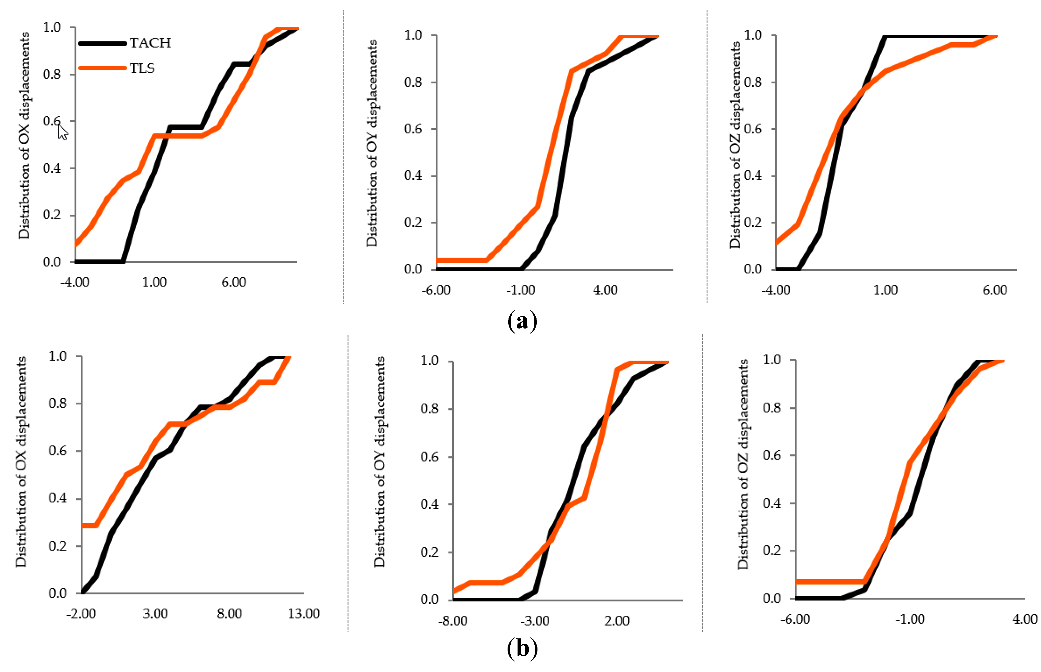
3.2. Case Study 1—Controlled Point Network Analysis
3.3. Case Study 2—Point Clouds Analysis
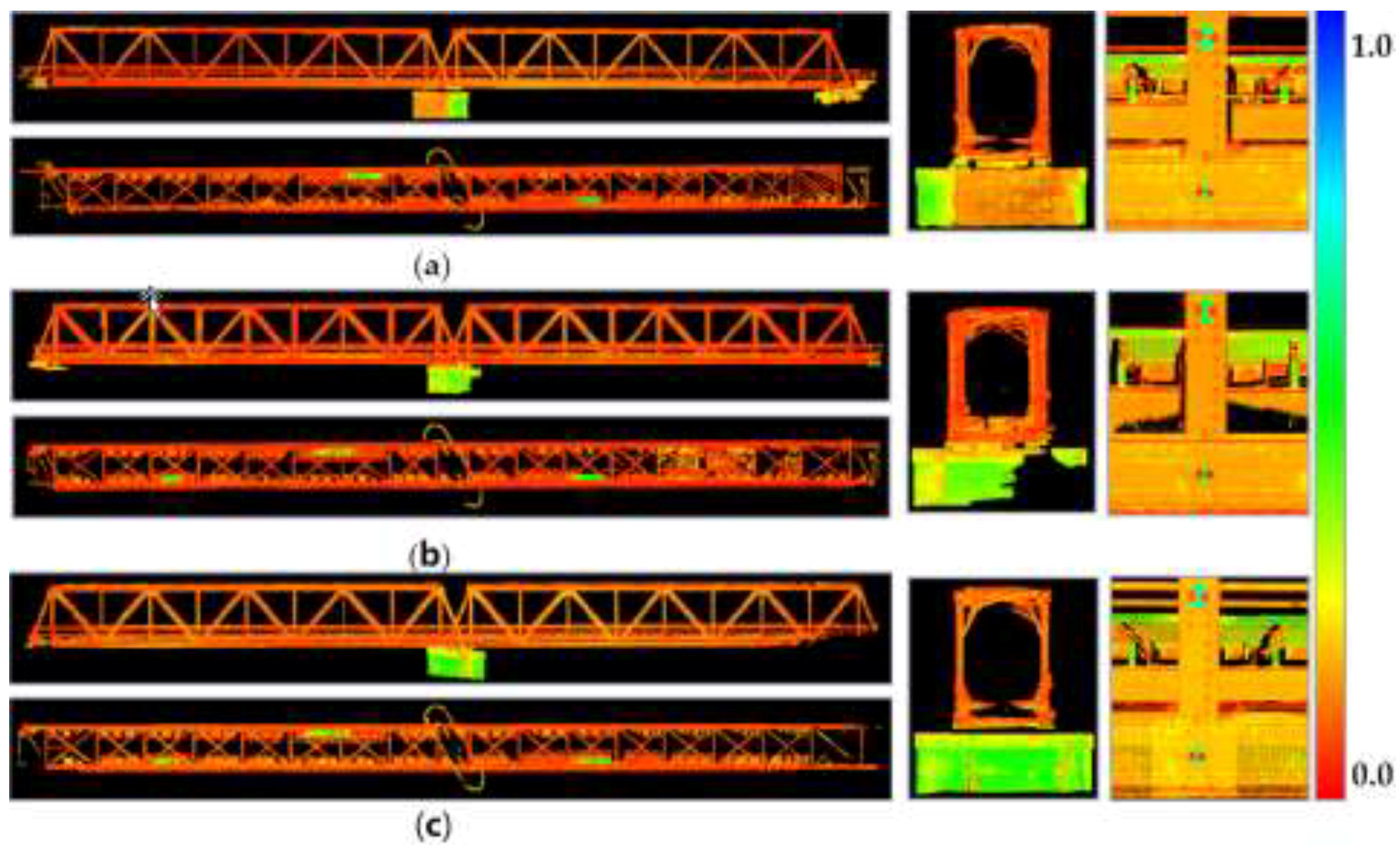
3.4. Case Study 3—Surfaces Meshes Analysis
4. Conclusions
Author Contributions
Funding
Conflicts of Interest
References
- Bień, J. Uszkodzenia i Diagnostyka Obiektów Mostowych [Damage to and Diagnostics of Bridges]; Wydawnictwa Komunikacji i Łączności: Warsaw, Poland, 2010. [Google Scholar]
- Taylor, W.M. Iron, engineering and architectural history in crisis: Following the case of the river Dee bridge disaster, 1847. Archit. Hist. 2013, 1, Art.23. [Google Scholar] [CrossRef]
- Klasztorny, M. Dynamika Mostów Belkowych Obciążonych Pociągami Szybkobieżnymi [Dynamics of Beam Bridges under High-Speed Train Load]; Wydawnictwa Naukowo-Techniczne: Warsaw, Poland, 2008. [Google Scholar]
- Kużawa, M.J.; Cruz, P.J.S.; Bień, J. Analysis and fatigue evaluation of Pinhao Bridge in Portugal. In Proceedings of the Mosty Stalowe: Projektowanie, Technologie Budowy, Badania, Utrzymanie, Wroclaw, Poland, 27–28 November 2008. [Google Scholar]
- Szadkowski, K. Mosty kolejowe—Przegląd inwestycji [Railway bridges—Review of investments]. In Proceedings of the Forum Budowy i Utrzymania Obiektów Inżynieryjnych Mosty 2015, Wieliczka, Poland, 24 June 2015. [Google Scholar]
- Duranton, S.; Audier, A.; Hazan, J.; Gauche, V. The 2015 European Railway Performance Index. Available online: https://www.bcg.com/publications/2015/rail-transportation-hubs-cost-efficiency-2015-european-railway-performance-index.aspx (accessed on 10 February 2019).
- Fraszczyk, A.; Lamb, T.; Marinov, M. Are railways really that bad? An evaluation of rail systems performance in Europe with a focus on passenger rail. Transp. Res. Part A Policy Pract. 2016, 94, 573–591. [Google Scholar] [CrossRef]
- Polish Government. Building Law Act of 7 July 1994; Polish Journal of Laws of 1994 No. 89, Item 414; Polish Government: Warsaw, Poland, 1994.
- Polish Government. Regulation of the Minister of Transport and Marine Economy of 10 September 1998 on Technical Conditions for Railway Structures and Their Location; Polish Journal of Laws of 1998 No. 151, Item 987; Polish Government: Warsaw, Poland, 1998.
- PKP PLK S.A. Id-16. (2005). Instrukcja Utrzymania Kolejowych Obiektów Inżynieryjnych [Maintenance Manual for Railway Civil Structures]; PKP PLK S.A.: Warsaw, Poland, 2005. [Google Scholar]
- PKP PLK S.A. Id-16. (2014). Instrukcja Utrzymania Kolejowych Obiektów Inżynieryjnych [Maintenance Manual for Railway Civil Structures]; PKP PLK S.A.: Warsaw, Poland, 2014. [Google Scholar]
- Standardy Techniczne. Szczegółowe Warunki Techniczne dla Modernizacji lub Budowy Linii Kolejowych do Prędkości Vmax ≤ 200 km/h (dla Taboru Konwencjonalnego)/250 km/h (dla Taboru z Wychylnym Pudłem) [Detailed Technical Requirements for Upgrading or Construction of Railway liNes to Vmax ≤ 200 km/h (for Standard Rolling Stock) or 250 km/h (for Tilting Rolling Stock)]; Volume I Track road; PKP PLK SA: Warsaw, Poland, 2009. [Google Scholar]
- The Polish Committee for Standardization. PN-S-10030:1985 Bridges–Loads; The Polish Committee for Standardization: Warsaw, Poland, 1985. [Google Scholar]
- The Polish Committee for Standardization. PN-S-10050:1989 Bridges–Steel Structures–Requirements and Tests; The Polish Committee for Standardization: Warsaw, Poland, 1989. [Google Scholar]
- The Polish Committee for Standardization. PN-S-10040:1999 Bridges. Concrete, Reinforced Concrete, and Prestressed Structures. Requirements and Tests; The Polish Committee for Standardization: Warsaw, Poland, 1999. [Google Scholar]
- Salamak, M.; Łaziński, P.; Pradelok, S.; Będkowski, P. Badania odbiorcze mostów kolejowych pod próbnym obciążeniem dynamicznym—Wymagania i praktyka [Acceptance tests for railway bridges under a dynamic test load—Requirements and practice]. In Proceedings of the Konferencja Naukowo-Techniczna INFRASZYN 2014, Zakopane, Poland, 9–11 April 2014. [Google Scholar]
- The Polish Committee for Standardization. PN-EN 1990:2004 Basis of Structural Design; The Polish Committee for Standardization: Warsaw, Poland, 2004. [Google Scholar]
- Hiremagalur, J.; Yen, K.; Akin, K.; Bui, T.; Lasky, T.; Ravani, B. Creating Standards and Specifications for the Use of Laser Scanning in Caltrans Projects; AHMCT Research Report, 2007, California AHMCT Program; University of California at Davis California Department of Transportation: Davis, CA, USA, 2007. [Google Scholar]
- Lichti, D.D.; Stewart, M.P.; Taskiri, M.; Snow, A.J. Benchmark tests on a three dimensional laser scanning system. Geomat. Res. Australas. 2002, 72, 1–23. [Google Scholar]
- Boehler, W.; Bordas, M.; Marbs, A. Investigating laser scanner accuracy. In Proceedings of the CIPA XIXth International Symposium, Antalya, Turkey, 30 September–4 October 2003. [Google Scholar]
- Cosarca, C.; Jocea, A.; Savu, A. Analysis of error sources in Terrestrial Laser Scanning. J. Geod. Cadaster 2009, 11, 115–124. [Google Scholar]
- Pesci, A.; Teza, G. Effects of surface irregularities on intensity data from laser scanning: An experimental approach. Ann. Geophys. 2008, 51, 839–848. [Google Scholar]
- Clark, J.; Robson, S. Accuracy of measurements made with CYRAX 2500 laser scanner against surfaces of known colour. Int. Arch. Photogramm. Remote Sens. Spat. Inf. Sci. 2004, XXXV, 1031–1037. [Google Scholar] [CrossRef]
- Mitka, B. Możliwości zastosowania naziemnych skanerów laserowych w procesie dokumentacji i modelowania obiektów zabytkowych [Using terrestrial laser scanning for archiving and modelling of historical objects]. Arch. Fotogram. Teledetekcji 2007, 17b, 525–534. [Google Scholar]
- Van Gosliga, R.; Lindenbergh, R.; Pfeifer, N. Deformation analysis of a bored tunnel by means of terrestrial laser scanning. Image Eng. Vis. Metrol. 2006, XXXVI, 167–172. [Google Scholar]
- Bitelli, G.; Dubbini, M.; Zanutta, A. Terrestrial laser scanning and digital photogrammetry techniques to monitor landslides bodies. Int. Arch. Photogramm. Remote Sens. Spat. Inf. Sci. 2004, 35, 246–251. [Google Scholar]
- Schäfer, T.; Weber, T.; Kyrinovic, P.; Zámecniková, M. Deformation measurement using terrestrial laser scanning at the hydropower station of Gabcikovo. In Proceedings of the INGEO 2004 and FIG Regional Central and Eastern European Conference on Engineering Surveying, Bratislava, Slovakia, 11–13 November 2004. [Google Scholar]
- Zogg, H.M.; Ingensand, H. Terrestrial laser scanning for deformation monitoring-load tests on the Felsenau Viaduct (ch). Int. Arch. Photogramm. Remote Sens. Inf. Sci. 2008, XXXVII, 555–562. [Google Scholar]
- Shen-En, C. Laser scanning technology for bridge monitoring. In Laser Scanner Technology; Rodriguez, J.A.M., Ed.; InTech: Vienna, Austria, 2012; ISBN 978-953-51-0280-9. [Google Scholar]
- Van Genechten, B.; Schueremans, L. Laserscanning for heritage documentation. Wiadomości Konserw. 2009, 26, 727–737. [Google Scholar]
- Monserrat, O.; Crosetto, M. Deformation measurement using terrestrial laser scanning data and least squares 3D surface matching. ISPRS J. Photogramm. Remote Sens. 2008, 63, 142–154. [Google Scholar] [CrossRef]
- Rosser, N.J.; Petley, D.N.; Lim, M.; Dunning, S.A.; Allison, R.J. Terrestrial laser scanning for monitoring the process of hard rock coastal cliff erosion. Q. J. Eng. Geol. Hydrogeol. 2005, 38, 363–375. [Google Scholar] [CrossRef]
- Alba, M.; Fregonese, L.; Prandi, F.; Scaioni, M.; Valgoi, P. Structural monitoring of a large dam by terrestrial laser scanning. Int. Arch. Photogramm. Remote Sens. Spat. Inf. Sci. 2006, 36, 6. [Google Scholar]
- Ioannidis, C.; Valani, A.; Georgopoulos, A.; Tsiligiris, E. 3D model generation for deformation analysis using laser scanning data of a cooling tower. In Proceedings of the 12th FIG Symposium, Baden, Austria, 22–24 May 2006. [Google Scholar]
- Lõhmus, H.; Ellmann, A.; Märdla, S.; Idnurm, S. Terrestrial laser scanning for the monitoring of bridge load tests—Two case studies. Surv. Rev. 2018, 50, 270–284. [Google Scholar] [CrossRef]
- Yilmaz, H.M.; Yakar, M.; Yildiz, F.; Karabork, H.; Kavurmaci, M.M.; Mutluoglu, O.; Goktepe, A. Monitoring of corrosion in fairy chimney by terrestrial laser scanning. J. Int. Environ. Appl. Sci. 2009, 4, 86–91. [Google Scholar]
- Erdélyi, J. Exploitation of TLS at deformation monitoring of bridge structure. In Proceedings of the INGEO 2011—5th International Conference on Engineering Surveying Brijuni, Brijuni, Croatia, 22–24 September 2011. [Google Scholar]
- Kašpar, M.; Pospišil, J.; Štroner, M.; Kŕemen, T.; Tejkal, M. Laser Scanning in Civil Engineering and Land Surveying; Czech s.r.o.: Hradce Králové, Czech Republic, 2004; ISBN 80-900860-7-1. [Google Scholar]
- Gawronek, P.; Kumisiński, W.; Kwinta, A.; Patykowski, G.; Zygmunt, M. Zastosowanie naziemnego skaningu laserowego w badaniu górniczych obiektów inżynierskich [The application of terrestrial laser scanning in the investigation of mining civil structures]. Bezpieczeństwo Pr. Ochr. Środowiska Górnictwie 2016, 2, 14–22. [Google Scholar]
- Lovas, T.; Barsi, A.; Detrekoi, A.; Dunai, L.; Csak, Z.; Polgar, A.; Berenyi, A.; Kibedy, Z.; Szocs, K. Terrestrial laserscanning in deformation measurements of structures. Int. Arch. Photogramm. Remote Sens. Spat. Inf. Sci. 2008, 37, 527–532. [Google Scholar]
- Nuttens, A.; De Wulf, L.; Bral, L.; De Wit, B.; Carlier, L.; De Ryck, M.; Stal, C.; Constales, D.; De Backer, H. High resolution terrestrial laser scanning for tunnel deformation measurements. In Proceedings of the FIG Congress, Sydney, Australia, 11–16 April 2010. [Google Scholar]
- Gawronek, P.; Makuch, M. TLS measurement during static load testing of a railway bridge. ISPRS Int. J. Geo Inf. 2019, 8, 44. [Google Scholar] [CrossRef]
- The Polish Committee for Standardization. PN-N-02211:2000 Surveying–Survey Displacement Determination–Basic Terms; The Polish Committee for Standardization: Warsaw, Poland, 2000. [Google Scholar]
- Gawronek, P. Methodology of Determining Stability of Bridges Using Terrestrial Laser Scanning. Ph.D. Thesis, Faculty of Environmental Engineering and Land Surveying, University of Agriculture in Krakow, Kraków, Poland, 2017. (In Polish). [Google Scholar]
- Girardeau-Montaut, D.; Roux, M.; Marc, R.; Thibault, G. Change detection on points cloud data acquired with a ground laser scanner. IAPRS SIS 2005, 36, 30–35. [Google Scholar]
- Lague, D.; Brodu, N.; Leroux, J. Accurate 3D comparison of complex topography with terrestrial laser scanner: Application to the Rangitikei Canyon (N-Z). ISPRS J. Photogramm. Remote Sens. 2013. [Google Scholar] [CrossRef]
- Mill, T.; Ellmann, A.; Kisa, M.; Idnurm, J.; Idnurm, S.; Horemuz, M.; Aavik, A. Geodetic monitoring of bridge deformations occurring during static load testing. Balt. J. Road Bridge Eng. 2015, 10, 17–27. [Google Scholar] [CrossRef] [Green Version]
- Toś, C.; Wolski, B.; Zielina, L. Zastosowanie tachimetru skanującego w praktyce geodezyjnej [The application of scanning total stations in surveying practice]. Environ. Czas. Technol. 2010, 17, 83–99. [Google Scholar]
- Quintero, M.S.; Genechten, B.; Bruyne, M.; Poelman, R.; Hankar, M.; Barnes, S.; Caner, H.; Craven, P.; Budei, L.; Heine, E.; et al. 3D RiskMapping. In Theory and Practice on Terrestrial Laser Scanning. Training Material Based on Practicial Applications. Prepared by the Learning Tools for Advanced Three-Dimensional Surveying in Risk Awareness Project; Universidad Politecnica de Valencia Editorial: València, Spain, 2008. [Google Scholar]
- Krysicki, W.; Bartos, J.; Dyczka, W.; Królikowska, K.; Wasilewski, M. Rachunek Prawdopodobieństwa i Statystyka Matematyczna w Zadaniach [Probability Calculus and Mathematical Statistics. Exercises]; Part II. Mathematical Statistics. Issue IV; Wydawnictwo Naukowe PWN: Warsaw, Poland, 1999. [Google Scholar]
- Plucińska, A.; Pluciński, E. Probabilistyka [Calculus of Probability]; Wydawnictwo Naukowo-Techniczne: Warsaw, Poland, 2000. [Google Scholar]
- Abellàn, A.; Jaboyedoff, M.; Oppikofer, T.; Vilaplana, J.M. Detection of millimetric deformation using a terrestrial laser scanner: Experiment and application to a rockfall event. Nat. Hazards Earth Syst. Sci. 2009, 9, 365–372. [Google Scholar] [CrossRef]
- Delaloye, D. Development of a New Methodology for Measuring Deformation in Tunnels and Shafts with Terrestrial Laser Scanning (LIDAR) Using Elliptical Fitting Algorithms. Master’s Thesis, Queen’s University, Kingston, ON, Canada, 2012. [Google Scholar]
- Oliveira, A.; Oliveira, J.F.; Pereira, J.M.; De Araújo, B.R.; Boavida, J. 3D modelling of laser scanned and photogrammetric data for digital documentation: The Mosteiro da Batalha case study. J. Real Time Image Process. 2014, 9, 673–688. [Google Scholar] [CrossRef]


 |  |  |  |  |
|---|---|---|---|---|
| PN-89/S-10050 | PN-99/S-10040 | Id-16 Instructions (2005) | Id-16 Instructions (2014) | PKP Standards (2009) |
| Static Load Test | ||||
| L * > 21 m | Every bridge | Every bridge | Not applicable | Every bridge |
| Dynamic Load Test | ||||
| L > 21 m | L = approx. 15 m | Steel: L > 21 m Concrete: L > 10 m | Not applicable | L > 21 m |
| Goals | ||
|---|---|---|
| I | Precise leveling of bridge spans | The vertical displacements of protrusions of the main girders of the bridge |
| Reference measurements for TLS results | ||
| II | Reflectorless precision tacheometry of controlled points | The displacements of controlled point network |
| Reference measurements for TLS results | ||
| III | Terrestrial laser scanning | The displacements of the bridge determined using:
|
| Aims | |
|---|---|
| Precise leveling | Periodic precise leveling of the control network |
| Precise leveling of white sphere targets | |
| Periodic precise leveling of the main girders of the bridge | |
| Precise tacheometry, reflection-based measurement | Periodic measurement of the control network |
| Precise tacheometry, reflectorless measurement | Periodic measurement of the controlled point network |
| Terrestrial laser scanning | Periodic measurement of the bridge |
| Instrument | Technical Parameters |
|---|---|
| Leica NA3003 | Measuring distance: 1.3–100 m |
| Precision of distance measurement: ± (3 mm + 5 pmm) | |
| Accuracy per 1 km of double leveling: 0.4 mm (invar staff), 1.2 mm (standard staff) | |
| Trimble VX | Maximum measuring distance: 250 m |
| Precision of distance measurement: ± (1 mm + 2 pmm) | |
| Angular accuracy 1″ | |
| Z+F Imager 5010 | Maximum measuring distance: 187 m |
| Beam divergence < mrad (full angle) | |
| Beam diameter approx. 3.5 mm per 1 m | |
| More than 1 million pixel/sec maximum measurement rate |
| CASE STUDY 1 Controlled Point Network | CASE STUDY 2 Point Clouds | CASE STUDY 3 Surface Mesh | |
|---|---|---|---|
| Methodology of determining displacements by TLS | periodic comparison of changes in the spatial position of elements of the controlled point network | periodic comparison of point clouds by generating differential point cloud models of the main bridge girders, analysis of vertical displacements | periodic comparison of surface models by generating differential surface models of the main bridge girders, analysis of vertical displacements |
| Reference measurements | displacements of elements of the controlled point network, determined by reflectorless tacheometry | the vertical displacements of nodes of the main girders, determined by precise leveling | the vertical displacements of the nodes of the main girders, determined by precise leveling |
| - | point clouds of the object | - | |
| Sets of input TLS data | registered point clouds of the object, with the georeferenced control network | registered point clouds of the object, with the georeferenced control network | registered point clouds of the object, with the georeferenced control network |
| - | second set of input data with the use of filtration algorithms | second set of input data with the use of filtration algorithms |
| Stage 1 | Tie Points | Georeference Data | 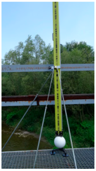 | |
| 1 | HDS (High-Definition Surveying) targets | 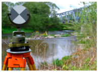 | (X, Y) of points of the control network | |
| 2 | white sphere targets 2 |  | (X, Y) of sphere targets from the results of the first stage (H) of the centers of the sphere targets from precise leveling | |
| REGISTRATION | First Series | Second Series | Third Series | |
| MAE [m] | 0.001 | 0.001 | 0.001 | |
| RMS [m] | 0.002 | 0.001 | 0.002 | |
| FILTRATION | Number of Elements in Point Clouds | |||
| Filtration Stage | Filtration Algorithm | First Series | Second Series | Third Series |
| - | Periodic point cloud | 48,531,393 | 53,926,203 | 24,984,892 |
| 1 | SOR filter | 45,665,543 | 49,787,683 | 24,368,852 |
| 2 | Noise filter | 43,137,503 | 47,036,862 | 22,828,872 |
| 3 | Bilateral filter | 43,053,399 | 47,020,857 | 22,828,515 |
| Percentage of the reduction of the elements of point clouds [%] | 11 | 13 | 9 | |
| (a) Epochs 1–2 | ||||
| Displacement | Significance Level α | Cluster Analysis | Statistic Value λ (D = sup| F1(TLS) − F2(TACH)|) | Resultant Hypothesis |
| along the OX axis | α = 0.01 | 0.001 m | λ = 1.25 < λα = 1.63 | H0 |
| along the OY axis | λ = 1.25 < λα = 1.63 | H0 | ||
| vertical | λ = 0.97 < λα = 1.63 | H0 | ||
| (b) Epochs 1–3 | ||||
| Displacement | Significance Level α | Cluster Analysis | Statistic Value λ (D = sup| F1(TLS) − F2(TACH)|) | Resultant Hypothesis |
| along the OX axis | α = 0.01 | 0.001 m | λ = 1.07 < λα = 1.63 | H0 |
| along the OY axis | λ = 0.80 < λα = 1.63 | H0 | ||
| vertical | λ = 0.80 < λα = 1.63 | H0 | ||
| (a) First Sets of Data | ||||
| Epoch | Significance Level α | Cluster Analysis | Statistic Value λ (D = sup| F1(TLS) − F2(LEV)|) | Resultant Hypothesis |
| 1–2 | α = 0.01 | 0.001 m | λ = 1.66 > λα = 1.63 | H1 |
| 1–3 | λ = 2.04 > λα = 1.63 | H1 | ||
| (b) Second Sets of Data | ||||
| Epoch | Significance Level α | Cluster Analysis | Statistic Value λ (D = sup| F1(TLS) − F2(LEV)|) | Resultant Hypothesis |
| 1–2 | α = 0.01 | 0.001 m | λ = 0.92 < λα = 1.63 | H0 |
| 1–3 | λ = 0.82 < λα = 1.63 | H0 | ||
| (c) Third Sets of Data | ||||
| Epoch | Significance Level α | Cluster Analysis | Statistic Value λ (D = sup| F1(TLS) − F2(LEV)|) | Resultant Hypothesis |
| 1–2 | α = 0.01 | 0.001 m | λ = 0.62 < λα = 1.63 | H0 |
| 1–3 | λ = 0.63 < λα = 1.63 | H0 | ||
| (a) Second sets of data | ||||
| Epoch | Significance Level α | Cluster Analysis | Statistic Value λ (D = sup| F1(TLS) − F2(LEV)|) | Resultant Hypothesis |
| 1–2 | α = 0.01 | 0.001 m | λ = 0.56 < λα = 1.63 | H0 |
| 1–3 | λ = 1.45 < λα = 1.63 | H0 | ||
| (b) Third sets of data | ||||
| Epoch | Significance Level α | Cluster Analysis | Statistic Value Λ (D = sup| F1(TLS) − F2(LEV)|) | Resultant Hypothesis |
| 1–2 | α = 0.01 | 0.001 m | λ = 0.46 < λα = 1.63 | H0 |
| 1–3 | λ = 0.82 < λα = 1.63 | H0 | ||
| (a) Case Study 2 | First Set of Data | Second Set of Data | Third Set of Data |
| * | ±2.4 | ±2.4 | ±2.4 |
| * | ±2.3 | ±1.2 | ±1.5 |
| * | ±1.9 | ±0.9 | ±1.0 |
| * | ±4.0 | ±2.5 | ±3.2 |
| * | 0.8 | 0.5 | -0.2 |
| (b) Case Study 3 | Second Set of Data | Third Set of Data | |
| * | ±2.4 | ±2.4 | |
| * | ±4.3 | ±2.2 | |
| * | ±2.5 | ±1.3 | |
| * | ±12.9 | ±4.5 | |
| * | 1.7 | 0.1 |
© 2019 by the authors. Licensee MDPI, Basel, Switzerland. This article is an open access article distributed under the terms and conditions of the Creative Commons Attribution (CC BY) license (http://creativecommons.org/licenses/by/4.0/).
Share and Cite
Gawronek, P.; Makuch, M.; Mitka, B.; Gargula, T. Measurements of the Vertical Displacements of a Railway Bridge Using TLS Technology in the Context of the Upgrade of the Polish Railway Transport. Sensors 2019, 19, 4275. https://doi.org/10.3390/s19194275
Gawronek P, Makuch M, Mitka B, Gargula T. Measurements of the Vertical Displacements of a Railway Bridge Using TLS Technology in the Context of the Upgrade of the Polish Railway Transport. Sensors. 2019; 19(19):4275. https://doi.org/10.3390/s19194275
Chicago/Turabian StyleGawronek, Pelagia, Maria Makuch, Bartosz Mitka, and Tadeusz Gargula. 2019. "Measurements of the Vertical Displacements of a Railway Bridge Using TLS Technology in the Context of the Upgrade of the Polish Railway Transport" Sensors 19, no. 19: 4275. https://doi.org/10.3390/s19194275