Fast Method for Liquid Crystal Cell Spatial Variations Estimation Based on Modeling the Spectral Transmission

 ,
,  and
and 
Abstract
:1. Introduction
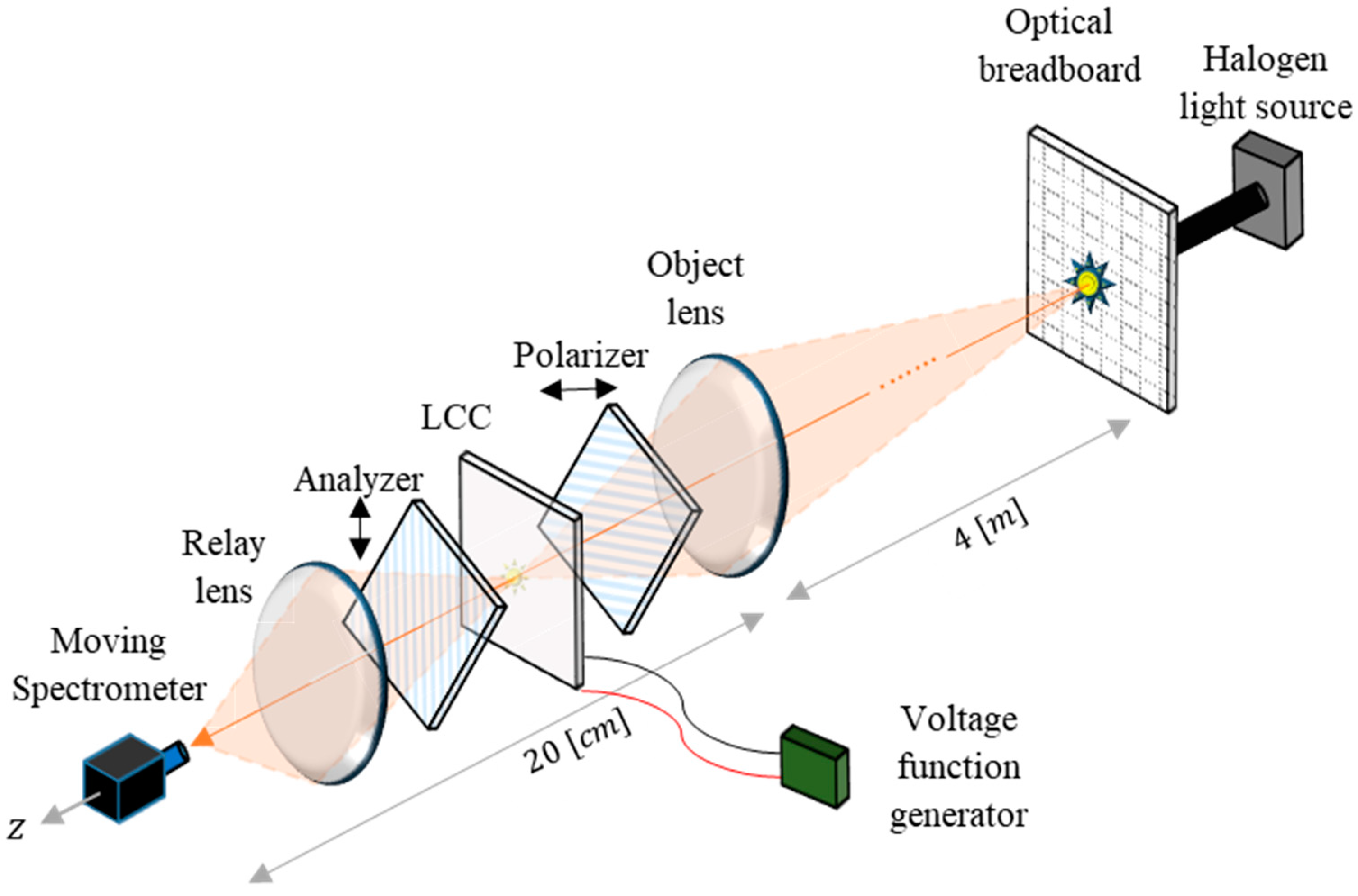
2. Optical Calibration Setup
3. Spectral Transmission Parametric Modeling and Spatial Estimation Method
3.1. Spectral Transmission Parametric Modeling
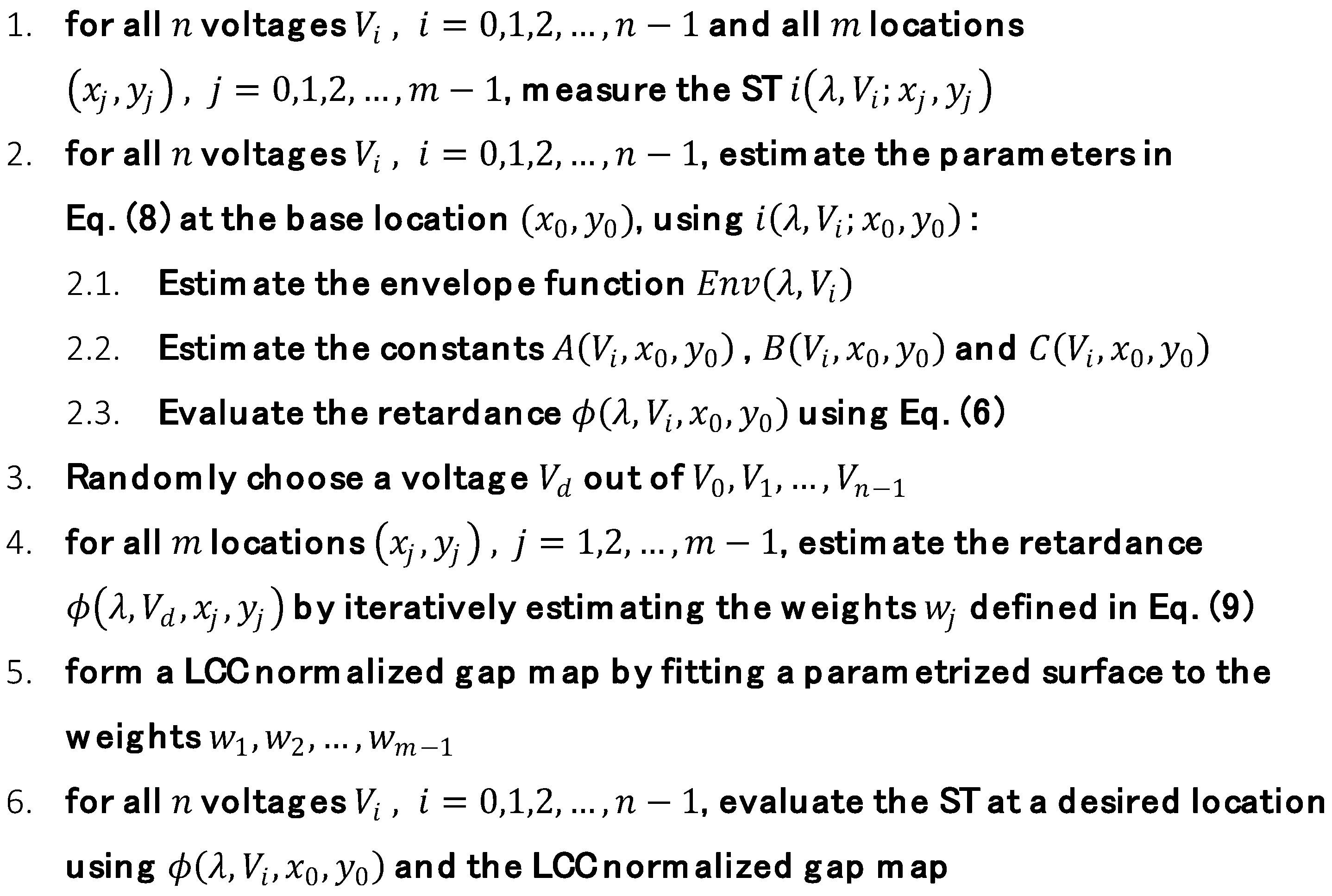
3.2. Spatial Estimation
4. Results
4.1. Simulation
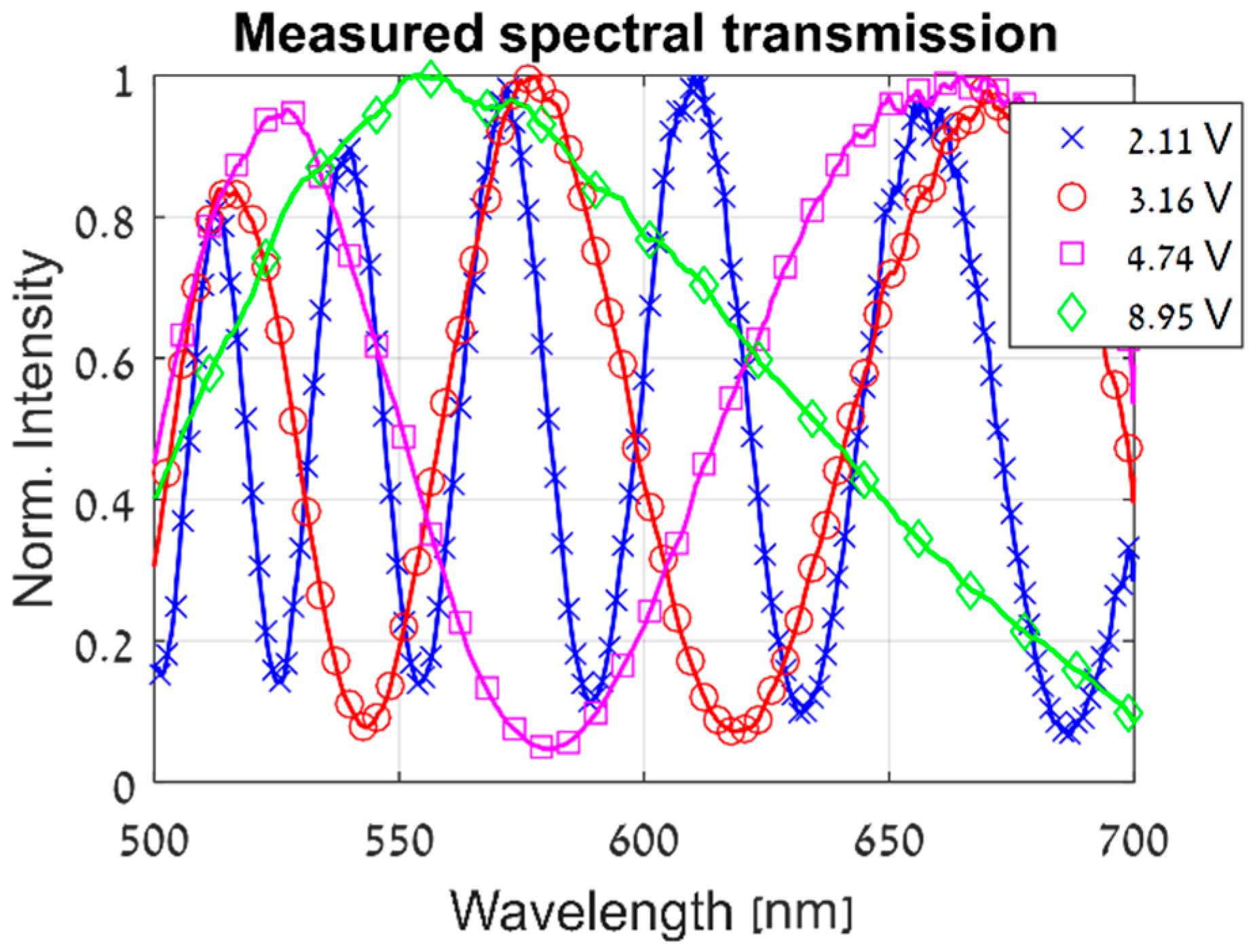
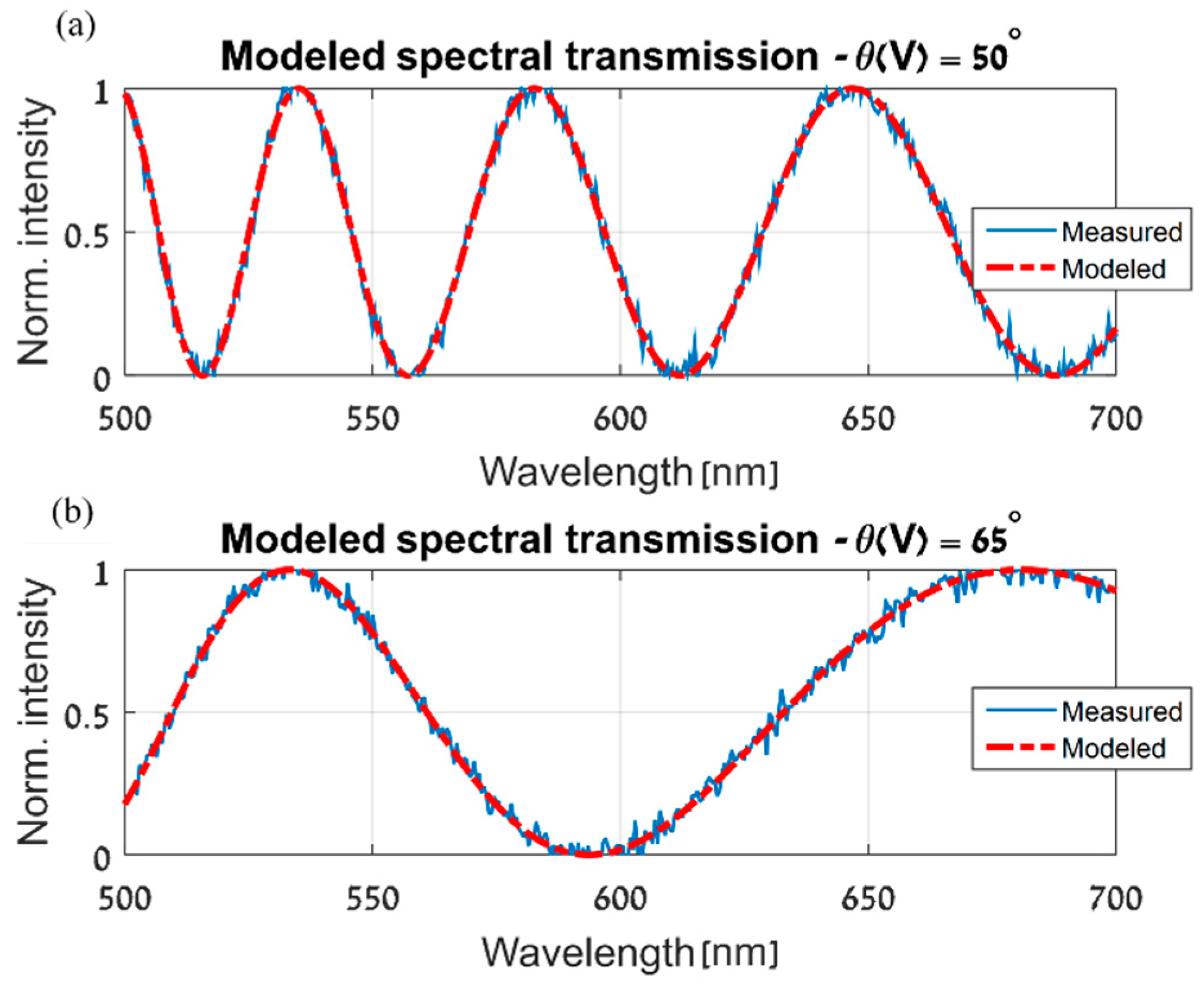
4.2. Experiment
5. Conclusions
Author Contributions
Funding
Conflicts of Interest
References
- Abdulhalim, I. Non-Display Bio-Optic Applications of Liquid Crystals. Liq. Cryst. Today 2011, 20, 44–60. [Google Scholar] [CrossRef]
- Abdulhalim, I. Liquid Crystal Active Nanophotonics and Plasmonics: From Science to Devices. J. Nanophotonics 2012, 6, 061001. [Google Scholar] [CrossRef]
- Javidi, B.; Shen, X.; Markman, A.S.; Latorre-Carmona, P.; Martinez-Uso, A.; Sotoca, J.M.; Pla, F.; Martinez-Corral, M.; Saavedra, G.; Huang, Y. Multidimensional Optical Sensing and Imaging System (MOSIS): From Macroscales to Microscales. Proc. IEEE 2017, 105, 850–875. [Google Scholar] [CrossRef]
- Kurihara, J.; Takahashi, Y.; Sakamoto, Y.; Kuwahara, T.; Yoshida, K. HPT: A High Spatial Resolution Multispectral Sensor for Microsatellite Remote Sensing. Sensors 2018, 18, 619. [Google Scholar] [CrossRef] [PubMed]
- Gebhart, S.C.; Thompson, R.C.; Mahadevan-Jansen, A. Liquid-Crystal Tunable Filter Spectral Imaging for Brain Tumor Demarcation. Appl. Opt. 2007, 46, 1896–1910. [Google Scholar] [CrossRef]
- Imai, F.H.; Rosen, M.R.; Berns, R.S. Multi-Spectral Imaging of a Van Gogh’s Self-Portrait at the National Gallery of Art Washington DC. In Proceedings of the PICS 2001: Image Processing, Image Quality, Image Capture, Systems Conference, Montréal, QC, Canada, 22–25April 2001; pp. 185–189. [Google Scholar]
- Abuleil, M.J.; Abdulhalim, I. Tunable Achromatic Liquid Crystal Waveplates. Opt. Lett. 2014, 39, 5487–5490. [Google Scholar] [CrossRef] [PubMed]
- Abuleil, M.J.; Abdulhalim, I. Broadband Ellipso-Polarimetric Camera Utilizing Tunable Liquid Crystal Achromatic Waveplate with Improved Field of View. Opt. Express 2019, 27, 12011–12024. [Google Scholar] [CrossRef]
- Vargas, J.; Uribe-Patarroyo, N.; Quiroga, J.A.; Alvarez-Herrero, A.; Belenguer, T. Optical Inspection of Liquid Crystal Variable Retarder Inhomogeneities. Appl. Opt. 2010, 49, 568–574. [Google Scholar] [CrossRef]
- Vargas, A.; Donoso, R.; Ramírez, M.; Carrión, J.; del Mar Sánchez-López, M.; Moreno, I. Liquid Crystal Retarder Spectral Retardance Characterization Based on a Cauchy Dispersion Relation and a Voltage Transfer Function. Opt. Rev. 2013, 20, 378–384. [Google Scholar] [CrossRef]
- Bennett, T.; Proctor, M.; Forster, J.; Perivolari, E.; Podoliak, N.; Sugden, M.; Kirke, R.; Regrettier, T.; Heiser, T.; Kaczmarek, M.; et al. Wide area mapping of liquid crystal devices with passive and active command layers. Appl. Opt. 2017, 56, 9050–9056. [Google Scholar] [CrossRef]
- Tang, S.; Kwok, H. Transmissive Liquid Crystal Cell Parameters Measurement by Spectroscopic Ellipsometry. J. Appl. Phys. 2001, 89, 80–85. [Google Scholar] [CrossRef]
- Lee, S.H.; Park, W.S.; Lee, G.; Han, K.; Yoon, T.; Kim, J.C. Low-Cell-Gap Measurement by Rotation of a Wave Retarder. Jpn. J. Appl. Phys. 2002, 41, 379. [Google Scholar] [CrossRef]
- August, I.; Oiknine, Y.; AbuLeil, M.; Abdulhalim, I.; Stern, A. Miniature Compressive Ultra-spectral Imaging System Utilizing a Single Liquid Crystal Phase Retarder. Sci. Rep. 2016, 6, 23524. [Google Scholar] [CrossRef] [PubMed]
- Oiknine, Y.; August, I.; Stern, A. Along-track scanning using a liquid crystal compressive hyperspectral imager. Opt. Express 2016, 24, 8446–8457. [Google Scholar] [CrossRef] [PubMed]
- Gedalin, D.; Oiknine, Y.; August, I.; Blumberg, D.G.; Rotman, S.R.; Stern, A. Performance of target detection algorithm in compressive sensing miniature ultraspectral imaging compressed sensing system. Opt. Eng. 2017, 56, 041312. [Google Scholar] [CrossRef]
- Oiknine, Y.; August, I.; Farber, V.; Gedalin, D.; Stern, A. Compressive Sensing Hyperspectral Imaging by Spectral Multiplexing with Liquid Crystal. J. Imaging 2019, 5, 3. [Google Scholar] [CrossRef]
- Stern, A. Optical Compressive Imaging; CRC Press: Boca Raton, FL, USA, 2016. [Google Scholar]
- Yariv, A.; Yeh, P. Optical Waves in Crystals; Wiley: New York, NY, USA, 1984. [Google Scholar]
- Lu, K.; Saleh, B.E. Theory and Design of the Liquid Crystal TV as an Optical Spatial Phase Modulator. Opt. Eng. 1990, 29, 240–247. [Google Scholar] [CrossRef]
- Saleh, B.E.; Teich, M.C. Fundamentals of Photonics; John Wiley&Sons: Hoboken, NJ, USA, 2019. [Google Scholar]
- Hecht, E. Optics, 4th ed.; Addison Wesley Longman: Boston, MA, USA, 1998. [Google Scholar]
- Jenkins, F.A.; White, H.E. Fundamental of Optics, 4th ed.; McGraw-Hill Education: New York, NY, USA, 2001. [Google Scholar]
- Li, J.; Wen, C.; Gauza, S.; Lu, R.; Wu, S. Refractive Indices of Liquid Crystals for Display Applications. J. Disp. Technol. 2005, 1, 51. [Google Scholar] [CrossRef]
- Abuleil, M.J.; Abdulhalim, I. Birefringence Measurement using Rotating Analyzer Approach and Quadrature Cross Points. Appl. Opt. 2014, 53, 2097–2104. [Google Scholar] [CrossRef]
- Wahle, M.; Kitzerow, H. Liquid Crystal Assisted Optical Fibres. Opt. Express 2014, 22, 262–273. [Google Scholar] [CrossRef]
- Oiknine, Y.; August, I.; Blumberg, D.G.; Stern, A. NIR hyperspectral compressive imager based on a modified Fabry–Perot resonator. J. Opt. 2018, 20, 044011. [Google Scholar] [CrossRef]
- Oiknine, Y.; August, I.; Stern, A. Multi-aperture snapshot compressive hyperspectral camera. Opt. Lett. 2018, 43, 5042–5045. [Google Scholar] [CrossRef] [PubMed]


© 2019 by the authors. Licensee MDPI, Basel, Switzerland. This article is an open access article distributed under the terms and conditions of the Creative Commons Attribution (CC BY) license (http://creativecommons.org/licenses/by/4.0/).
Share and Cite
Shmilovich, S.; Revah, L.; Oiknine, Y.; August, I.; Abdulhalim, I.; Stern, A. Fast Method for Liquid Crystal Cell Spatial Variations Estimation Based on Modeling the Spectral Transmission. Sensors 2019, 19, 3874. https://doi.org/10.3390/s19183874
Shmilovich S, Revah L, Oiknine Y, August I, Abdulhalim I, Stern A. Fast Method for Liquid Crystal Cell Spatial Variations Estimation Based on Modeling the Spectral Transmission. Sensors. 2019; 19(18):3874. https://doi.org/10.3390/s19183874
Chicago/Turabian StyleShmilovich, Shauli, Liat Revah, Yaniv Oiknine, Isaac August, Ibrahim Abdulhalim, and Adrian Stern. 2019. "Fast Method for Liquid Crystal Cell Spatial Variations Estimation Based on Modeling the Spectral Transmission" Sensors 19, no. 18: 3874. https://doi.org/10.3390/s19183874