Automatic Extraction of Water and Shadow from SAR Images Based on a Multi-Resolution Dense Encoder and Decoder Network
by
 , ,
, ,
Peng Zhang
1,2, 
Lifu Chen
1,2,3,*,
Zhenhong Li
3,4 ,
,
Jin Xing
3,
Xuemin Xing
2,5 and
Zhihui Yuan
1,2 1
School of Electrical and Information Engineering, Changsha University of Science & Technology, Changsha 410114, China
2
Laboratory of Radar Remote Sensing Applications, Changsha University of Science & Technology, Changsha 410014, China
3
School of Engineering, Newcastle University, Newcastle upon Tyne NE1 7RU, UK
4
College of Geological Engineering and Geomatics, Chang’an University, Xi’an 710054, China
5
School of Traffic & Transportation Engineering, Changsha University of Science & Technology, Changsha 410114, China
*
Author to whom correspondence should be addressed.
Sensors 2019, 19(16), 3576; https://doi.org/10.3390/s19163576
Submission received: 7 July 2019
/
Revised: 10 August 2019
/
Accepted: 12 August 2019
/
Published: 16 August 2019
(This article belongs to the Section Remote Sensors)
Abstract
:The water and shadow areas in SAR images contain rich information for various applications, which cannot be extracted automatically and precisely at present. To handle this problem, a new framework called Multi-Resolution Dense Encoder and Decoder (MRDED) network is proposed, which integrates Convolutional Neural Network (CNN), Residual Network (ResNet), Dense Convolutional Network (DenseNet), Global Convolutional Network (GCN), and Convolutional Long Short-Term Memory (ConvLSTM). MRDED contains three parts: the Gray Level Gradient Co-occurrence Matrix (GLGCM), the Encoder network, and the Decoder network. GLGCM is used to extract low-level features, which are further processed by the Encoder. The Encoder network employs ResNet to extract features at different resolutions. There are two components of the Decoder network, namely, the Multi-level Features Extraction and Fusion (MFEF) and Score maps Fusion (SF). We implement two versions of MFEF, named MFEF1 and MFEF2, which generate separate score maps. The difference between them lies in that the Chained Residual Pooling (CRP) module is utilized in MFEF2, while ConvLSTM is adopted in MFEF1 to form the Improved Chained Residual Pooling (ICRP) module as the replacement. The two separate score maps generated by MFEF1 and MFEF2 are fused with different weights to produce the fused score map, which is further handled by the Softmax function to generate the final extraction results for water and shadow areas. To evaluate the proposed framework, MRDED is trained and tested with large SAR images. To further assess the classification performance, a total of eight different classification frameworks are compared with our proposed framework. MRDED outperformed by reaching 80.12% in Pixel Accuracy (PA) and 73.88% in Intersection of Union (IoU) for water, 88% in PA and 77.11% in IoU for shadow, and 95.16% in PA and 90.49% in IoU for background classification, respectively.
1. Introduction
Synthetic Aperture Radar (SAR) is an active imaging radar featuring the ability of all-day and all-weather observation. It has been broadly applied in many fields, such as military, agriculture, geo-hazards, and marine sciences [1]. SAR image classification, which identifies different types of land use and land cover, plays a pivotal role in the process of SAR image analysis. With the rapid development of remote sensing technology, the resolution of SAR images is continuously increasing; and the volume of data is getting bigger and bigger. Traditional SAR data analysis heavily relies on manually crafted features, which usually turns out to be an onerous task with huge volume of data. Therefore, it is urgent to investigate automatic procedures for SAR data processing and analysis.
In side-looking SAR or interferometric SAR (InSAR) intensity images, there are shadow areas caused by tall buildings, trees, and mountains. They are visualized as dark areas since no signal has been backscattered to the radar. In addition, many water areas on the surface of the Earth also display as very low intensity areas or nearly dark areas, since the reflection of water bodies is very similar to that of mirrors. The extraction of water and shadow areas needs to be addressed in many fields, such as flooding water evaluation [2], surface water detection [3], and building change detection [4]. Furthermore, water and shadow areas in SAR and InSAR intensity images are usually noisy, which hinder related applications, such as road extraction [5], InSAR phase filtering [6], phase unwrapping [7], Digital Elevation Model generation [8], and time-series analysis [9]. Therefore, accurate extraction of water and shadow areas, which is quite challenging to perform automatically at present with high accuracy. plays a pivotal role in SAR or InSAR image analysis. Meanwhile, deep learning has developed rapidly in recent years [10], which has been used in classification for remote sensing images in numerous projects and achieved promising performance [11,12,13]. Therefore, it is appealing to explore deep learning for automatic water and shadow extraction.
To accomplish this goal, a novel framework named Multi-Resolution Dense Encoder and Decoder (MRDED) has been proposed in this paper. There are three parts of MRDED: the Gray Level Gradient Co-occurrence Matrix (GLGCM), the Encoder network, and the Decoder network. First, the GLGCM is chosen as the low-level feature extraction approach because of its superior performance in extracting texture features from SAR images. Second, Residual Network (ResNet) is used as the Encoder to extract intermediate and high-level features of the targets. At last, the Decoder is designed to fuse the features extracted by the Encoder and further generate essential features for the final extraction of water and shadow. The contributions of this paper may be summarized as follows:
- (1)
- As far as we know, MRDED is the first deep neural network specifically designed for automatic extraction of water and shadow from SAR images. To tackle the noisy information, we integrate several well-established deep neural networks, such as Resnet, Dense Connection Network (DenseNet), and Global Convolutional Network (GCN). The enhanced accuracy in our experiment has indicated the success of our integration.
- (2)
- The integration of Resnet, DenseNet, and multi-resolution network has enabled the design of deeper neural network for SAR image analysis. This approach has transformed more layers of neural network into better feature representation at various resolutions.
- (3)
- To improve the performance of the Decoder, a high-level feature fusion approach has been invented. We have developed two implementations of the Multi-level Features Extraction and Fusion (MFEF) network, named MFEF1 and MFEF2, to generate separate score map. Then, these two score maps are fused with different weights to generate the final score map for water and shadow extraction. Our experiment has proved this kind of high-level feature fusion is effective for water and shadow extraction.
The rest of the paper is arranged as follows: Section 2 gives the background of the paper, which presents the-state-of-the-art of water and shadow extraction in SAR image analysis. Section 3 describes MRDED in detail, especially the building of MFEF1and MFEF2 in the Decoder network. The experiment is depicted in Section 4, and the classification results of water and shadow are compared with several existing frameworks. We discuss how to further improve the performance of MRDED in Section 5. Finally, we conclude the paper in Section 6.
2. Background
SAR image classification has been very critical for SAR image understanding, and its fast development has attracted considerable interests. Ranjani and Thiruvengadam [14] proposed a classification method based on the multi-level ratio of exponentially weighted means, to compute the optimal threshold of classification. However, this thresholding approach still required manual tuning, which was very challenging to set if the pixel values of different classes were close. Hou et al. [15] proposed a Markov Random Field (MRF) method to perform SAR classification, which combined contextual information and simulated annealing algorithm. However, its performance was largely affected by noise.
Classification has been an important component for water and shadow extraction from SAR images. Hong et al. [16] proposed a thresholding method to perform water extraction using SAR images and DEM, and they found that the extraction accuracy was greatly improved compared with experiments only using SAR images. Martinis et al. [17] evaluated four water extraction methods used at the German Aerospace Center, namely Water Mask Processor, Rapid Mapping of Flooding, TSX Flood Service, and TanDEM-X Water Indication Mask processor. These four methods achieved satisfactory water extraction results, with the accuracies higher than 90%. However, they were not completely automatic and some of them required auxiliary information (e.g., DEM datasets). Xie et al. [18] proposed a supervised water extraction method for urban area studies, which has combined both shape and polarimetric features from SAR images.
There has been limited progress in shadow extraction and existing works have largely depended on feature extraction approaches. Cellier et al. [19] studied the shadow extraction using the mean shift algorithm for building reconstruction, by fusing the amplitude and coherence of SAR images. The results indicated the extraction accuracy of shadows was significantly improved by fusion. Tison et al. [20] proposed a method by minimizing an energy function for InSAR images to identify shadow areas, which achieved good performance for isolated or high buildings. However, this shadow extraction was problematic when the building was low, or the noise of the interferometric phase was high. Jahangir et al. [21] paid special attention to shadows from different overlapping objects, which were tackled using Support Vector Machine (SVM) classification with multiple perspective SAR images. Papson and Narayanan [22] adopted Expectation Maximization to perform shadow extraction and used a Hidden Markov Model to improve the boundary identification of the shadow areas from SAR images, which could achieve 75% accuracy.
Deep learning has brought great advancements in the classification of optical images, which has been extended to SAR images classification. Long et al. [23] replaced the traditional classification method by a fully convolutional network (FCN) to perform optical image classification. The employment of FCN has been a solid contribution, but the accuracy was limited, and the details of extraction (e.g., the boundary of water bodies) were poor. Chen et al. [24] and Zheng et al. [25] improved the classification accuracy by using Conditional Random Fields (CRFs), respectively. Cheng et al. [26] exploited atrous convolution to generate high-resolution feature maps, which could reduce the loss of details during the down-sampling process of the deep learning. Lin et al. [27] and Peng et al. [28] investigated codec network to achieve high classification accuracy. Chen et al. [29] proposed an all-convolutional network without using fully connected layers, which obtained an accuracy of 99% in ten-type targets of MSTAR dataset. Huang et al. [30] presented a transfer learning method by designing an assembled CNN structure to perform classification from SAR images with limited labels, which achieved better classification accuracy. Lin et al. [31] proposed the convolutional highway unit to perform classification from SAR image, which could bring the accuracy of 99% in MSTAR dataset; but the accuracy would drop to 94.7% with reduced training data. Geng et al. [32] proposed the pre-processing method to extract preliminary and intermediate features, then automatic encoder was adopted to perform SAR image classification. To reduce the influence of speckle noise, the post-processing method has been frequently explored. Zhang et al. [33] investigated a dense Depthwise separable convolution network to perform water classification, which achieved high accuracy, but only tested with small-scale images.
Although deep learning has been proved to be a promising technique for classification, there are still several limitations to be addressed before it can be used for automatic extraction of water and shadow from SAR images. First, SAR images are very different from optical images, in which speckle noise presents an additional challenge for classification. Second, the existing networks for classification need to be tailored for enhanced context integration and features extraction for water and shadow. Third, the similarity between water and shadow often leads to considerable misclassifications using convolutional neural networks. Therefore, a novel deep learning framework, called MRDED, has been proposed in this paper specifically for water and shadow extraction with high accuracy from SAR images.
3. Datasets Description
The datasets used in the paper are millimeter InSAR datasets acquired in Xi’an (China) in 2013, including nine large-scale SAR images with dimensions of 10240 × 13050. An example of the large-scale SAR images and the corresponding ground truth are shown in Figure 1, where the capital characters ‘S’, ‘W’, and ‘B’ denote ‘Shadow’, ‘Water’, and ‘Background’, respectively. In the experiment, only SAR images are used, and the coherence map and InSAR phase are not included. First, we use the ‘Image Labeler’ in the MatLab software to mark the three types of targets, namely, water, shadow, and background. All the shadow and water labels are checked carefully by several SAR/InSAR experts. Then, the nine-labeled large-scale images are decomposed into numerous 720 × 720 tiles, except the area selected for testing in Section 5.1. There are 1288 image tiles in total, and the ratio of training samples and validation samples is set to 4:1.
4. Methodology
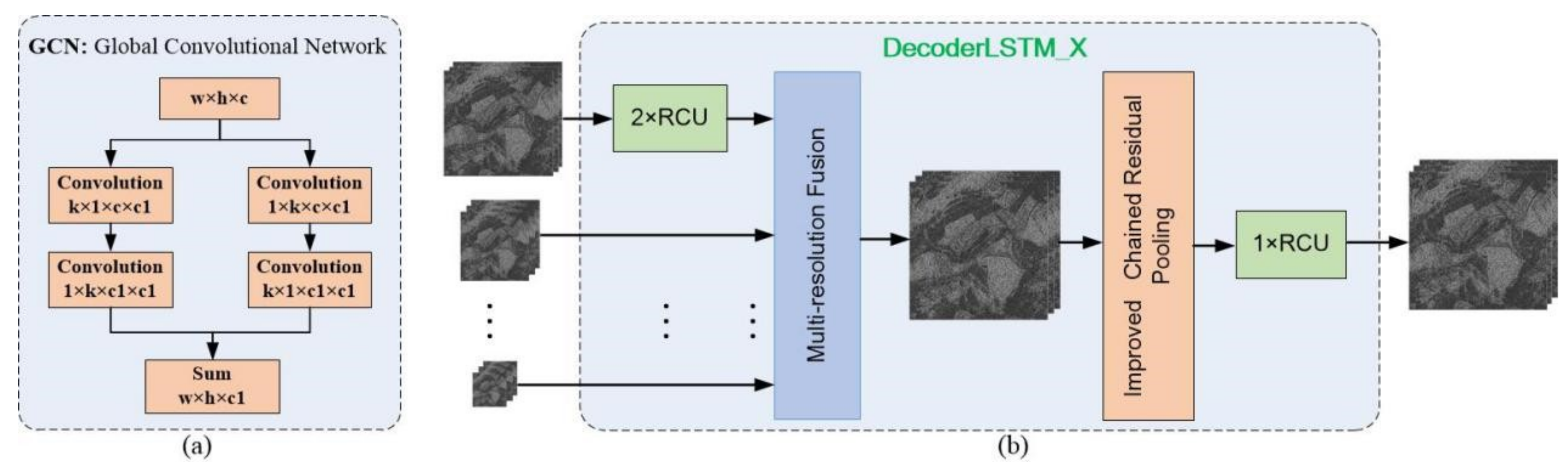
The proposed Multi-Resolution Dense Encoder and Decoder (MRDED) network integrates Convolutional Neural Network (CNN) [34], Dense Connection Network (DenseNet) [35], Residual Network (ResNet) [36], Global Convolutional Networks (GCN) [28], and Convolutional Long Short-Term Memory (ConvLSTM) [37]. The overall architecture of the proposed network is delineated in Figure 2.
The proposed framework includes three parts: the Gray Level Co-occurrence Matrix (GLCM) feature extraction, the Encoder network, and the Decoder network. The GLGCM extracts low-level features, which contain detailed information for water and shadow areas. The Encoder network, based on Resnet, is used to extract intermediate and high-level features. The Decoder Networks contains two parts, the Multi-level Feature Extraction and Fusion (MFEF) part and the Score maps Fusion (SF) part. In the paper, we construct two different MFEF implementations, MFEF1 and MFEF2 (as shown in Figure 2). MFEF1 consists of four GCNs modules and four DecoderLSTM_X modules, and MFEF2 consists of four GCNs modules and four Decoder_X modules. The difference between DecoderLSTM_X and Decoder_X modules lies in ConvLSTM is employed in MFEF1 to form ICRP; but ICRP is replaced by CRP in Decoder_X. Therefore, after the multi-level features have been generated by the Encoder network, we use MFEF1 and MFEF2 to generate two separate score maps. Then, SF part is used to fuse these two score maps with different weights and new splicing method to generate the final score map. Finally, the extracted results of water and shadow are generated through the Softmax classifier.
4.1. GLGCM Feature
The texture is an important feature capturing the spatial structure of objects in the image, which is used extensively in image analysis and automatic classification [38]. In high-resolution SAR images, the pixels in the same types usually have the similar statistical properties which can be aggregated to acquire similar features for denoising [39]. In this paper, GLGCM is used to reduce the speckle noise of SAR images and extract the texture information.
Compared with Gray Level Co-occurrence Matrix (GLCM), GLGCM considers both grayscale information and gradient information for each pixel in the image simultaneously. The element of GLGCM is defined as the total number of the pixels, which has the same grayscale in the normalized gray image and the same gradient in the normalized gradient image. In the paper, a Sobel operator with a 3 × 3 window is used to compute the gradient value of each pixel:
where and are the numbers of the rows and columns of the image. is the gradient value for the pixel of .
The normalized gradient transformation is computed as follows:
where denotes rounding operation. denotes the maximum gradient value in the image, and denotes the normalized maximum gradient value.
After grayscale normalized transformation, Equation (12) becomes:
where is the maximum grayscale value of the original image, and is the normalized maximum grayscale value.
In the normalized grayscale image and gradient image, value can be acquired by counting the number of pixel pairs with and [38,40]. The sum of is:
Then, the normalized GLGCM is generated by the following equation:
where .
There are fifteen texture elements computed by GLGCM [40], which can be used to evaluate the relationship of grayscale and gradient between the objective pixel and the adjacent pixels, such as coherence and small gradient dominance.
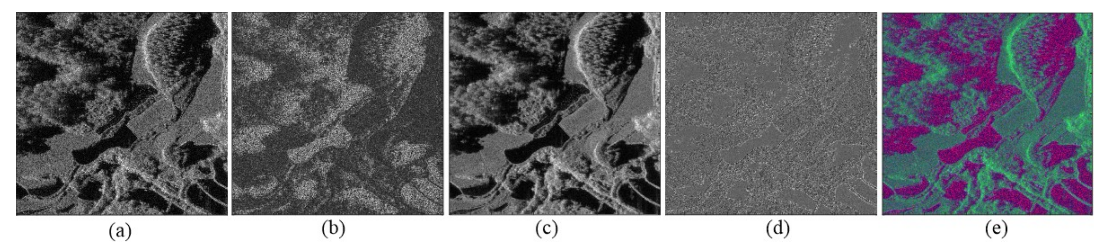
We follow [40,41,42] to heuristically select the features of large gradient dominance, grayscale mean, and correlation as low-level features to reduce the speckle noise, as shown in Figure 3. Figure 3a is the SAR image, and Figure 3b is the lager gradient dominance feature. Figure 3c is the grayscale mean, which reduces the noise in a big extent, and Figure 3d is the correlation. They extract the different texture features for better classification. Since most existing deep neural networks expect input images with three channels [43,44], so we follow this to construct the input with three channels. The three features (as shown in Figure 3b–d)) are concatenated to form a three-channel input, which is shown in Figure 3e.
4.2. The Encoder Network
The Encoder network is composed of ResNet with 101 layers. ResNet is used to perform image classification initially. According to the FCN proposed by Long et al. [23], the network used for classification should be changed to FCN for dense classification, if the Global Average Pooling (GAP), fully connected layer, and Softmax layer in the residual network are removed.
4.2.1. Residual Network
For image classification, there are several excellent networks, such as RefineNet [27], VGG-19 network [45], FCN [23], ResNet [36,46], and DenseNet [35].
In traditional CNN, the network is simply stacked one layer by another, as shown in Figure 4a. We assume that the function of any layer in the network is expressed as , then the output of the th layer can be represented as:
where , , and are the input, output, and the weight of the -th layer.
He et al. [36,46] has observed that the performance of network would not be improved by simply stacking layers, which might even decrease when the number of layers was too deep. Therefore, they have presented Residual network (ResNet), which made CNN break through the limitation of layers depth and achieved better feature representation within deeper layers. The ResNet is stacked by a series of residual units, which is shown in Figure 4b. Instead of calculating the output directly, each residual unit calculates a residual and then adds it to the input :
Using Equation (7) recursively, He et al. [46] has demonstrated the output of the th residual unit as:
The above equation shows that the network has good backpropagation performance. Assuming the Loss function of the network is , the following relation can be obtained according to the backward chain rule [47]:
The update of the weights depends on and . Only the latter depends on the depth of the network, not the former. Meanwhile, there will be no gradient disappearance if their sum is not zero. This is rarely the case, so the gradient can be smoothly transmitted from the upper layers of the network to the lower layers, enabling the training of deeper networks.
4.2.2. The Structure of the Encoder Network
The specific structure of the Encoder network is shown in Table 1. In the matrix of Conv2_x of Table 1, and 64 denote the size and number of the convolutional kernel, and means the number of the residual convolutional unit, which contains three convolutional layers. The 101-layer refers to the number of the weight layers in the network, and the specific calculation method is (3 + 4 + 23 + 3) × 3 + 1 + 1 =101, without the fully connected layer. In Table 1, the initial value of the image for Output size is assumed to be 512 × 512.
4.3. The Decoder Network
The internal structure of Decoder network is shown in Figure 2. It contains two MFEF networks, and each of them includes four Global Convolutional Networks (GCNs), four DecoderLSTM_X (X = 1, 2, 3, 4) modules or four Decoder_X (X = 1, 2, 3, 4) modules, and the Dense connections.
4.3.1. Global Convolutional Network
GCN is composed of two separable convolutions [48], and , which is shown in Figure 5a. GCN can implement dense connections in a region of the input feature map, and its calculations and parameters are only compared with the ordinary convolutional kernel. GCN performs dense connection [28] in the large receptive field in the network, which can improve the accuracy the classification results and has the function of dimension matching.
4.3.2. DecoderLSTM_X Module
The four DecoderLSTM_X (X = 1,2,3,4) modules have the same internal structures with different parameters. This module consists of three parts (as shown in Figure 5b), namely, Residual Convolution Unit (RCU), Multi-Resolution Fusion (MRF), and Improved Chained Residual Pooling (ICRP). In the Decoder Network, the DecoderLSTM_X has multiple inputs, including high-resolution features generated from the Encoder network and low-resolution semantic features output by the DecoderLSTM_Y (Y > X). The feature output by the Encoder network is processed by two RCU units and then fused with low-resolution semantic features. Then the fused features are processed further by the ICRP module to extract new semantic features, which will be tuned by an RCU unit and then they will be output to the higher-resolution decoder module (e.g., DecoderLSTM_X (X = 2, 3, 4)) or processed to generate the score map (DecoderLSTM_1). Where DecoderLSTM_4 has only one input from the feature generated by the Encoder.
(A) Residual Convolution Unit
The Residual Convolution Unit (RCU) consists of the residual convolution unit [27] without the Batch Normalization (BN) layer. The main functionality of RCU is to fine-tune the weight of the pre-trained residual network model, and meanwhile, it can adjust the input features for the following processing. The structure of RCU is shown in Figure 6a, which includes two Relu layers and two 3 × 3 convolutional layers.
(B) Multi-Resolution Fusion
The Multi-Resolution Fusion (MRF) module is shown in Figure 6b, whose functionality is to fuse the features generated by the Encoder and the features output by the Decoder module with higher-level. Assuming H, W, and C are the height, width, and channel number of the input feature map, then their consistency needs to be guaranteed before the fusion of features with different resolutions. First, the channel number C of the input features from the current Encoder and the previous Decoder module is unified by a convolution operation, and if there are dense connected inputs, the dimension matching should be performed through the Global Convolutional Network (GCN). Then, all low-resolution feature maps are upsampled to high-resolution feature map to ensure the uniform of .
(C) Improved Chained Residual Pooling
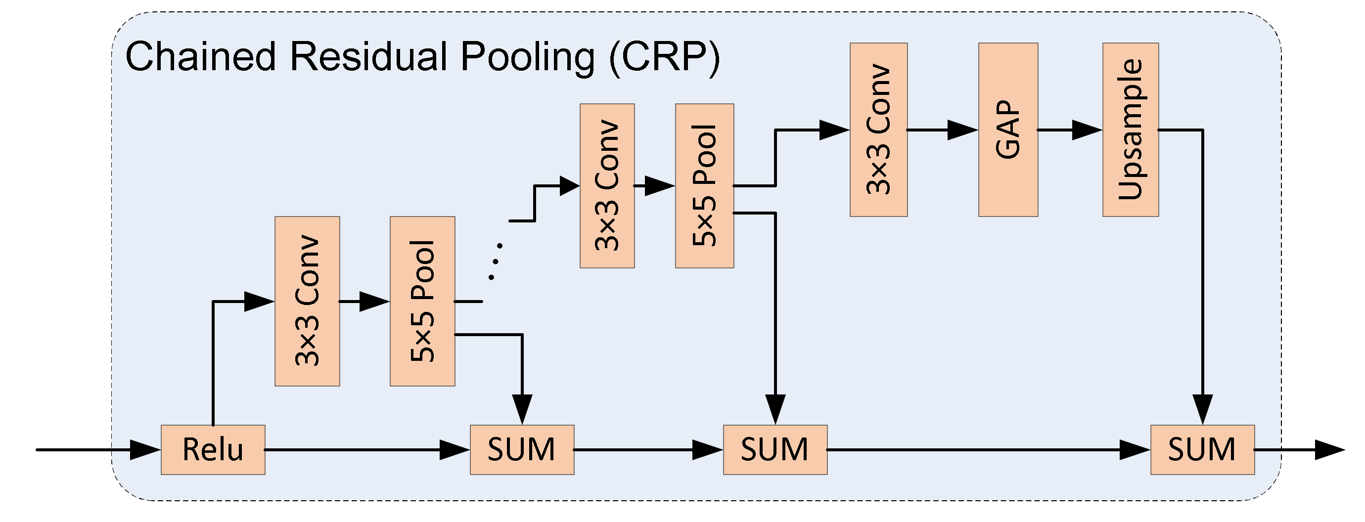
The Chained Residual Pooling (CRP) developed by Lin et al. [27] can be used to extract the contextual information from the background in a large image area, playing an important role in the Decoder module. It is also used in [49], and the only difference of CRP is that CONCAT operation is used to fuse the pooled features instead of SUM used in RefineNet [27]. In this paper, we introduce Convolutional Long Short-Term Memory (ConvLSTM) into the CRP to simultaneously handle spatio-temporal sequences.
• Convolutional Long Short-Term Memory
Long Short-Term Memory (LSTM) [50] is a type of Recurrent Neural Network (RNN) [51]. Its internal memory units could store and process the information across a wide range of time, which help solve the problem of gradient disappearance in RNN. LSTM has been widely used in various fields. Visin et al. [52] has proposed the Renet network for image classification. It is completely built by LSTM, which is a very meaningful attempt though the result is slightly worse than the network built by convolution and pooling. Li et al. [37] has presented LSTM-CF network for image classification. It inserts several LSTM layers into the CNN to extract a broad range of dependence relation among pixels, which gains good classification performance compared to the local receptive field of the convolution network. However, the vector conversion required by LSTM has always incurred considerable spatial structure information loss, since LSTM is based on temporal sequential data, not spatial data. Therefore, Shi et al. [53] has developed the Convolutional LSTM (ConvLSTM) network to solve this problem by introducing a convolutional structure into LSTM, which could simultaneously resolve spatio-temporal sequences.
In addition to introducing convolution operations and higher dimensions of data representation, ConvLSTM has a similar structure to LSTM. The main innovation of LSTM is flexible memory unit, which can change the information in the unit through input gates, output gates, and forgetting gates. The forgetting gate and the input gate separately determine how much information will be discarded from the memory unit and how much information will be input into the unit, and the output gate determines how much information will be output based on the current unit.
Suppose the inputs are , and the memory units are . The status of the hidden layer is , and the input gate, the forgetting gate, and the output gate are , respectively. These variables are all 3-D tensors. The symbol ’’ indicates the convolution operation and ’’ indicates the Hadamard product:
where denotes Sigmoid function, and Wx~ and Wh~ are the 2-D convolutional kernels.
The specific structure of ConvLSTM is shown in Figure 7.
• The Improved Chained Residual Pooling module
The proposed Improved Chained Residual Pooling (ICRP) module is shown in Figure 8, in which ConvLSTM is employed.
ICRP has been improved in three aspects compared with CRP. First, we swap the position of convolution layer and the pooling layer, which are implemented as a 5 × 5 maximum pooling layer follows a 3 × 3 convolution layer; and meanwhile the number of the convolution and pooling modules is increased to four. Second, a Global Average Pooling (GAP) is added to obtain the global information of the feature map. As shown in Figure 8, the biggest advantage of CRP is that it can continuously pool the input feature map, so a 5 × 5 window can be used to obtain a wide range of contextual information. Third, ConvLSTM unit is used to integrate the output features of each pooling module. At present, in the network of CRP, the fusion of feature maps in different pooling stages mostly uses SUM [27] or CONCAT [49]. It can be seen from CRP structure [27] that the features output by the previous pooling module will be utilized by the latter pooling module. The difference between the neighboring features is several times of pooling, so there is a certain temporal and spatial correlation among these features. The spatial operation by simple SUM or CONCAT is not enough to generate semantically distinctive features, so ConvLSTM is introduced to integrate the spatial and temporal information of features. ConvLSTM requires the input features to be 5D tensors (i.e., [samples, time, rows, cols, channels]), but the features in CRP are 4D tensors (i.e., [samples, rows, cols, channels]), so we need to increase their dimensionality. As shown in Figure 8, we perform a dimension expansion to features output by each pooling module, connect four features along the time dimension, and bring the generated features to the ConvLSTM unit for further processing to output a 4D feature. We set time for the four feature maps in CRP, namely, , , , and . we first feed the feature of the moment into ConvLSTM, which will generate a memory state of the current feature with a hidden layer state . When the moment comes, ConvLSTM will decide how much previous information to forget and how much new information to add based on the current input and the state of the previous moment. Using such loops, a new feature will be output according to the live memory state. The ICRP can extract better contextual information than CRP, allowing the network to accommodate higher resolution images, and LSTM could also tackle the problem of gradient disappearance.
4.3.3. Decoder X Module
There are two Decoder Modules used in our Decoder Network. One is the DecoderLSTM_X which is introduced above. Another is the Decoder_X module. The difference between them is that ConvLSTM is not used in Decoder_X module. Instead of using ICRP, we implement Chained Residual Pooling (CRP), which is shown in Figure 9. It consists of series of 3 × 3 Convolution layers and 5 × 5 Pooling layers. Then GAP, upsample, and SUM are used to generate the high-level features, based on traditional CRP [27].
4.3.4. Dense Connection
DenseNet [35] has developed the idea of shorter connections based on the ResNet and has introduced more connections among layers. DenseNet could further mitigate the problem of gradient disappearance and enhance the propagation and reusability of features. Therefore, we follow DenseNet to perform dense connections in the paper. It means that the output of DecoderLSTM_X or Decoder_X (X = 1, 2, 3, 4) is passed to each DecoderLSTM_Y or Decoder_Y, where Y < X (as shown in Figure 2). This allows each DecoderLSTM_X or Decoder_X to use all the previous high-level features, and the features are reused to correct errors from previous Encoder_X (X = 1, 2, 3, 4). The dense connection can effectively fuse features at different resolutions, and the gradient during training can be smoothly transmitted among various decoding modules, alleviating the problem of gradient disappearance.
4.3.5. Score Map Fusion
The score map fusion performs fusion of the two score maps generated by MFEF1 and MFEF2 with different weights and the new splicing method. The specific experiments of MFEF1 and MFEF2 are described in Appendix A. The weights have been determined heuristically, and the new splicing method is introduced as follows.
SAR images used in the paper are all large-scale images, while deep learning requires small-scale input images for training. Therefore, we generally decompose the large-scale image into small-scale images. However, when we cut the original image, we may encounter a situation where a large water body is divided into two or more parts, which undermines the integrity of the target. Although the results can be generated by stitching small images directly, there will be distortion at the edge areas.
To address the problem above, a new splicing method is presented in the paper inspired by Xing and Sieber [54] to reduce or eliminate the errors at the splicing. First, we use a sliding window with the size of 512 × 512 to cut the large-scale image with a stride of 256. It can minimize the probability of object cutting in input images and repeat testing for almost all the areas of the image to reduce the probability of misclassification. Then, the splicing of testing results is performed. In this process, the score map matrixes output by the network are used instead of the classified images. For the overlapping regions of score maps, weighted averaging is employed to reduce splicing errors. By this means, all processed areas are spliced into one whole score map, which is fed to the Softmax layer to generate the classification probability of each position and the index map is finally produced.
5. Experiments and Results
5.1. Study Area
In the experiment, an area of a large-scale SAR image with a size of 4096 × 4608 is tested using the trained model. The SAR image is shown in Figure 10a. In the experiment, we get the large gradient dominance, the grayscale mean feature, the correlation feature, and the fusion feature for the SAR image, which are shown in Figure 10b–e respectively. According to Figure 10e, the water and shadow areas are different from other targets. Figure 10f shows the ground truth of the SAR image.
5.2. Adjustment of the Number of Feature Maps
The most time-consuming part of deep neural work is the training stage, which is significantly influenced by the depth of the network, the number of parameters, and the number of feature maps that need to be calculated. The size of the output of the 101-layer residual network is 256, 512, 1024, and 2048. There are two advantages to do so: one is to reduce the utilization of memory; while the other is to save the training time.
To address problems above, four sets of comparative experiments are carried out using the dataset. The number of the feature maps is set to 1, 1/2, 1/4, and 1/8 of the original RefineNet respectively. Individual results are shown in Table 2. The time in Table 2 refers to the average time to perform one subset training [55], which contains 200 images. We set the batch size to 1 due to the limited memory on the Graphic Processing Unit (GPU), and we employ subsets for better organization in the training. The accuracy is the accuracy of the validation set, and the evaluation criterion used is the Mean Intersection over Union (MIoU) [56,57]. MIoU is the most commonly used evaluation criterion for deep learning-based classification. It calculates the ratio of the intersection and the union between the segmentation results and the labels. The specific calculation formula is as follows:
where is the sum of the pixels belonging to the type both in the label and the classification result, and is the sum of the pixels which are type in the label but type in the classification result. is the number of classes (k = 2 in the paper, which stands for water and shadow). The other targets are marked as the background. Therefore, there are three categories in total.
According to the experiment results, when the numbers of the feature maps input into the Decoder are 64, 64, 64, and 128, the MIoU of the validating set is only reduced by 0.1%, but the training time is nearly half less than the original setting (256, 256, 256, and 512). Therefore, this configuration of feature maps (64, 64, 64, and 128) are used to train the network in the study.
5.3. Setting of Training Parameters and Data Enhancement
During the training of the network, the learning rate and the weight decay are set to and 0.995 respectively. For GCN module between the Encoder module and the Decoder module, the size of the convolution kernel is set to , and is 64, 64, 64, and 128, respectively. In the Multi-Resolution Fusion (MRF) module, the setting of the GCN parameter is the same as before, and is adjusted according to the dimension of the input high-resolution feature from the encoder module. In the ConvLSTM, the size of convolutional kernel is set to 3 × 3, and the stride is set to 1. During the training, some traditional data enhancement operations are also adopted to process the dataset, such as horizontal and vertical mirroring, and random cropping with a window size of 512 × 512.
5.4. Results and Analysis
A total of two sets of comparative experiments have been done to validate the performance of the proposed framework. The first set of experiment is to test the proposed framework with different network configurations, such as Encoder_MFEF2, Encoder_MFEF1, GLGCM_Encoder_MFEF1, GLGCM_Encoder_MFEF1_2, and Lee_Encoder_MFEF1. All these bold ones represent the corresponding frameworks. Encoder_MFEF2 or Encoder_MFEF1 denotes it only uses the framework combining the Encoder network and the MFEF2 network or MFEF1 network in Figure 1 to perform classification for SAR images, which we use to compare their abilities of classification. GLGCM_Encoder_MFEF1 denotes it uses the same framework as Encoder_MFEF1 to perform classification by adding GLGCM features of the SAR image. GLGCM_Encoder_MFEF1_2 uses the same framework as GLGCM_Encoder_MFEF1, but the final classification result is generated by the new splicing method proposed in Section 4.3.5. Lee_Encoder_MFEF1 uses the same framework as Encoder_MFEF1 to perform classification for 5 × 5 Lee-filtered [58] SAR images. The proposed network in the paper (MRDED, as shown in Figure 1) also adopts the new splicing method in Section 4.3.5. While the second set of experiment is mainly to compare the proposed framework with several other existing and main stream deep learning frameworks in SAR images classification, such as FCN-8S [23], the RefineNet [27], Large_Kernel_Matters [28], and ResNet-101_FCN [36].
The classification accuracy (testing accuracy) of the first set of experiment is shown in Table 3. ‘PA’ means pixel accuracy, namely, the percentage of the correctly classified pixels to the total pixels, which is computed by Equation (17). ‘MPA’ denotes Mean Pixel Accuracy, which can be computed by Equation (18):
where denotes the number of pixels that are type but are classified as type , and is the total number of the types.
From Table 3, we can see the proposed framework Encoder_MFEF2 could reach the PA of 0.9101 and MIoU of 0.7651. The proposed framework Encoder_MFEF1 could acquire better PA than Encoder_MFEF2, which indicates the introduced ConvLSTM can improve the classification, but the improvement is not very big. Lee_Encoder_MFEF1 gives the worst classification accuracy of these framework. That may be because the Signal and Noise Ratio (SNR) of the SAR image is very good, the detailed information of the targets is destroyed when using Lee filter again. The PA of GLGCM_Encoder_MFEF1 is 0.41% less accurate than Encoder_MFEF1, but its MPA and MIoU are 0.56% and 0.6% higher respectively. Which proves that GLGCM is good for improving classification accuracy. The PA and MIoU of GLGCM_Encoder_MFEF1_2 are 1.02% and 1.59% higher respectively than GLGCM_Encoder_MFEF1, which proves the effectiveness of the new splicing method. The proposed framework MRDED obtains the best performance, suggesting that MRDED is a powerful framework for water and shadow classification.
To further analyze the classification performance of the proposed framework, the second set of experiment gives a comparison between MRDED and other classification frameworks. The classification results are shown in Figure 11, and the accuracy of the frameworks is shown in Table 4. For simplicity, we use EN_M1, L_En_M1, R-101_FCN, G_En_M1, G_En_M1_2, and L_K_M to represent Encoder_MFEF1, Lee_Encoder_MFEF1, ResNet-101_FCN, GLGCM_Encoder_MFEF1, GLGCM_Encoder_MFEF1_2, and Large_Kernel_Matters respectively.
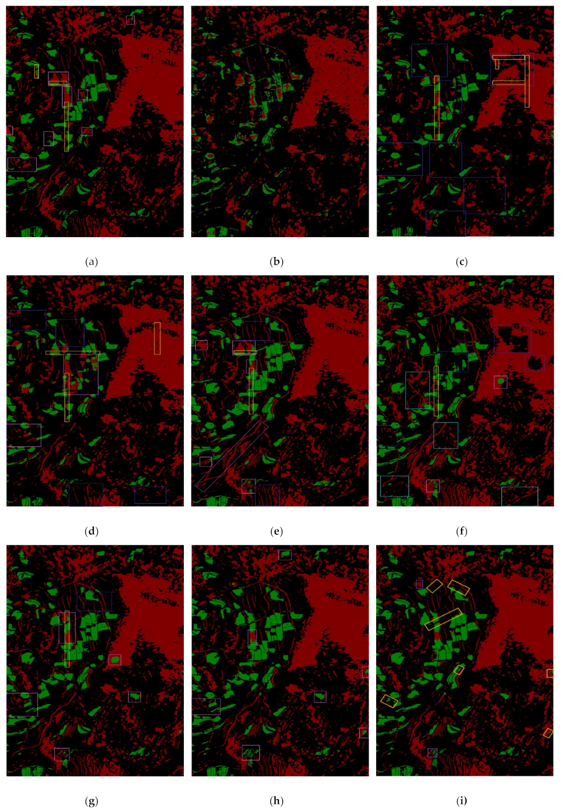
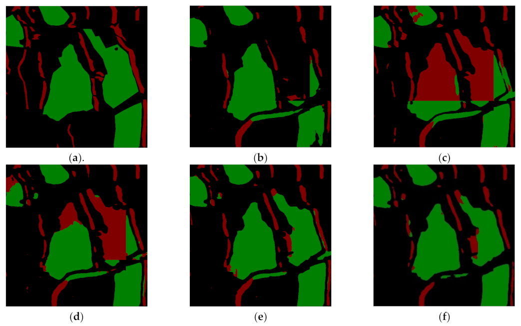
According to Figure 11a, we find there are many misclassified areas compared with the ground truth (as shown in Figure 10f), such as the areas inside the pink rectangles. In these areas, lots of water bodies are misclassified as shadow. Therefore, the classification accuracy for water is lower, only with a PA of 0.6276. The classification accuracy for shadow is higher, with a PA of 0.8829. Therefore, the classification performance of RefineNet for water and shadow from SAR image is not good. In addition, we can see obvious boundary lines at the splicing, which are marked with yellow rectangles. It indicates that it is easy to generate misclassification at the slicing.
Figure 11b–d display the classification result by FCN-8s, ResNet-101_FCN, and Large_Kernel_Matters respectively from the SAR image. In original FCN-8s framework, VGG-19 network is used to extract features, while ResNet-101_FCN, Large_Kernel_Matters, and the frameworks proposed in the paper all use ResNet-101 network. Therefore, for easy and fair comparison of the algorithms, ResNet-101 network is used in ResNet-101_FCN framework instead of VGG-19 network. We find in Figure 11b, there are many missed detection and false detection areas for water and shadow. From Table 4, we could also see the PAs for water and shadow are very low, and the MIoU is only 0.6166. However, while using ResNet-101 network to replace VGG-19 network, the classification accuracy is improved significantly, especially for water extraction, with the improvement from 0.4011 to 0.5769. The corresponding results in Figure 11c also clearly show this. We find that it does not have much improvement in the classification accuracy of the shadow areas, and there are still many missed detection areas (the blue rectangles in Figure 11c). Compared with VGG-19, ResNet-101 could extract more distinguishing features in the experiment. While for Large_Kernel_Matters, as a codec network, it does not directly fuse the multi-layer features extracted by the basic network (VGG-19) but uses the decoding network to process the features generated by the coding network. It achieves much better classification result than FCN-8s and ResNet-101_FCN in shadow, and a less accuracy than ResNet-101_FCN in the tern of water and background, which could be seen in Figure 11d and Table 4. However, there are still some obvious missed areas and misclassified areas. According to the comparable experiment for the extraction of water and shadow using the three frameworks, we find a good coding network can extract more distinctive features, and a good decoding network can further fuse and process features generated by the encoding network for better classification results.
While using the first framework Encoder_MFEF1 proposed in the paper, it achieves much better classification result than all the four previous frameworks (RefineNet, FCN-8s, ResNet-101_FCN, and Large_Kernel_Matters) used in the paper, which is shown in Figure 11e and Table 4. It produces better detailed information and reduces the misclassification between water and shadow. Compared with Figure 11c,d the splicing problem is also solved. Therefore, the introduced ConvLSTM could improve the performance of the framework, and finally increases the classification accuracy. According to Table 4, the PAs of water and shadow are 0.7147 and 0.8955, respectively, and MIoU is 0.7699, which indicates the proposed framework Encoder_MFEF1 is effective in improving classification accuracy for water and shadow from SAR images. Nevertheless, there are still several misclassified areas (the pink rectangles) and missed classified areas (the blue rectangles). For the framework of Lee_Encoder_MFEF1, according to Figure 11f, we find that lots of water and shadow areas are not detected (the blue rectangles), and many false alarm areas exist (the cyan-blue rectangles). The classification accuracies and IoU are all reduced compared with the framework of Encoder_MFEF1 according to Table 4, Which indicates that simply filtering the SAR image and discarding the detailed information of the image would reduce the accuracy of the final classification result.
By integrating the GLGCM features of the SAR image into the framework of Encoder_MFEF1, we get the framework of GLGCM_Encoder_MFEF1, the classification of which is shown in Figure 11g. We find that the classification accuracy of water is better than Encoder_MFEF1 according to Table 4, probably improved by 6%, and the accuracies of shadow and background are slightly lower, but the MPA and MIoU both increases. Which proves the effect of extracting texture features with GLGCM to improve classification accuracy. When the new splicing method (Section 4.3.5) is introduced, we get the framework of GLGCM_Encoder_MFEF1_2, the classification result is shown in Figure 11h. All the classified results of the previous frameworks have the obvious splicing problem, but it is solved in this framework. In Figure 11h, there is almost no splicing problem, and the final classification result is improved too. Though the PA is a little lower than the framework of G_En_M1, but its IoU is higher, and the accuracy of shadow is greatly improved. The final MIoU is increased nearly by 1.6%. However, we find there are still several misclassified areas and the PA of water is only 75.73%.
The classification result of MRDED is shown in Figure 11i. For MRDED, the weights of 0.7 and 0.3 are used for the fusion of the two score maps generated by MFEF2 and MFEF1 respectively. Because we find through numerous experiments that MFEF2 could achieve slightly better classification results for water than MFEF1, though MFEF1 could achieve much better overall classification for the three types of targets. Through many experiments, we select the weight of 0.7 for MFEF2 and the weight of 0.3 for MFEF1. As a result, we find that MRDED achieves better classification results for water and shadow in many orange rectangles areas than GLGCM_Encoder_MFEF1_2, but there are several purple rectangles areas with a slightly worse classification result. The accuracy for water extraction is greatly improved, nearly by 4.4% in PA and 3% in IoU. The accuracy for shadow is reduced by 1.95% in PA, but its IoU is increased by 0.62%. The final MPA and MIoU are improved by 1.09% and 1.3% respectively, which prove that MRDED framework is the best framework in auto-extraction of water and shadow from SAR images.
For more detailed analysis of the classification performance with splicing, Figure 12 shows local enlargements of the classification result generated by different frameworks. We find there are obvious splicing phenomenon, misclassification or missed classification in Figure 12 b–d, because we fuse the classification results by directly splicing. However, when we use the new splicing method (Section 4.3.5), the splicing phenomenon disappears, and misclassification is reduced significantly in Figure 12e, while in Figure 12f, the proposed framework further improves the classification accuracy for water and shadows.
In order to understand the classification performance of various frameworks more intuitively, accuracies for the same type of target with different frameworks have been given in Figure 13 according to Table 4. The abscissa axis represents the nine types of frameworks, and the ordinate axis represents the accuracy of the same type of target. From Figure 13a, for water classification, we find the worst classification performance is the framework of FCN-8s, only with PA and IoU of nearly 0.4, and the best classification effect is the framework of MRDED, with PA of 0.8 and IoU of nearly 0.74. For shadow classification, according to Figure 13b, the frameworks of EN_M1 and G_EN_M1_2 achieve better classification results than the other frameworks, but G_EN_M1_2 has higher IoU than EN_M1 because of the introduction of new splicing method and the GLGCM features. The proposed framework MRDED and the framework of RefineNet achieve slightly lower PA than EN_M1 and G_EN_M1_2, but the MRDED has higher IoU than the other frameworks, which proves it is a more reliable framework for shadow classification. For background classification, according to Figure 13c, FCN-8s and R-101_FCN achieve in PA of over 98%, but their IoUs are very low, which show there are many false alarm areas for background classification. Though the classification accuracy of MRDED is not the highest (only 95%), but its IoU is quite satisfying, which indicates its false alarm areas for background classification are the best. Figure 13d shows the overall accuracy of the three types of targets, including PA, MPA, and MIoU. From which we find, FCN-8s has the worst classification performance, and the proposed framework of MRDED has the best classification results. The final PA, MPA, and MIoU of MRDED could reach 0.9244, 0.8776, and 0.8049, respectively.
In the paper, MRDED, a new framework specifically designed for water and shadow extraction from SAR images has been presented. It has achieved enhanced performance in our experiment. However, there are still several problems that need to be further explored. The first one is the optimization of weights to fuse the two score maps generated by MFEF1 and MFEF2 modules. In the paper, we give the weights of 0.7 for MFEF2 and 0.3 for MFEF1, respectively, following experiments, but how to optimize their values automatically still remains an open challenge, which will be a focus of our future work. The second one is how to further improve the classification performance of the MRDED. Comparing Figure 11i with the ground truth (Figure 10f), we find some water areas and roads are misclassified as shadows; and some shadow areas are classified as background or water. Therefore, we plan to investigate the scattering characteristics of water and shadow in SAR images in the future, to further ameliorate the classification accuracy. Third, the accuracy of water extraction is not very high (80.12%), since we have limited number of water samples in our experiment. This needs to be trained with SAR images covering larger water bodies. The last problem is the boundary of water and shadow extraction. As shown in Figure 12, we find the boundary extraction is not very satisfying with ground-truthing, especially the missing of details. Thus, we will consider other features for detailed boundary representation, especially some segmentation methods to improve the extraction results of water and shadow.
6. Conclusions
In the paper, a new framework, MRDED, has been presented to perform the extraction of water and shadow from large-scale SAR images. It contains three parts, namely, the GLGCM, the Encoder network, and the Decoder network. The GLGCM extracts low-level features from SAR images. The Encoder network is based on the ResNet to extract features with different resolutions. The proposed Decoder network includes two parts, called MFEF and SF, respectively. The MFEF performs the extraction and fusion of the features to generate the score map for classification. In this paper, two MFEF modules are proposed and used to generate separate score maps, which are titled MFEF1 and MFEF2. The only difference between them lies in that ConvLSTM is introduced into MFEF1, which is not utilized in MFEF2. Then, the two score maps are fused with different weights to generate the final score map, which is processed using the Softmax function for the extraction of water and shadow. The proposed framework has integrated CNN, DensNet, ResNet, ConvLSTM, and GCN to achieve enhanced performance in water and shadow extraction from SAR images.
Compared with eight other frameworks in experiments, the presented MRDED framework achieves the best classification results for water and shadow, though there are still some very small misclassified areas. The PA for water, shadows, and background reaches 80.12%, 88%, and 95.16%, and their IoUs are 73.88%, 77.11%, and 90.49%, respectively. The overall accuracy for the three types of targets (water, shadows, and background) are 92.44% in PA, 87.86% in MPA, and 80.49% in MIoU. Therefore, MRDED presents satisfactory extraction performance for water and shadows from SAR images. Following this paper, researchers who are interested in the extraction and classification of SAR images can introduce other networks or modules to replace the existing MRDED components according to the various needs. For example, the GLGCM part could be substituted by other texture extraction algorithms, such as the Gabor transformation. The Decoder part can also be improved by integrating more modules with similar structure to MFEF1 and MFEF2. The performance of MRDED is very reliable even if SAR images were acquired from different sensing platforms (e.g., satellites, airplanes, and UAVs), at different resolutions, and with different geometric attributes. Because MRDED is based on the fusion of multiscale SAR features via advanced deep neural networks. To summarize, MRDED can be widely applied to perform classification of SAR images, in addition to water and shadow.
Author Contributions
L.C. and P.Z. proposed the framework, designed the experiments and produced the results; P.Z. made the SAR dataset; P.Z., L.C., Z.L., J.X., X.X. and Z.Y. contributed to the discussion of the results. L.C. and P.Z. drafted the manuscript. All authors contributed to the study, reviewed and approved the manuscript.
Funding
This work was partly supported by the National Natural Science Foundation (No. 41201468, 41701536, 61701047, 41674040) of China, partly funded by Natural Science Foundation of Hunan Province (No. 2017JJ3322, 2019JJ50639), partly funded by the Foundation of Hunan, Education Committee, under Grants No. 16B004, No.16C0043 and partly funded by China Scholarship Fund.
Acknowledgments
The Milli-meter InSAR dataset used in this study was provided by Beijing Institute of Radio Measurement.
Conflicts of Interest
The authors declare no conflict of interest.
Appendix A
The specific experiments of MFEF1 & MFEF2 are described as follows:
The networks of MFEF1 and MFEF2 are trained and validated respectively, and then the features output from their last layer are weighted during testing. Finally, the features are processed to generate the final extracted results.
Step 1: training stage.
Perform separate training on MFEF1 and MFEF2 and select the models for testing based on the validated results.
Step 2: testing stage.
The image used for testing is cropped into small images using a sliding window of 512 × 512 and a step of 256.
for iteration = 1:num (images) do
where , are the models of the networks of MFEF1 and MFEF2 respectively, and and are the score maps of MFEF1 and MFEF2 respectively. x and F are the input image and the network function respectively.
end for
Step 3: Fusion stage.
- (1)
- Weighting and fusion of the obtained score maps:where and are the weights, and they obey .
- (2)
- Fuse the obtained score maps of the small regions to generate the corresponding score map of the large-scale image.
- (3)
- Input the obtained score map matrix of the large-scale image to the Softmax function to generate the Belief map:b = Softmax(yfuse)
- (4)
- Each pixel of the belief map has a confidence probability belonging to each category, then the category corresponding to the maximum confidence probability is selected as the classified category. Finally, the classification results are fused with colormap to generate the final extracted results.
References
- Skrunes, S.; Brekke, C.; Eltoft, T.; Kudryavtsev, V. Comparing near-coincident C-and X-band SAR acquisitions of marine oil spills. IEEE Trans. Geosci. Remote Sens. 2015, 53, 1958–1975. [Google Scholar] [CrossRef]
- Iervolino, P.; Guida, R.; Iodice, A.; Riccio, D. Flooding water depth estimation with high-resolution SAR. IEEE Trans. Geosci. Remote Sens. 2015, 53, 2295–2307. [Google Scholar] [CrossRef]
- Irwin, K.; Beaulne, D.; Braun, A.; Fotopoulos, G. Fusion of SAR, optical images and airborne LiDAR for surface water detection. Remote Sens. 2017, 9, 890. [Google Scholar] [CrossRef]
- Feng, D.; Wang, T.; Chen, W. Shadow extraction of buildings from high-resolution SAR data via the combination of amplitude reversal and total variation. In Proceedings of the 2015 IEEE 5th Asia-Pacific Conference on Synthetic Aperture Radar (APSAR), Singapore, 1–4 September 2015; pp. 788–791. [Google Scholar]
- Zeng, T.; Gao, Q.; Ding, Z.; Chen, J.; Li, G. Road Network Extraction from Low-Contrast SAR Images. IEEE Geosci. Remote Sens. Lett. 2019, 16, 907–911. [Google Scholar] [CrossRef]
- Kottayil, N.K.; Zimmer, A.; Mukherjee, S.; Sun, X.; Ghuman, P.; Cheng, I. Accurate Pixel-Based Noise Estimation for InSAR Interferograms. In Proceedings of the 2018 IEEE SENSORS, New Delhi, India, 28–31 October 2018; pp. 1–4. [Google Scholar]
- Dubois, C.; Thiele, A.; Hinz, S. Building detection and building parameter retrieval in InSAR phase images. ISPRS J. Photogramm. Remote Sens. 2016, 114, 228–241. [Google Scholar] [CrossRef]
- Du, Y.N.; Feng, G.C.; Li, Z.W.; Zhu, J.J.; Peng, X. Generation of high precision DEM from TerraSAR-X/TanDEM-X. Chin. J. Geophys. 2015, 58, 1634–1644. [Google Scholar]
- Li, Z.; Fielding, E.J.; Cross, P. Integration of InSAR time-series analysis and water-vapor correction for mapping postseismic motion after the 2003 Bam (Iran) earthquake. IEEE Trans. Geosci. Remote Sens. 2009, 47, 3220–3230. [Google Scholar]
- Hinton, G.E.; Salakhutdinov, R.R. Reducing the dimensionality of data with neural networks. Science 2006, 313, 504–507. [Google Scholar] [CrossRef]
- Chen, Y.; Lin, Z.; Zhao, X.; Wang, G.; Gu, Y. Deep learning-based classification of hyperspectral data. IEEE J. Sel. Top. Appl. Earth Obs. Remote Sens. 2014, 7, 2094–2107. [Google Scholar] [CrossRef]
- Kussul, N.; Lavreniuk, M.; Skakun, S.; Shelestov, A. Deep learning classification of land cover and crop types using remote sensing data. IEEE Geosci. Remote Sens. Lett. 2017, 14, 778–782. [Google Scholar] [CrossRef]
- Zou, Q.; Ni, L.; Zhang, T.; Wang, Q. Deep learning-based feature selection for remote sensing scene classification. IEEE Geosci. Remote Sens. Lett. 2015, 12, 2321–2325. [Google Scholar] [CrossRef]
- Jennifer Ranjani, J.; Thiruvengadam, S.J. Fast threshold selection algorithm for segmentation of synthetic aperture radar images. IET Radar Sonar Navig. 2012, 6, 788–795. [Google Scholar] [CrossRef]
- Hou, Y.; Guo, L. A novel SAR image segmentation method based on Markov random filed. J. Electron. Inf. Technol. 2007, 29, 1069–1072. [Google Scholar]
- Hong, S.; Jang, H.; Kim, N.; Sohn, H.G. Water Area Extraction Using RADARSAT SAR Images Combined with Landsat Images and Terrain Information. Sensors 2015, 15, 6652–6667. [Google Scholar] [CrossRef] [PubMed]
- Martinis, S.; Kuenzer, C.; Wendleder, A.; Huth, J.; Twele, A.; Roth, A.; Dech, S. Comparing four operational SAR-based water and flood detection approaches. Int. J. Remote Sens. 2015, 36, 3519–3543. [Google Scholar] [CrossRef]
- Xie, L.; Zhang, H.; Wang, C.; Chen, F. Water-Body types identification in urban areas from radarsat-2 fully polarimetric SAR data. Int. J. Appl. Earth Obs. Geoinf. 2016, 50, 10–25. [Google Scholar] [CrossRef]
- Cellier, F.; Oriot, H.; Nicolas, J.M. Introduction of the mean shift algorithm in SAR images: Application to shadow extraction for building reconstruction. In Proceedings of the 25th EARSeL Symposium, Workshop on 3D Remote Sensing, Porto, Portugal, 10–11 June 2005; pp. 1–8. [Google Scholar]
- Tison, C.; Tupin, F.; Maitre, H. Retrieval of building shapes from shadows in high resolution SAR interferometric images. In Proceedings of the 2004 IEEE International Geoscience and Remote Sensing Symposium, Anchorage, AK, USA, 20–24 September 2004; Volume 3, pp. 1788–1791. [Google Scholar]
- Jahangir, M.; Blacknell, D.; Moate, C.P.; Hill, R.D. Extracting information from shadows in SAR images. In Proceedings of the 2007 International Conference on Machine Vision, Islamabad, Pakistan, 28–29 December 2007; pp. 107–112. [Google Scholar]
- Papson, S.; Narayanan, R. Modeling of target shadows for SAR image classification. In Proceedings of the 35th IEEE Applied Images and Pattern Recognition Workshop, Washington, DC, USA, 11–13 October 2006; p. 3. [Google Scholar]
- Long, J.; Shelhamer, E.; Darrell, T. Fully convolutional networks for semantic segmentation. In Proceedings of the IEEE conference on computer vision and pattern recognition, Boston, MA, USA, 8–10 June 2015; pp. 3431–3440. [Google Scholar]
- Chen, L.C.; Papandreou, G.; Kokkinos, I.; Murphy, K.; Yuille, A.L. Semantic image segmentation with deep convolutional nets and fully connected CRFs. In Proceedings of the International Conference on Learning Representations 2015, San Diego, CA, USA, 7–9 May 2015; pp. 1–14. [Google Scholar]
- Zheng, S.; Jayasumana, S.; Romera-Paredes, B.; Vineet, V.; Su, Z.; Du, D.; Torr, P.H. Conditional random fields as recurrent neural networks. In Proceedings of the IEEE international conference on computer vision, Boston, MA, USA, 8–10 June 2015; pp. 1529–1537. [Google Scholar]
- Chen, L.C.; Papandreou, G.; Kokkinos, I.; Murphy, K.; Yuille, A.L. Deeplab: Semantic image segmentation with deep convolutional nets, atrous convolution, and fully connected CRFs. IEEE Trans. Pattern Anal. Mach. Intell. 2018, 40, 834–848. [Google Scholar] [CrossRef] [PubMed]
- Lin, G.; Milan, A.; Shen, C.; Reid, I. Refinenet: Multi-path refinement networks for high-resolution semantic segmentation. In Proceedings of the IEEE conference on computer vision and pattern recognition, Honolulu, HI, USA, 22–25 July 2017; pp. 1925–1934. [Google Scholar]
- Peng, C.; Zhang, X.; Yu, G.; Luo, G.; Sun, J. Large Kernel Matters--Improve Semantic Segmentation by Global Convolutional Network. In Proceedings of the IEEE conference on computer vision and pattern recognition, Honolulu, HI, USA, 22–25 July 2017; pp. 4353–4361. [Google Scholar]
- Chen, S.; Wang, H.; Xu, F.; Jin, Y.Q. Target classification using the deep convolutional networks for SAR images. IEEE Trans. Geosci. Remote Sens. 2016, 54, 4806–4817. [Google Scholar] [CrossRef]
- Huang, Z.; Pan, Z.; Lei, B. Transfer learning with deep convolutional neural network for SAR target classification with limited labeled data. Remote Sens. 2017, 9, 907. [Google Scholar] [CrossRef]
- Lin, Z.; Ji, K.; Kang, M.; Leng, X.; Zou, H. Deep convolutional highway unit network for sar target classification with limited labeled training data. IEEE Geosci. Remote Sens. Lett. 2017, 14, 1091–1095. [Google Scholar] [CrossRef]
- Geng, J.; Wang, H.; Fan, J.; Ma, X. Deep supervised and contractive neural network for SAR image classification. IEEE Trans. Geosci. Remote Sens. 2017, 55, 2442–2459. [Google Scholar] [CrossRef]
- Zhang, J.; Xing, M.; Sun, G. A water segmentation method from SAR image based on dense Depthwise separable convolution. J. Radars 2019, 19, 2479. [Google Scholar]
- Krizhevsky, A.; Sutskever, I.; Hinton, G.E. Imagenet classification with deep convolutional neural networks. In Proceedings of the Advances in neural information processing systems, Lake Tahoe, NV, USA, 3–6 December 2012; pp. 1097–1105. [Google Scholar]
- Huang, G.; Liu, Z.; Van Der Maaten, L.; Weinberger, K.Q. Densely connected convolutional networks. In Proceedings of the IEEE conference on computer vision and pattern recognition, Honolulu, HI, USA, 22–25 July 2017; pp. 4700–4708. [Google Scholar]
- He, K.; Zhang, X.; Ren, S.; Sun, J. Deep residual learning for image recognition. In Proceedings of the IEEE conference on computer vision and pattern recognition, Las Vegas, NV, USA, 26 June–1 July 2016; pp. 770–778. [Google Scholar]
- Li, Z.; Gan, Y.; Liang, X.; Yu, Y.; Cheng, H.; Lin, L. Lstm-cf: Unifying context modeling and fusion with lstms for rgb-d scene labeling. In Proceedings of the European conference on computer vision, Cham/Amsterdam, The Netherlands, 11–14 October 2016; pp. 630–645. [Google Scholar]
- Hong, J. Gray Level Gradient Cooccurrence Matrix Texture Analysis Method. ACTA Autom. Sin. 1984, 10, 22–25. [Google Scholar]
- Hou, B.; Ren, B.; Ju, G.; Li, H.; Jiao, L.; Zhao, J. SAR image classification via hierarchical sparse representation and multi-size patch features. IEEE Geosci. Remote Sens. Lett. 2016, 13, 33–37. [Google Scholar] [CrossRef]
- Wang, H.; Dong, F. Image features extraction of gas/liquid two-phase flow in horizontal pipeline by GLCM and GLGCM. In Proceedings of the 2009 9th International Conference on Electronic Measurement & Instruments, Beijing, China, 16–19 August 2009; pp. 135–139. [Google Scholar]
- Geng, J.; Fan, J.; Wang, H.; Ma, X.; Li, B.; Chen, F. High-resolution SAR image classification via deep convolutional autoencoders. IEEE Geosci. Remote Sens. Lett. 2015, 12, 2351–2355. [Google Scholar] [CrossRef]
- Chen, L.; Cui, X.; Li, Z.; Yuan, Z.; Xing, J.; Xing, X.; Jia, Z. A New Deep Learning Algorithm for SAR Scene Classification Based on Spatial Statistical Modeling and Features Re-Calibration. Sensors 2019, 19, 2479. [Google Scholar] [CrossRef]
- Garcia-Garcia, A.; Orts-Escolano, S.; Oprea, S.; Villena-Martinez, V.; Garcia-Rodriguez, J. A review on deep learning techniques applied to semantic segmentation. arXiv 2017, arXiv:1704.06857. [Google Scholar]
- Goodfellow, I.; Bengio, Y.; Courville, A. Deep Learning; MIT press: Cambridge, MA, USA, 2016. [Google Scholar]
- Simonyan, K.; Zisserman, A. Very deep convolutional networks for large-scale image recognition. In Proceedings of the International Conference on Learning Representations, San Diego, CA, USA, 7–9 May 2015; pp. 1–14. [Google Scholar]
- He, K.; Zhang, X.; Ren, S.; Sun, J. Identity mappings in deep residual networks. In Proceedings of the European conference on computer vision, Cham/Amsterdam, The Netherlands, 11–14 October 2016; pp. 630–645. [Google Scholar]
- LeCun, Y.; Boser, B.; Denker, J.S.; Henderson, D.; Howard, R.E.; Hubbard, W.; Jackel, L.D. Backpropagation applied to handwritten zip code recognition. Neural Comput. 1989, 1, 541–551. [Google Scholar] [CrossRef]
- Szegedy, C.; Vanhoucke, V.; Ioffe, S.; Shlens, J.; Wojna, Z. Rethinking the inception architecture for computer vision. In Proceedings of the IEEE conference on computer vision and pattern recognition, Las Vegas, NV, USA, 26 June–1 July 2016; pp. 2818–2826. [Google Scholar]
- Bilinski, P.; Prisacariu, V. Dense decoder shortcut connections for single-pass semantic segmentation. In Proceedings of the IEEE Conference on Computer Vision and Pattern Recognition, Salty Lake, UT, USA, 18–22 June 2018; pp. 6596–6605. [Google Scholar]
- Hochreiter, S.; Schmidhuber, J. Long short-term memory. Neural Comput. 1997, 9, 1735–1780. [Google Scholar] [CrossRef]
- Mikolov, T.; Karafiát, M.; Burget, L.; Černocký, J.; Khudanpur, S. Recurrent neural network based language model. In Proceedings of the Eleventh Annual Conference of the International Speech Communication Association, Chiba, Japan, 26–30 September 2010; pp. 1045–1048. [Google Scholar]
- Visin, F.; Kastner, K.; Cho, K.; Matteucci, M.; Courville, A.; Bengio, Y. Renet: A recurrent neural network based alternative to convolutional networks. arXiv 2015, arXiv:1505.00393. [Google Scholar]
- Shi, X.; Chen, Z.; Wang, H.; Yeung, D.Y.; Wong, W.K.; Woo, W.C. Convolutional LSTM network: A machine learning approach for precipitation nowcasting. In Proceedings of the Advances in Neural Information Processing Systems, Montreal, QC, Canada, 7–12 December 2015; pp. 802–810. [Google Scholar]
- Xing, J.; Sieber, R. Sampling based image splitting in large scale distributed computing of earth observation data. In Proceedings of the 2014 IEEE Geoscience and Remote Sensing Symposium, Québec, QC, Canada, 13–18 July 2014; pp. 1409–1412. [Google Scholar]
- Kotsiantis, S.B.; Zaharakis, I.; Pintelas, P. Supervised machine learning: A review of classification techniques. Emerg. Artif. Intell. Appl. Comput. Eng. 2007, 160, 3–24. [Google Scholar]
- Rakhlin, A.; Davydow, A.; Nikolenko, S.I. Land Cover Classification from Satellite Imagery with U-Net and Lovasz-Softmax Loss. In Proceedings of the 2018 IEEE/CVF Conference on Computer Vision and Pattern Recognition Workshops, Salt Lake City, UT, USA, 18–22 June 2018; pp. 262–266. [Google Scholar]
- Cao, R.; Zhu, J.; Tu, W.; Li, Q.; Cao, J.; Liu, B.; Qiu, G. Integrating Aerial and Street View Images for Urban Land Use Classification. Remote Sens. 2018, 10, 1553. [Google Scholar] [CrossRef]
- Yommy, A.S.; Liu, R.; Wu, S. SAR image despeckling using refined Lee filter. In Proceedings of the 2015 7th International Conference on Intelligent Human-Machine Systems and Cybernetics, Hangzhou, China, 26–27 August 2015; pp. 260–265. [Google Scholar]
Figure 1.
(a) the large-scale SAR image. (b) The corresponding ground truth of the SAR image. ‘S’, ‘W’, and ‘B’ denote ‘Shadow’, ‘Water’, and ‘Background’ respectively.
Figure 1.
(a) the large-scale SAR image. (b) The corresponding ground truth of the SAR image. ‘S’, ‘W’, and ‘B’ denote ‘Shadow’, ‘Water’, and ‘Background’ respectively.

Figure 2.
The overall architecture of the proposed network. MRDED denotes Multi-resolution Dense Encoder and Decoder framework, which contains GLGCM feature, Encoder network and Decoder network. The input is SAR images, and the output is the final extracted results of water and shadow.
Figure 2.
The overall architecture of the proposed network. MRDED denotes Multi-resolution Dense Encoder and Decoder framework, which contains GLGCM feature, Encoder network and Decoder network. The input is SAR images, and the output is the final extracted results of water and shadow.

Figure 3.
(a) SAR image. (b) Large gradient dominance. (c) Grayscale mean. (d) Coherence. (e) Fusion feature of (b), (c) and (d).
Figure 3.
(a) SAR image. (b) Large gradient dominance. (c) Grayscale mean. (d) Coherence. (e) Fusion feature of (b), (c) and (d).

Figure 4.
(a) The traditional convolutional neural network. (b) Residual unit.

Figure 5.
(a) The GCN network. (b) The network of DecoderLSTM_X.

Figure 6.
(a) the structure of RCU. (b) the structure of MRF.

Figure 7.
The structure of ConvLSTM. The new memory and output will be generated by updating the internal memory according to the current input and the previous output .
Figure 7.
The structure of ConvLSTM. The new memory and output will be generated by updating the internal memory according to the current input and the previous output .

Figure 8.
The structure of Improved Chained Residual Pooling (ICRP). 4D and 5D denote 4-dimensional tensor and 5-dimensional tensor respectively.
Figure 8.
The structure of Improved Chained Residual Pooling (ICRP). 4D and 5D denote 4-dimensional tensor and 5-dimensional tensor respectively.

Figure 9.
The structure of the Chained Residual Pooling (CRP).

Figure 10.
The SAR image, features and ground truth. (a) SAR image. (b) Large gradient dominant feature. (c) The grayscale mean feature. (d) The correlation feature. (e) The fusion feature of (a), (b) and (c). (f) The ground truth, the red color, green color, and black color denote shadow, water, and background respectively.

Figure 11.
The extracted results for water and shadow from the SAR image. (a) The extracted results by RefineNet. (b) the extracted results by FCN-8s. (c) The extracted results by ResNet-101_FCN. (d) The extracted results by Large_Kernel_Matters. (e) The extracted result by Encoder_MFEF1. (f) The extracted result by Lee_Encoder_MFEF1. (g) The extracted result by GLGCM_Encoder_MFEF1. (h) The extracted result by GLGCM_Encoder_MFEF1_2. (i) The extracted result by MRDED. (j) The fusion map of SAR image and (i). (k) The visualization result of the results by MRDED. (l) Colors description for the classification results from (a) to (j).


Figure 12.
Local segmentation results of different networks proposed in this paper. (a) The ground truth. (b) Lee_Encoder_MFEF1 result. (c) Encoder_MFEF1 result. (d) GLGCM_Encoder_MFEF1 result. (e) GLGCM_Encoder_MFEF1_2 result. (f) MRDED result. The red color and green color denote shadow and water respectively.

Figure 13.
The accuracies for different types of targets with different frameworks. (a) The classification accuracy for water with different frameworks. (b) The classification accuracy for shadow with different frameworks. (c) The classification accuracy for background with different frameworks. (d) The overall accuracy for the three targets.


Table 1.
The network configuration of the Encoder part.
| Layer Name | Output Size | 101-Layer |
|---|---|---|
| Conv1 | 256 × 256 | 7×7, 64, stride 2 |
| 3×3 max pool, stride 2 | ||
| Conv2_x | 128 × 128 | |
| Conv3_x | 64 × 64 | |
| Conv4_x | 32 × 32 | |
| Conv5_x | 16 × 16 |
Table 2.
The experiments for the adjustment of the number of feature maps.
| Number of the Feature Maps | MIoU | Time (s) |
|---|---|---|
| 256, 256, 256, 512 | 74.2 | 101 |
| 128, 128, 128, 256 | 74.2 | 70 |
| 64, 64, 64, 128 | 74.1 | 56 |
| 32, 32, 32, 64 | 73.8 | 52 |
Table 3.
The classification accuracy of the first set of experiment.
| Framework | PA | MPA | MIoU |
|---|---|---|---|
| Encoder_MFEF2 | 0.9101 | 0.8500 | 0.7651 |
| Encoder_MFEF1 | 0.9145 | 0.8561 | 0.7699 |
| Lee_Encoder_MFEF1 | 0.8885 | 0.7949 | 0.7208 |
| GLGCM_Encoder_MFEF1 | 0.9104 | 0.8617 | 0.7759 |
| GLGCM_Encoder_MFEF1_2 | 0.9206 | 0.8667 | 0.7918 |
| MRDED | 0.9244 | 0.8776 | 0.8049 |
Table 4.
The classification accuracy of the different frameworks.
| Framework | Water | Shadow | Background | PA | MPA | MIoU | |||
|---|---|---|---|---|---|---|---|---|---|
| PA | IoU | PA | IoU | PA | IoU | ||||
| RefineNet | 0.6276 | 0.6058 | 0.8829 | 0.7538 | 0.9536 | 0.8932 | 0.9098 | 0.8214 | 0.7509 |
| FCN-8s | 0.4011 | 0.3786 | 0.6764 | 0.6176 | 0.9814 | 0.8537 | 0.8695 | 0.6863 | 0.6166 |
| R-101_FCN | 0.5790 | 0.5576 | 0.6773 | 0.6389 | 0.9871 | 0.8557 | 0.8785 | 0.7478 | 0.6841 |
| L_K_M | 0.5548 | 0.5381 | 0.8083 | 0.7068 | 0.9719 | 0.8871 | 0.8981 | 0.7783 | 0.7107 |
| En_M1 | 0.7147 | 0.6636 | 0.8955 | 0.7481 | 0.9399 | 0.8979 | 0.9145 | 0.8500 | 0.7699 |
| L_En_M1 | 0.6968 | 0.6463 | 0.8646 | 0.6837 | 0.9082 | 0.8466 | 0.8803 | 0.8232 | 0.7255 |
| G_En_M1 | 0.7748 | 0.6956 | 0.8684 | 0.7414 | 0.9419 | 0.8908 | 0.9104 | 0.8617 | 0.7759 |
| G_En_M1_2 | 0.7573 | 0.7089 | 0.8995 | 0.7649 | 0.9433 | 0.9015 | 0.9206 | 0.8667 | 0.7918 |
| MRDED | 0.8012 | 0.7388 | 0.8800 | 0.7711 | 0.9516 | 09049 | 0.9244 | 0.8776 | 0.8049 |
© 2019 by the authors. Licensee MDPI, Basel, Switzerland. This article is an open access article distributed under the terms and conditions of the Creative Commons Attribution (CC BY) license (http://creativecommons.org/licenses/by/4.0/).
Share and Cite
MDPI and ACS Style
Zhang, P.; Chen, L.; Li, Z.; Xing, J.; Xing, X.; Yuan, Z. Automatic Extraction of Water and Shadow from SAR Images Based on a Multi-Resolution Dense Encoder and Decoder Network. Sensors 2019, 19, 3576. https://doi.org/10.3390/s19163576
AMA Style
Zhang P, Chen L, Li Z, Xing J, Xing X, Yuan Z. Automatic Extraction of Water and Shadow from SAR Images Based on a Multi-Resolution Dense Encoder and Decoder Network. Sensors. 2019; 19(16):3576. https://doi.org/10.3390/s19163576
Chicago/Turabian StyleZhang, Peng, Lifu Chen, Zhenhong Li, Jin Xing, Xuemin Xing, and Zhihui Yuan. 2019. "Automatic Extraction of Water and Shadow from SAR Images Based on a Multi-Resolution Dense Encoder and Decoder Network" Sensors 19, no. 16: 3576. https://doi.org/10.3390/s19163576
Note that from the first issue of 2016, this journal uses article numbers instead of page numbers. See further details here.