1. Introduction
The performance of the Global Navigation Satellite System (GNSS) positioning depends on the accuracies of satellite orbit and clock products [
1,
2]. Thanks to the great effort of the International GNSS Service, for example, the Multi-GNSS Experiment project, several types of precise orbit and clock products for GNSS satellites including GPS (Global Positioning System), GLONASS, Galileo, BeiDou and more are provided in routine base with different latencies and accuracies to meet various positioning demands [
3,
4,
5,
6,
7,
8]. Among these products, the ultra-rapid product is generated for possible real-time applications by predicting orbits and clocks over the next 24 h. However, the precision of the predicted clocks cannot satisfy the requirement of real-time precise point positioning (RTPPP) although the orbit uncertainty of about 5–10 cm can be neglected [
9]. With the growth of GNSS high precision applications, there are already a number of RTPPP providers, such as GFZ (German Research Centre for Geosciences) and Wuhan University. Unfortunately, not all users can use the correction information due to either cost of the service or the user location is not within the coverage area of the service. Therefore, to improve the accuracy of predicted satellite clocks, especially over short-term, is of considerable interest to make RTPPP reliable in the abovementioned circumstances [
10,
11].
Generally, clock prediction is firstly required for generating clock information for broadcast ephemeris. It is an indispensable GNSS function in order to provide standard positioning service and the prediction time could be several hours to a few days varying from system to system. The positioning performance depends heavily on the accuracy of the predicted clocks. Usually, a low-order polynomial model is employed, and the accuracy is about 0.53 ns and 0.64 ns for example for GPS and BeiDou satellite navigation system (BDS), respectively [
12]. Higher accuracy is quite challenging for the prediction process, as the intrinsic physical characteristic of clocks is very complex and unstable also due to varying space environments [
12,
13,
14]. As a result of these factors, usually clock offsets, including clock bias, frequency bias, and drift, contain strong non-linear and stochastic features which make the short-term precise modeling and prediction rather difficult [
13,
15]. Despite such difficulties, numerous studies were carried out, and several models were established for clock prediction, e.g., quadratic polynomial (QP) model, spectrum analysis (SA) model, Kalman filter (KF) and neural network (NN) model [
16,
17].
The widely used prediction models include first and second order polynomial models, for example, and the predicted clock in GPS broadcast ephemeris [
18,
19] are well studied and discussed [
20]. However, it is certificated that the clock error of the quadratic polynomial model is accumulated rapidly with the predicted time increased [
16,
21]. Such a result was expected because the stochastic variations contained by satellite clock accumulated over time [
20]. To improve the QP model, studies obtained four main periodic variances for GPS satellites based on the fast Fourier transform (FFT) method and analyzed the relationship between its amplitude and orbit period [
22]. They show the incorporation of fixed-period harmonics, especially for the GPS satellite clocks, provides a very accurate predicting model. Even though the SA model with periodic terms included is an improvement to quadratic polynomial model, it is pointed out that the periodic function has to be determined reasonably by a rather long clock time series [
14,
17]. Meanwhile, Epstein et al. achieve an accuracy of 8 to 9 ns by predicting GPS clocks over six hours with a KF approach, but the estimation is not reliable due to occurring frequency jumps [
23]. Moreover, artificial neural networks are used by scientists to predict clock offset [
12,
16,
24,
25], e.g., WNN (wavelet neural network) and BPNN (back propagation neural network), which has the ability to estimate non-linear time series by sample training. However, the topology structure of the WNN is hard to set up, while the BPNN needs an iterative procedure to determine the appropriate weights which is considerably time-consuming.
While most of the abovementioned achievements focus on GPS clock, BDS clock attracts more and more attention. There are also three types of real-time clock products for BDS satellites, namely broadcast ephemeris clock products with the accuracy of about 6 ns, ultra-rapid products about 2–6 ns and real-time estimated corrections updated every 5–10 s [
12,
26]. After comparison of these products, it can be concluded that the ultra-rapid product plays an important role in decimeter-level real-time positioning services, which is made available by some analysis centers [
12]. However, evident nonlinear system errors, i.e., periodic signals, are detected in ultra-rapid clock product [
12,
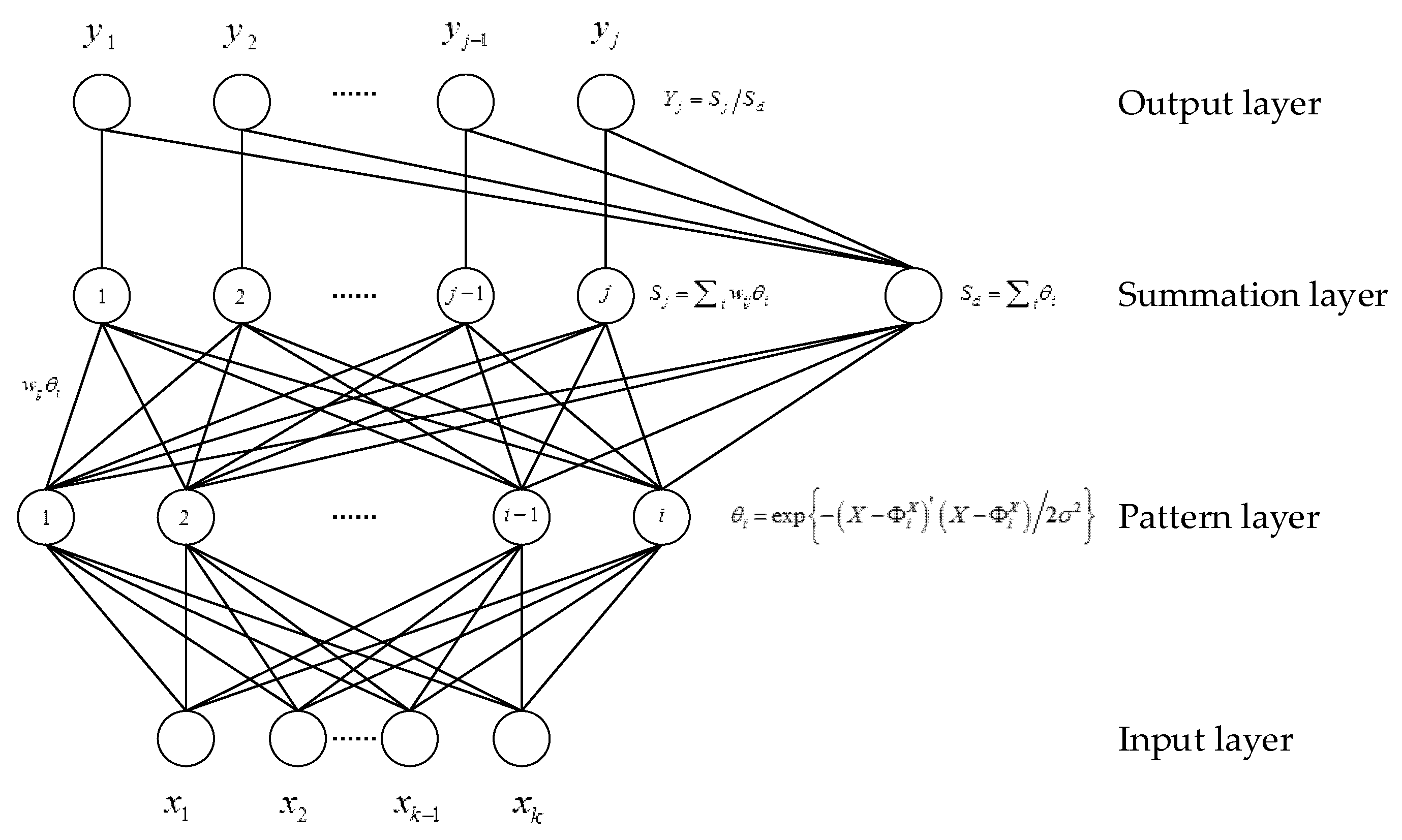
25]. To meet the requirement of highly precise applications, such as early warning and hydrographic surveying, an improved model is required to enhance its prediction. Regarding the benefit from artificial intelligence, GRNN (generalized regression neural network) is a generation of radial basis function networks and probabilistic neural networks proposed by Specht [
27] and has a strong ability of generalization for non-linear and stochastic clocks. In this paper, an improved model based on the SA model and GRNN is developed to deal with BDS-2 satellite clock prediction.
In the following sections, the related typical models for BDS-2 satellite clock prediction are summarized in
Section 2, including the quadratic polynomial model, spectrum analysis model and GRNN. Then, an improved model for BDS-2 satellite clock prediction is proposed, and satellite- specific optimal parameters are determined by experiments in
Section 3. After preprocessing of clock offsets, clock accuracy, static and kinematic precise point positioning (PPP) are validated and analyzed in
Section 4. Finally,
Section 5 concludes with a discussion.
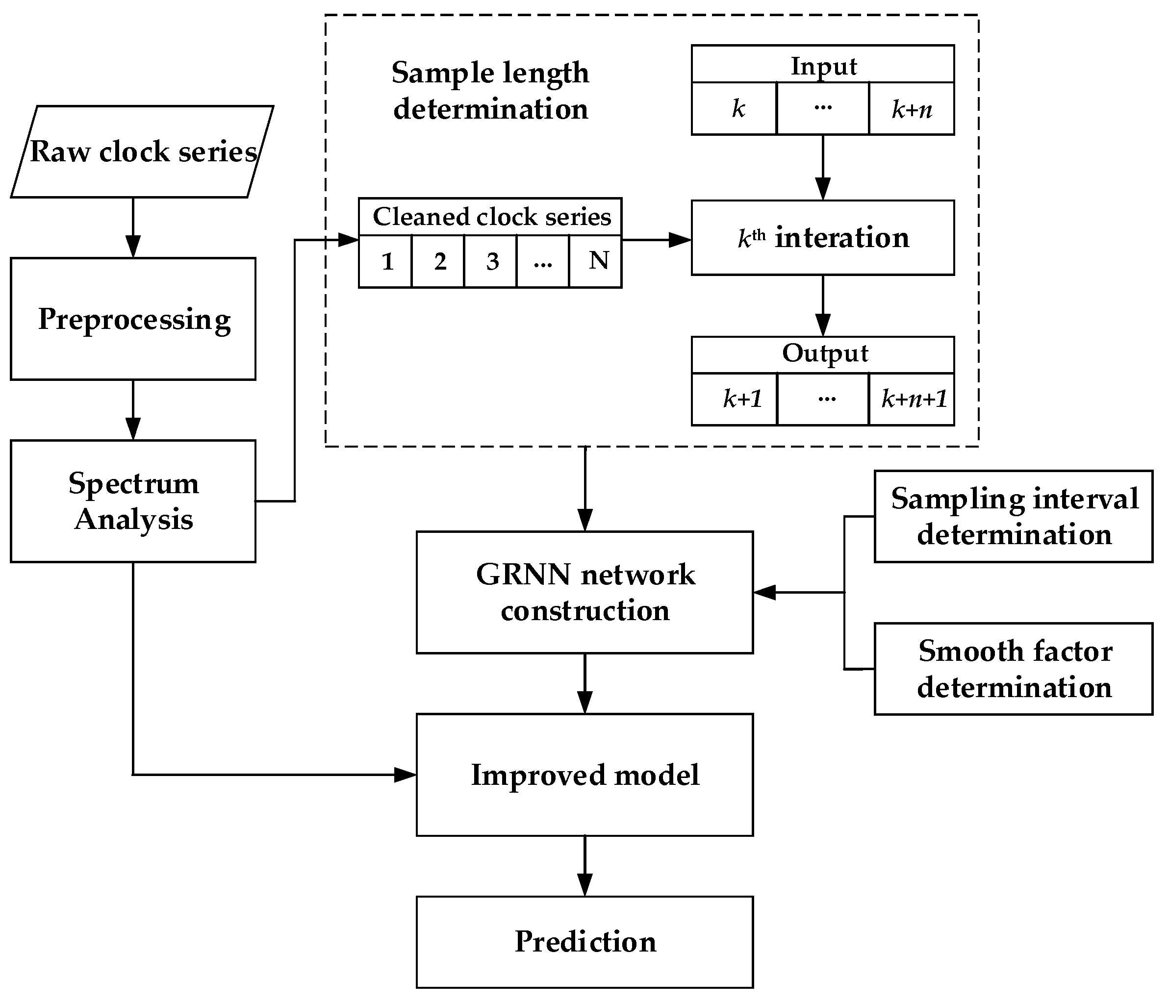
3. Realization of the Improved Model
3.1. Preprocessing for Satellite Clock Offset
The estimated clocks of ultra-rapid products of BDS-2 which are made available by several GNSS analysis centers, for example GFZ, are used as input in data processing. However, the raw clock time series may conceal abnormal data, such as gross errors and blunders, which should be detected before performing clock prediction. The epoch-differenced clocks are calculated in which outliers can be shown more apparently and then the outliers are detected using the median absolute deviation (MAD), which is a robust but simple method [
30]. In addition, the principle not to delete outliers more than 5% of total data is followed here, which avoids losing too much useful information [
25]. Now, this preprocessing method is applied for each BDS-2 satellite using ultra-rapid products of GFZ with 5 min sample interval. Considering satellite clock stability is inversely proportional to its operation time, the newest launched satellites C02, C13, and C14, belong to GEO (Geostationary Earth Orbit), IGSO (Geosynchronous Satellite Orbit), and MEO (Medium Earth Orbit), respectively, are selected as examples to show the effectiveness of the MAD method in
Figure 3.
3.2. Determination of Periodic Terms
Huang indicates that significant periodic characteristics are found in BDS-2 satellite clock residuals after quadratic polynomial fitting and periodic terms vary from satellite to satellite due to different geometric configurations [
12]. In order to find out the potential periods for each BDS-2 satellite clock, FFT is applied to analyze the clock residuals after quadratic polynomial fitting using more than 100 days data from day 001 to day 105 in 2018. The relationships between amplitude and frequency are identified for GEOs, IGSOs, and MEOs, respectively in
Figure 4, and the outstanding periods of each BDS-2 satellite clock are given in
Table 1. Results show 24 h and 12 h are two significant periodic terms for most of GEOs and IGSOs with different amplitudes. As for MEOs, a 12 h harmonic with a smaller amplitude than for GEOs and IGSOs is noticeable. In general, the most noticeable periods of BDS-2 satellite clocks are related to their corresponding orbit periods. Interestingly enough, a special periodic term of about 1.3 h has been detected with a pronounced amplitude for the C11 satellite, and it is different from the normal period of the MEO orbital geometric configuration. This obvious period will have a large impact on prediction accuracy and must be considered. This noticeable period may be caused by the hardware of the atomic clock itself. Additionally, due to the uneven distribution of ground tracking stations and the relatively stable geometry between the GEO satellites and stations, the amount of data of C04 is less than other satellites, which is probably the reason that the residual noise level is large, and it leads to a saw-tooth pattern when doing FFT.
3.3. Impact of the Length of Input Data
The performance of the GRNN network differs in different sample datasets. Meanwhile, to build a suitable GRNN network, a sample dataset is required to be divided into input data and output data in an appropriate way. In this experiment, the remaining clock residues after the removal of trend and periodic terms are used, including all fourteen BDS-2 satellites. In the GRNN network construction phase, the length of input data successively increases from 1 h to 9 h to investigate how the length of input data affects the GRNN network performance. As an example, the length of input data is 5 h, in the first iteration, the GRNN network is constructed based on data of 1–5 h as input and with data 2–6 h as output. By analogy, in the second iteration, the GRNN network is optimized based on data of 2–6 h as input and with data 3–7 h as output. After completion of the (N-5)-th iteration (assuming there are N hour data), the GRNN network is employed for prediction.
Now, we can judge which sample length is the best for each BDS-2 satellite, including 5 GEOs, 6 IGSOs, and 3 MEOs, by checking the agreement of true (GFZ precise clock products) and prediction with different length of input data.
Figure 5 gives clock difference results for each satellite type, and they are on the sub-nanosecond level when the prediction time is less than 1 h, no matter the length of input data raises from 1 h to 9 h. The clock differences for all fourteen BDS-2 satellites increase along with prediction time increasing, but are still within ±2 ns for most satellites, when the prediction time is not more than 3 h.
Figure 5 also shows when a short length of input data is employed, i.e., 1–2 h, the characteristics of the satellite clock cannot be fitted properly. On the other hand, when the length of input data is up to 8–9 h, the clock differences are not the smallest, since too much perturbation information is introduced. After numerous experiments, when the prediction time is less than 3 h, the recommended length of input data is 3 h for most satellites as the best compromise between prediction accuracy and computational complexity. Additionally, it should be noted that the clock differences for all satellite clocks start from zero since the fitting ability of the GRNN is extremely strong and the training set and the test set are continuous.
3.4. Impact of the Sampling Interval of Input Data
Sampling interval reflects the intensive extent of input data, and it is another key parameter in a GRNN network. If the sampling interval is very small, a larger quantity of data joins in the GRNN network construction, and usually, it will lead to better predictions. However, the computation complexity increases dramatically with the number of neurons raising rapidly. With increasing sampling interval, sparse data may cause loss of short-term characteristics and decreasing the prediction accuracy. Therefore, sampling interval selection is worth to investigate for a better balance.
In this experiment, the K-fold cross method is employed to investigate how the sampling interval affects the prediction accuracy, and therefore, the sampling interval of input data is set up to 30 s, 60 s, 120 s, 180 s, 240 s, and 300 s, respectively. The clock differences between true and prediction for two satellites of each type are presented in
Figure 6. Overall, the sampling interval, less than 300 s, has little effect on the prediction accuracy. Additionally, the clock differences increase along with prediction time increasing but are still within ±1 ns for all fourteen BDS-2 satellites. In order to reduce the computing load, 300 s is choosing as the sampling interval in accordance with IGS 5 min clock products.
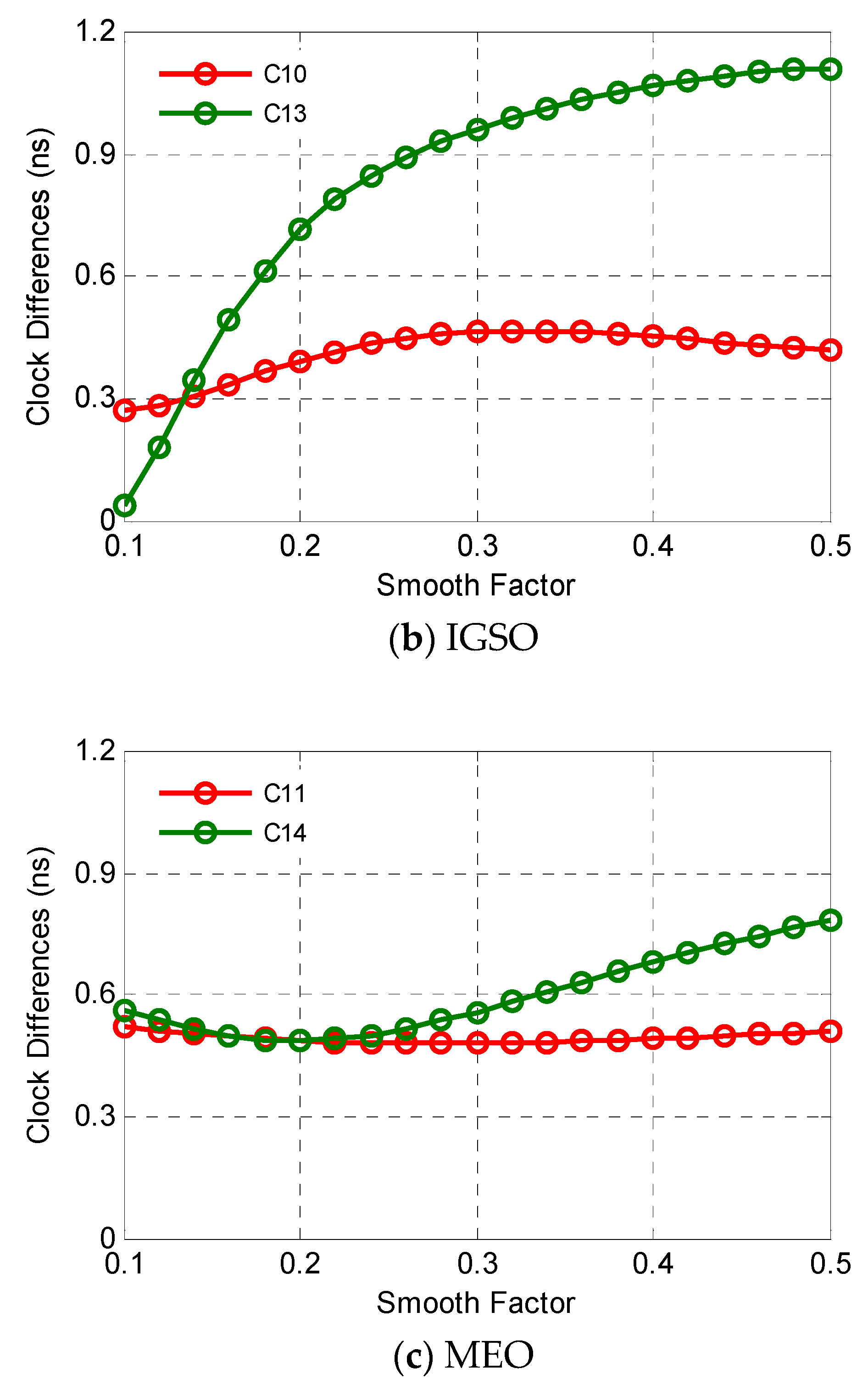
3.5. Determination of the Smooth Factor
Unlike a back propagation neural network, connection weights of a GRNN network are determined when the sample dataset is given. The smooth factor is the only adjustable parameter in a GRNN network, and it is well known that the smooth factor controls the influence sphere of input data, which significantly affects the prediction accuracy. With increasing the value of the smooth factor, the prediction curve is much smoother and neglects details. When the smooth factor is smaller, the approaching performance is better, but at the expense of computing time and the problem of over-fitting. Hence, the smooth factor for a GRNN network is required to carefully determinate.
Since there is no a priori information, the smooth factor is determined by a search method in a special region. A series of values from 0.10 to 0.50 with steps of 0.02 is employed to check the prediction performance.
Figure 7 indicates that the smooth factor should be satellite-specific determined, and the final results are given in
Table 2. Taking C14 as an example, the smooth factor increases from 0.10 to 0.50, the clock differences between true and prediction firstly decrease and then increase with an optimal value of 0.20.
5. Conclusions
Driven by requirements of real-time GNSS precise positioning, short-term precise clock predictions are improved for BDS-2 satellites for possible applications where real-time clock corrections are not available. An improved model combing spectrum analysis and GRNN is proposed. Further, the periodic terms and GRNN related parameters including length and sampling interval of input data, as well as a smooth factor are optimized satellite by satellite to consider satellite-specific characteristics for all the fourteen BDS-2 satellites. For example, there exist some special periods, e.g., 1.3 h for C11, beyond our understanding that periodic terms are related to the orbit period. This noticeable period may be caused by the hardware of the atomic clock itself.
The improved model with satellite-specific parameters is validated by comparing the predicted clocks of existing models and the improved model with precisely estimated ones. The clock accuracy of the improved model is generally better than that of the QP, SA, and GRNN model. The overall accuracy of predicted clocks is better than ±1 ns within 3 h, which is significantly enhanced with respect to the ultra-rapid products and the accuracy is good enough for several real-time precise applications.
The clock prediction is further evaluated by applying them to precise point positioning in both static and kinematic mode for eight IGS MGEX stations in the Asia-Pacific region. The position accuracies using predicted clocks obtained from QP, SA, GRNN models and the improved model are compared and their convergence times are also analyzed as well. In the static PPP, the improved model is validated to be effective, and helps to achieve more than 30.0% improvements on average for each component, which enables some stations to obtain sub-decimeter positioning accuracy. In the kinematic PPP, the improved model performs much better than the others in terms of both convergence time and position accuracy. The convergence time can be shortened from 1–2 h to 0.5–1 h, while the position accuracy is enhanced by 15.4%, 21.6%, and 19.3% on average in east, north and up component, respectively.
Additionally, compared to the polynomial model, the improved model needs extra processing time in the GRNN network construction phase. Supposing that N is the number of the whole data, n is the number of the input data in an iteration that is small enough to be ignored when compared with N, and L is the number of iterations. Therefore, the computational complexity of GRNN is O(NL). However, the GRNN network construction is not a real-time task. Hence, the computing time of the improved model is almost at the same level as for the polynomial model in the clock prediction process.
Furthermore, how to determine the smoothing factor value is a key issue. Generally, the Artificial Intelligence Community recommends the determination method of the smooth factor as the search method, which is an empirical method. A feasible way is determining the value of the smooth factor based on the relationship between the smooth factor and the clock quality determined by the Allan variance. However, it is a challenging topic to build function mapping between the smooth factor and the clock quality, and it is also an interesting topic, which will be investigated in our future work.


